Spatio-Temporal Response of Vegetation Indices to Rainfall and Temperature in A Semiarid Region

Abstract

In this research, vegetation indices (VIs) were analyzed as indicators of the spatio-temporal variation of vegetation in a semi-arid region. For a better understanding of this dynamic, interactions between vegetation and climate should be studied more widely. To this end, the following methodology was proposed: (1) acquire the NDVI, EVI, SAVI, MSAVI, and NDMI by classification of vegetation and land cover categories in a monthly period from 2014 to 2018; (2) perform a geostatistical analysis of rainfall and temperature; and (3) assess the application of ordinary and uncertainty least squares linear regression models to experimental data from the response of vegetation indices to climatic variables through the BiDASys (bivariate data analysis system) program. The proposed methodology was tested in a semi-arid region of Zacatecas, Mexico. It was found that besides the high values in the indices that indicate good health, the climatic variables that have an impact on the study area should be considered given the close relationship with the vegetation. A better correlation of the NDMI and EVI with rainfall and temperature was found, and similarly, the relationship between VIs and climatic factors showed a general time lag effect. This methodology can be considered in management and conservation plans of natural ecosystems, in the context of climate change and sustainable development policies.

1. Introduction

To evaluate the effect of temperature and rainfall on vegetation, it is necessary to understand the temporal and spatial dynamics of the vegetation. Furthermore, land use patterns play a very important role in the evaluation of environmental processes for the sustainable management of natural resources and ecosystems conservation [1]. It has been stated that monitoring vegetation dynamics and land cover changes is fundamental for modeling climatic and hydrological scenarios [2,3].

In this sense, the development of remote sensing (RS) has simplified the generation of new methods based on the analysis of satellite images and the use of geographic information systems (GIS). Remote sensing, is information acquisition from a distance, where satellite data are used to infer topography, vegetation cover, system productivity, and other landscape attributes. Remote sensing instruments accumulate the electromagnetic energy reflected by the sun or reflected energy emitted by some device, such as a radar. This information is detected and collected in different ranges of wavelengths (bands), there is a spectral resolution (number of bands and range of band wavelength width) associated to each sensor, and at the same time, a spatial resolution that indicates the area of minimum ground it represents (cell or grid) [4,5]. Remote sensing and geographic information system (GIS) exploratory techniques are appropriate tools for supporting effective management of the vegetation and other natural resources [6].

In particular, Earth observation satellite systems, such as LANDSAT 8, offer multi-temporal images that are widely used, for example, in the study of land use such as agriculture, forest resources, geology, mapping, water quality, pollution, and vegetation [7]. Vegetation is one natural element that responds to the characteristics of the environment to which it belongs [8], that is why vegetation indices (VIs) have been correlated with other climatic variables, such as, temperature and precipitation, and other variables of the immediate environment, such as geomorphology, altitude, and mountainous systems [9,10].

Furthermore, VIs allow us to evaluate the conditions of ecosystems [11]. Some of these indices use the reflectance from vegetation. Some of the most common indices are the normalized difference vegetation index (NDVI), the enhanced vegetation index (EVI), the soil adjusted vegetation index (SAVI), the modified soil adjusted vegetation index (MSAVI), and the normalized difference moisture index (NDMI). These indices are under the same constraints as the source Landsat surface reflectance products, and are based on the measurement of radiation intensity of certain bands of the electromagnetic spectrum that vegetation emits or reflects, and an estimate of the quantity, quality and development of the vegetation [12,13,14].

Besides, arid and semiarid ecosystems comprise at least one-third of the Earth’s surface, they are characterized by low erratic rainfall between 250–500 mm y⁻¹, with different associations of vegetative cover generally short-grass or scrub vegetation [15,16]. In Mexico, arid and semiarid ecosystems cover more than 50% of its surface; however, they are little studied areas [17]. In recent decades, the impact of human activities has become one of the main transforming agents that contribute to degradation of the ecosystems as one of the major environmental problems after water scarcity in arid areas [2]. Also, there are natural events such as floods or droughts that cause alterations in vegetation cover. The VIs are a valuable parameters that simplifies the understanding of ecosystems facilitating their sustainable management related to water resources [18]. The vegetation in dryland ecosystems is of great importance in supporting global biodiversity, carbon sequestration and the majority of the world’s livestock [19], here the growth of vegetation is controlled by infrequent, discrete, and largely unpredictable water inputs [20]. In this sense, spectral vegetation indices have a long history of use by remote sensing scientists [21], although NDVI is one of the most used, there are other indices that have improved the spectral response of a surface and attenuate other factors such as soil, lighting conditions and atmosphere that can be explored.

Other studies have compared VIs based on several criteria [22]. Piedallu et al. [23], monitored the impact of climate change on vegetation covers, Shao et al. [24] related historical vegetation cover to aridity patterns in the greater desert region of northern China, Birtwistle et al. [25], used an alternative way to map the spatial and temporal variation of precipitation inputs along ephemeral stream channels using NDVI derived from Landsat Thematic Mapper imagery, and Abel et al. [26], monitored of changes in dryland ecosystem functioning. Mugiraneza et al. [27], considered a spatio-temporal evolution of urbanization patterns, using multi-temporal Landsat data and to assess the associated environmental impact using landscape metrics and ecosystem services.

Dutta et al. [28], evaluated of the efficiency of remote sensing and GIS techniques for monitoring the spatio-temporal extent of agricultural drought. Xue and Su [29], performed a review of developments and applications of significant remote sensing vegetation indices.

Studies where the correlations between the NDVI and the climatic variables of precipitation and temperature are compared are widely used; however, it is necessary to include other indices like the NDMI, EVI, SAVI, among others, as effective indicators in the response analysis of the vegetation indices in semiarid areas.

The objective of the study was to evaluate the responses of the VIs to spatio-temporal dynamics of temperature and rainfall for a semi-arid region characterized by having vegetation with greater resilience to climate changes. To evaluate this response, RS, GIS and geostatistical tools were used. The NDVI, EVI, SAVI, MSAVI and NDMI were acquired monthly from 2014 to 2018. The time series record for temperature and precipitation was obtained from 25 weather stations placed in the study area. UWRL regression model was used to assess the correlation between the VIs and the climatic variables.

2. Materials and Methods

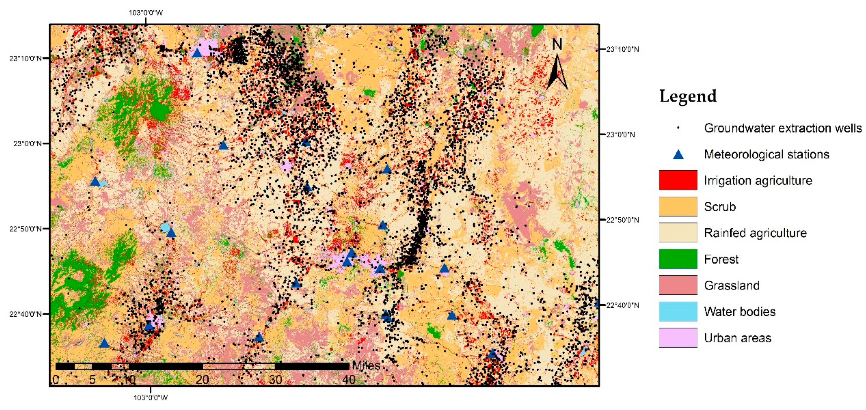
2.1. Study Area (SA)

The study area corresponds to the state of Zacatecas, Mexico, with an area of 11141.56 km². It is considered semiarid with an estimated average monthly temperature for the study area of 16.5 °C and average monthly rainfall of 47.45 mm (period 2014-2018) (Figure 1). The study area is well described by Anuard et al. 2019 [30]. In the study area, the maximum rainfall occurs in the summer. The rainy season extends from May to October, with July, August, and September being the months with the highest rainfall. The dry season begins in November, the month in which the rain is very similar to that of April. The driest months are usually February and March. In December and January there is a slight increase in precipitation due to the cold waves and western circulation. The warm season is from May to September in most of the study area. The warmest months are May and June. October and April are transition months, as the cold season is from November to March, with the coldest being December and January.

The current land cover is explained in

Table 1. Land cover classification in the study area.

Classification	Dominant Species	Description
Irrigation agriculture	Allium sativum	Garlic and onion are potential species for irrigation agriculture in the region.
	Avena sativa
	Allium cepa
Rainfed agriculture	Capsicum annum	Corn and beans are potential species for temporary agriculture in the region [31].
	Phaselous vulgaris
	Zea mays
Forest	Pinus spp.	This ecosystem is dominated by tall trees, mainly pines and oaks accompanied by other species that develop in mountainous areas of cold to temperate climate.
	Cupressus sp.
	Juniperus sp.
	Quercus sp.
Grassland	B. gracilis	They are distributed in semi-arid and cool weather areas. The average annual temperatures range between 12 and 20 °C, with average annual rainfall between 300 and 600 mm. They are found on the slopes of hills and the bottom of valleys with moderately deep, fertile soils and moderately rich in organic matter. In areas with decline and without sufficient protection they erode easily. It corresponds to communities where grasses predominate. The grasslands are medium height (20–70 cm)
	B. scorpioides
	Aristida adscensionis
	Eragrotis mexicana
	E. puchellum
	Leptochola dubia
	Lycurus phleoides
Scrub	Larrea tridentata	It is characterized by having a dry climate with little rainfall (equal to or less than 700 mm per year) in which shrubs of height less than 4 m predominate. In Zacatecas, four scrub subtypes are recognized according to the species that are more common or dominant, microphyllous, rosetophyllus, crasicaule, and spiny [32,33].
	Agave spp.
	Yucca spp.
	Opuntia spp.
	Stenocereus spp.
	Myrtullocactus sp.
	Acacia farneciana
	Prosopis laevigata
	Mimosa spp.

.

2.2. Image Classification and Accuracy Assessment

The Landsat 8 image classification was created using a maximum likelihood classification (MLC), commonly used for thematic mapping with satellite multispectral imagery [34]. The samples were created by selecting about 80% of the sample class data for the satellite image. Seven thematic classes were selected to represent the land cover; the classes were forest, irrigation agriculture, rainfed agriculture, scrub, urban area, water bodies and grassland.

The supervised classification in ArcGIS 10.2.2 allowed to classify the raster by means of each pixel of a cell, for the seven classes, one works with training samples to obtain a final classification of the image. For the irrigation agriculture the classification was made by analyzing the irrigation calendars in order to choose the month that allowed us to differentiate the irrigation and rainfed agriculture areas. April was chosen and different Landsat 8 images of this month were analyzed over the years of study (2014–2018), resulting in the integration of a single classification, which is presented in this study. In addition, the location of the groundwater extraction wells was considered, as sampling points to irrigation agriculture. As well, the other classes were categorized by the type of vegetation and ecoregions, according to the terrestrial ecosystems in Mexico, from the outlook of National Commission for the Knowledge and Use of Biodiversity (CONABIO) [35].

An accuracy assessment was performed to evaluate the performance of the classification algorithm. It was conducted by creating confusion matrices between the land cover maps and the test data, calculating assessment parameters, such as overall classification accuracy (OCA), producer’s accuracy (PA), user’s accuracy (UA), and overall kappa coefficient (OKC). The OKC is a measure of overall statistical agreement of an error matrix, which takes non-diagonal elements into account [36]. The Kappa coefficient is calculated from Equation (1) [37]:

$$kappa=\frac{N{{\displaystyle \sum }}_{i=l}^{K}xil-{{\displaystyle \sum }}_{i=l}^{K\left(1\right)}\left(xi+\ast x+i\right)}{N^2-{{\displaystyle \sum }}_{i=l}^K(xi+\ast x+i)}$$

(1)

where N is the total number of samples, ${\displaystyle \sum }_{i=l}^{K}xil$ is the total correct samples for all classified phenomena, and ${\displaystyle \sum }_{i=l}^K\left(xi+\ast x+i\right)$ is the total product determined by multiplying the total number of samples and the number of correct samples per phenomenon.

2.3. Satellite Imagery

The Landsat 8 images were processed. Landsat 8 and the operational land imager (OLI) provide seasonal coverage of the global landmass at a spatial resolution of 30 meters (visible, NIR, SWIR), 100 meters (thermal), and 15 meters (panchromatic) [38]. These images used the Worldwide Reference System (WRS), a global notation system for Landsat data. It enables a user to inquire about satellite imagery over any portion of the world by specifying a nominal scene center designated by path and row numbers.

The WRS has been proven valuable for the cataloging, referencing, and day-to-day use of imagery transmitted from the Landsat sensors. The Landsat path/row (29/44) covered the study area; one scene per month from 2014 to 2018 was acquired, and the images were processed to remove clouds and were re-projected into the Universal Transverse Mercator (UTM), Datum WGS 84; zone13N.

The Landsat 8 OLI image was obtained from USGS Earth Explorer [39] as a Level-1 Surface Reflectance product. The reflectance calculation was performed in the ArcGis 10.2.2 software. A top of atmosphere (TOA) planetary reflectance value with correction by solar angle (Equation (2) and (3)) [40,41] was applied.

$$\mathsf{\rho }\mathsf{\lambda }{}^{\prime }=\mathrm{M}\mathsf{\rho }\ast \mathrm{Qcal}+\mathrm{A}\mathsf{\rho }$$

(2)

where $\mathsf{\rho }\mathsf{\lambda }{}^{\prime }$= TOA planetary reflectance, without correction for solar angle, $\mathrm{M}\mathsf{\rho }$ = band-specific multiplicative rescaling factor from the metadata, $\mathrm{A}\mathsf{\rho }$= band-specific additive rescaling factor from the metadata, and $\mathrm{Qcal}$= quantized and calibrated standard product pixel values.

The TOA reflectance with a correction for the sun angle is shown by Equation (3).

$$\mathsf{\rho }\mathsf{\lambda }=\frac{\mathsf{\rho }\mathsf{\lambda }{}^{\prime }}{\cos \left({\theta }_{SZ}\right)}=\frac{\mathsf{\rho }\mathsf{\lambda }{}^{\prime }}{\sin \left({\theta }_{SE}\right)}$$

(3)

where $\mathsf{\rho }\mathsf{\lambda }$ = TOA planetary reflectance, ${\theta }_{SE}$ = local sun elevation angle, ${\theta }_{SZ}$= local solar zenith angle, and ${\theta }_{SZ}$= 90° − ${\theta }_{SE}$.

2.4. Vegetation Indices (VIs)

The most used VI is the NDVI, a quotient that represents the functional characteristics of the active plant that contrasts the reflectance of the near infrared and red bands [42] (Equation (4)):

$$NDVI=\frac{NIR-R}{NIR+R}$$

(4)

where NIR corresponds to the near infrared band, and R corresponds to the red band. By definition, the NDVI values vary between +1 and −1 with higher values for dense vegetation and very low (or negative) values for snow, water and clouds [43,44].

The EVI is similar to the NDVI and can be used to quantify vegetation greenness. The EVI corrects for some atmospheric conditions and canopy background noise and is more sensitive in areas with dense vegetation. It incorporates an “L” value to adjust for canopy background, “C” values as coefficients for atmospheric resistance and values from the blue band. These enhancements allow for index calculation as a ratio between the R and NIR values while reducing the background noise, atmospheric noise, and saturation in most cases (Equation (5)).

$$EVI=G\frac{\rho NIR-\rho RED}{\rho NIR+C_1\ast \rho RED-C_{2\ast }\rho BLUE+L}$$

(5)

Here, $\rho$ is the atmospherically corrected or partially atmospherically corrected surface reflectance, L is the canopy background adjustment that addresses nonlinear and different NIR and R radiant transfer through the canopy, and C₁ and C₂ are the coefficients of the aerosol resistance term, which uses the blue band to correct for aerosol influences in the red band. The coefficients adopted in the EVI algorithm are L = 1, C₁ = 6, C₂ = 7.5 and G (gain factor) = 2.5 [45].

The SAVI is used to correct NDVI for the influence of soil brightness in areas where vegetative cover is low. Landsat surface reflectance-derived SAVI is calculated as a ratio between the R and NIR values with a soil brightness correction factor (L) defined as 0.5 to accommodate most land cover types (Equation (6)).

$$SAVI=\frac{NIR-R}{NIR+R+L}\ast \left(1+L\right)$$

(6)

The MSAVI minimizes the effect of bare soil on the SAVI. MSAVI is calculated as a ratio between the R and NIR values with an inductive L function applied to maximize reduction of soil effects on the vegetation signal (Equation (7)) [46].

$$MSAVI=2\ast \rho NIR+1-\frac{\sqrt{{(2\rho NIR+1)}^2-8\left(\rho NIR-\rho RED\right)}}{2}$$

(7)

The NDMI is used to determine vegetation water content. It is calculated as a ratio between the NIR and SWIR values in the traditional fashion (Equation (8)):

$$NDMI=\frac{NIR-SWIR 1}{NIR+SWIR 1}$$

(8)

where SWIR is the short-wave infrared [14].

2.5. Climatological Time Series

A geostatistical analysis was carried out with the climatological database of the National Water Commission (CONAGUA), provided by the State Hydrometeorology Department. The average monthly rainfall and temperature values for the period of 2014–2018 from 25 weather stations were analyzed. Inverse distance weighting (IDW) was used. This is a widely used interpolation method, both for small and large datasets. The unknown value is calculated based on all known points and is inversely proportional to their distances [47].

2.6. Bivariate Analysis

The BiDASys (Bivariate Data Analysis System) program was used for the application of ordinary and uncertainty least squares linear regression models to experimental data from the response of vegetation indices to climatic variables. It applies recursive discordancy tests to both models (studentized residuals) for the detection of discordant outliers. The uncertainty weighted linear regression (UWLR) were applied. The UWLR should is considered as a better alternative because the use of uncertainty has a probability connotation with a strict confidence level of 99%, which was used in the present study. The regressions were acquired correlating the average monthly values of temperature and rainfall (obtained by IDW) and the average values of each VI classification [48,49].

3. Results

3.1. Image Classification

According to the classification, the current soil use corresponds to 792.82 km² of forest (7.12%), 915.40 km² of irrigation agriculture (8.22%), 4487.39 km² of rainfed agriculture (40.28%), 3207.27 km² of scrub (28.79%), 1430.74 km² of grassland, 28.13 km² of water bodies (0.25%), and 279.82 km² of urban area (2.51%) (Figure 2).

3.2. Accuracy Assessment

The classification accuracy is presented in

Table 2. Classification accuracy for land cover map.

Land Cover	Producer’s Accuracy (%)	User’s Accuracy (%)
Irrigation Agriculture	40/40 = 100.00%	40/48 = 83.33%
Scrub	133/152 = 87.50%	133/142 = 93.66%
Rainfed Agriculture	177/185 = 95.68%	177/193 = 91.71%
Forest	26/36 = 72.22%	26/27 = 96.30%
Grassland	65/66 = 98.48%	65/68 = 95.59%
Water	20/20 = 100.00%	20/20 = 100.00%
Urban Area	20/20 = 100.00%	20/21 = 95.24%

; the accuracy of the satellite image classifications was approximately 92.68%. The Kappa coefficient was 90.33%.

To evaluate the results of land cover, the confusion matrix for the land cover map was created (

Table 3. Confusion matrix for land cover map.

Confusion Matrix for Land Cover Map
Reference Data (Number of points)
Land Cover	Irrigation Agriculture	Scrub	Rainfed Agriculture	Forest	Grassland	Water	Urban Area	Ground Truth
Irrigation Agriculture	40	1	3	4	0	0	0	48
Scrub	0	133	4	5	0	0	0	142
Rainfed Agriculture	0	15	177	0	1	0	0	193
Forest	0	1	0	26	0	0	0	27
Grassland	0	2	1	0	65	0	0	68
Water	0	0	0	0	0	20	0	20
Urban Area	0	0	0	1	0	0	20	21
Total	40	152	185	36	66	20	20	519

). In the table, the column of ground truth represents the accuracy along the matrix and the total numbers of points for each classification. An accuracy of 83.33% was found for the classification of irrigation agriculture, 93.66% for scrub, 91.71% for rainfed agriculture, 96.30% for forest, 95.59% for grassland, 100% for water bodies, and 95.24% for the urban area.

These results indicate minor fluctuations in the classification.

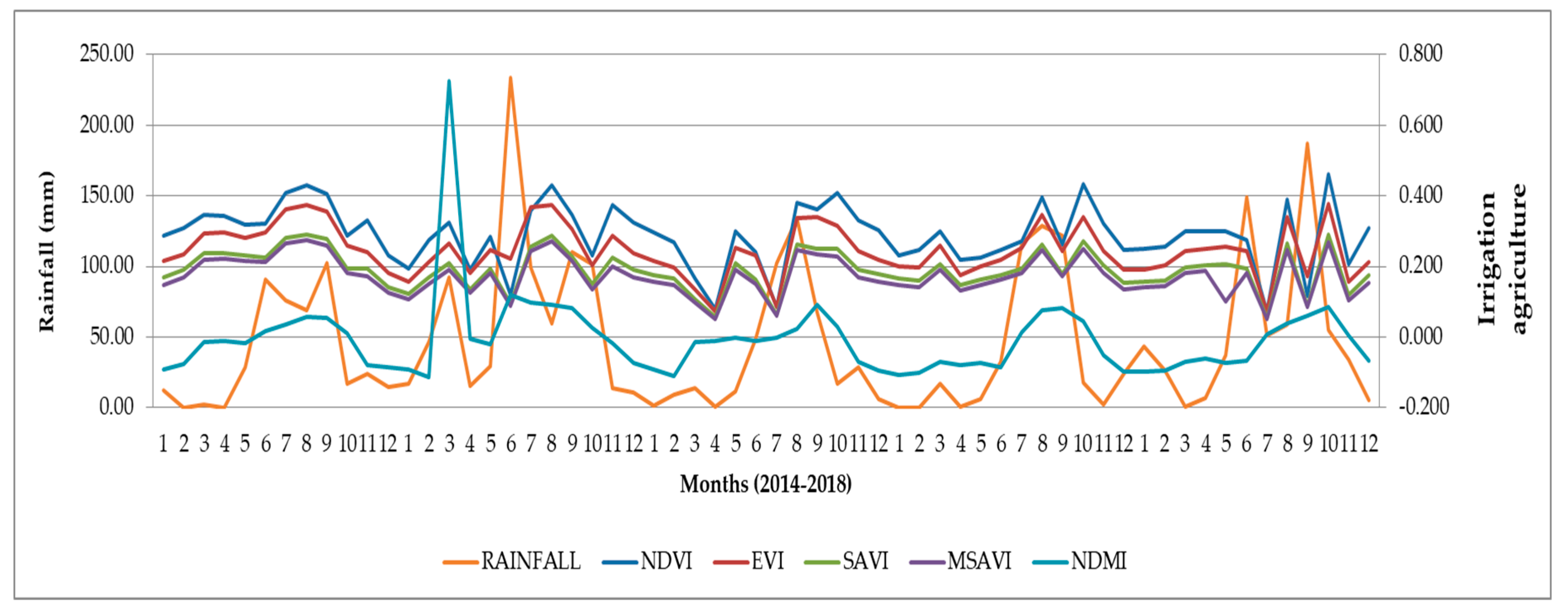
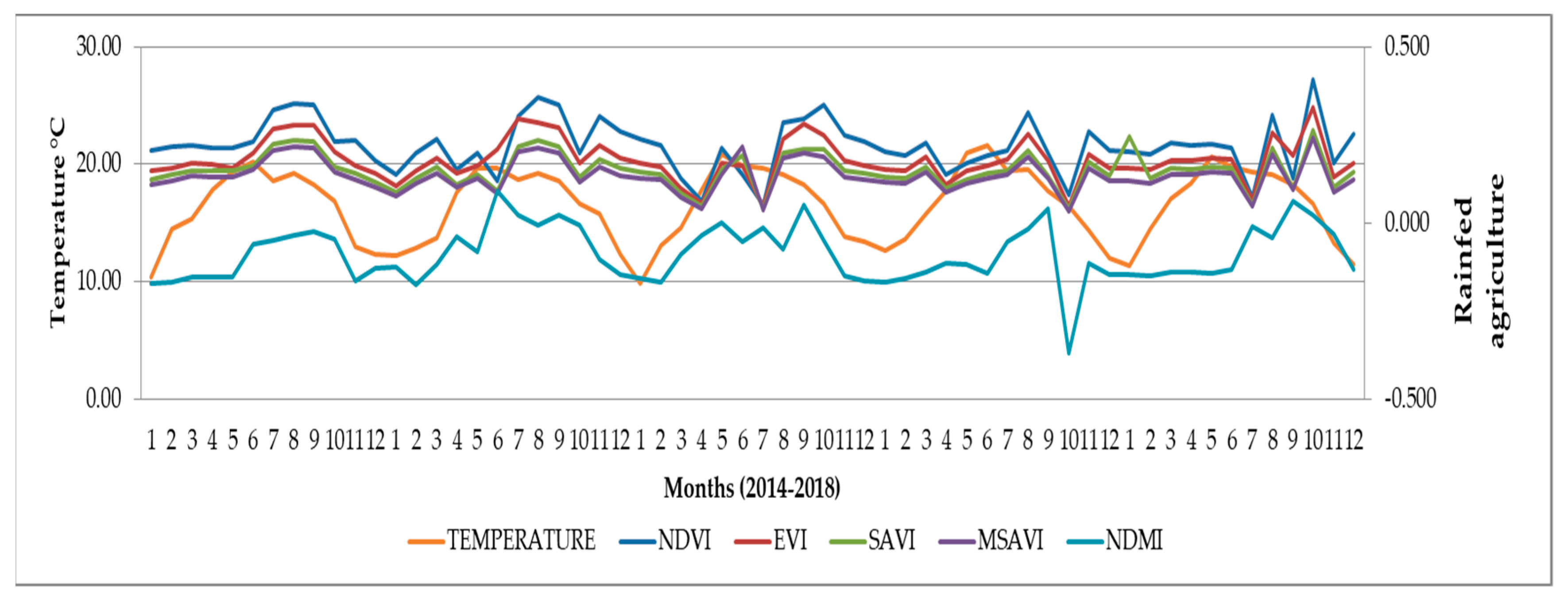
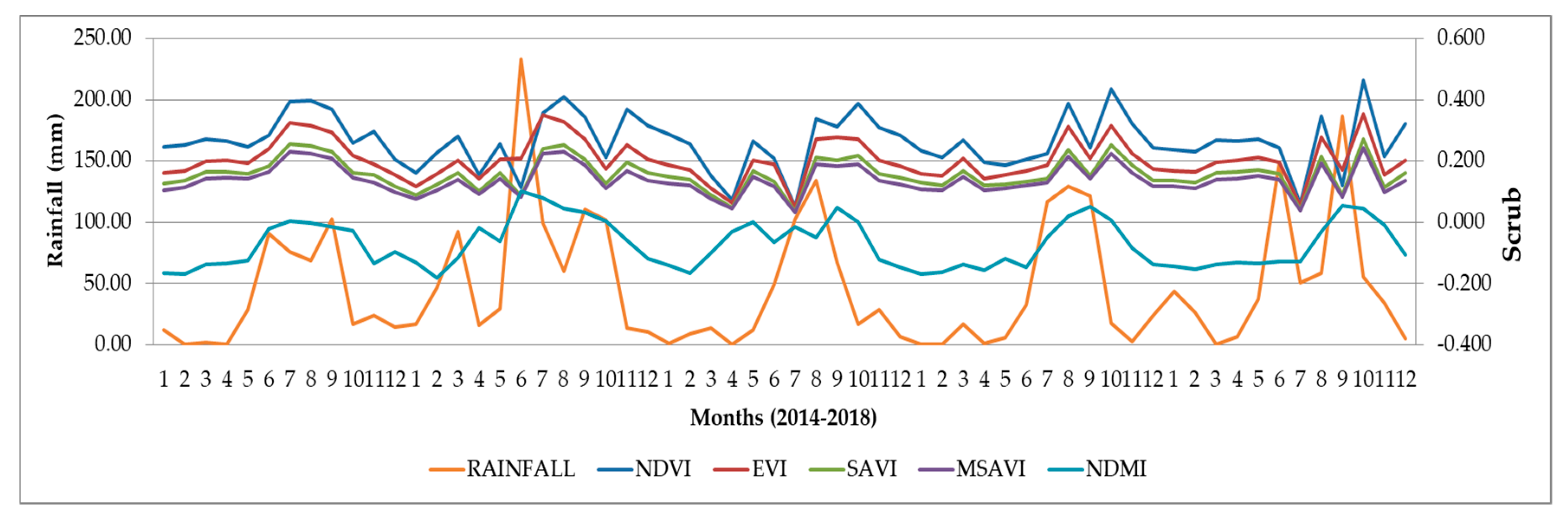
3.3. Spatio-Temporal Patterns of VIs and Climatic Variables

The spatio-temporal changes in the VIs were highly seasonal; the evolution of the VIs in the monthly time series showd a parallel dependence on the behavior of vegetation and changes in rainfall and temperature. In 2014 and 2015, the highest VI values were observed in summer and autumn, the lowest in spring and winter. In 2016, the highest values were in autumn and winter, and the lowest were in summer and spring. In 2017, the highest values were in autumn and summer, and the lowest were in winter and spring, and in 2018, the highest were in autumn and spring, and the lowest were in winter and summer.

In some cases, where the rain exceeds 200 mm (for example, June 2015), values close to 0 were obtained, reflected low values in the VIs. The NDMI values indicated a low canopy cover and dry cover (Figure 3, Figure 4, Figure 5, Figure 6, Figure 7, Figure 8, Figure 9, Figure 10, Figure 11 and Figure 12).

In the rainfed agriculture classification, the VIs showed a very low cover, with values decreasing from the NDVI, EVI, SAVI to MSAVI, in this order of values nearest to zero. The NDMI showed a mid-to-low cover with high water stress (Figure 9 and Figure 10).

In the scrub classification, the VIs showed a very low cover with values decreasing from the NDVI, EVI, SAVI to MSAVI, in this order of values nearest to zero. The NDMI showed a low cover with low water stress (Figure 11 and Figure 12).

There was a positive correlation between the indices and climatic variables which implies that, as the vegetation begins to turn green, the temperature and precipitation also increase and vice versa. The highest values of VIs, rain and temperature correspond to the wet season (summer) and the lowest to the dry season (winter) with spring and autumn as transition months.

The greener classes, such as irrigation agriculture (Figure 7 and Figure 8) and forest (Figure 3 and Figure 4), had the highest VI values, and the lowest VI values were observed in scrub (Figure 11 and Figure 12), grassland (Figure 5 and Figure 6) and rainfed agriculture (Figure 9 and Figure 10). However, the temporal variability of the indices, explained by climatic conditions, should be considered.

In the forest classification, the VIs showed mid-to-low canopy cover, with values decreasing from the NDVI, EVI, SAVI to MSAVI, in this order of values nearest to zero. The NDMI showed a mid-to-low canopy cover, with high water stress (Figure 3 and Figure 4).

In the grassland classification, the VIs showed a very low cover, with values decreasing from the NDVI, EVI, SAVI to MSAVI, in this order of values nearest to zero. The NDMI showed a mid-to-low cover, with low water stress (Figure 5 and Figure 6).

In the irrigation agriculture classification, the VIs showed a very low cover, with values decreasing from the NDVI, EVI, SAVI to MSAVI, in this order of values nearest to zero. The NDMI showed a mid-to-low cover, with low water stress (Figure 7 and Figure 8).

3.4. Regression Coefficients

Uncertainty-based weighted least-squares linear regression (UWLR) were performed between VIs for each classification versus rainfall and temperature. The overall quality of the regression was evaluated from the linear correlation coefficient values.

In general, in all classifications the best correlations of the VIs of each classification was obtained for the NDMI and EVI, and the lowest correlations were for the SAVI, MSAVI, and NDVI, versus rainfall and temperature. Also, the UWRL regressions with a lag of one month is presented (

Table 4. Uncertainty-based weighted least-squares linear regression (UWLR)

		Rainfall				Temperature
Classification	Vegetation index	UWRL		UWLR (lag of one month)		UWRL		UWLR (lag of one month)
		R	R²	R	R²	R	R²	R	R²
Forest	EVI	0.198	0.039	0.31	0.096	0.135	0.018	0.239	0.057
	MSAVI	0.208	0.043	0.243	0.059	0.135	0.018	0.206	0.042
	NDMI	0.338	0.114	0.202	0.041	0.197	0.039	0.415	0.173
	NDVI	−0.27	0.073	0.103	0.011	−0.223	0.05	−0.084	0.007
	SAVI	−0.116	0.013	0.182	0.033	0.054	0.003	0.133	0.018
Grassland	EVI	0.335	0.112	0.543	0.295	0.215	0.046	0.407	0.166
	MSAVI	0.208	0.043	0.485	0.235	0.194	0.038	0.356	0.127
	NDMI	0.447	0.2	-0.186	0.034	0.544	0.296	0.654	0.427
	NDVI	0.142	0.02	0.402	0.162	−0.023	0.001	0.199	0.039
	SAVI	0.172	0.03	0.439	0.193	0.133	0.018	0.299	0.09
Irrigation	EVI	0.281	0.079	0.462	0.213	0.329	0.109	0.42	0.177
	MSAVI	0.182	0.033	0.415	0.172	0.266	0.071	0.344	0.118
	NDMI	0.445	0.198	0.311	0.096	0.557	0.31	0.685	0.469
	NDVI	0.066	0.004	0.337	0.114	0.043	0.002	0.178	0.032
	SAVI	0.178	0.032	0.357	0.127	0.233	0.054	0.301	0.091
Rainfed	EVI	0.454	0.206	0.517	0.267	0.318	0.101	0.458	0.21
	MSAVI	0.275	0.076	0.419	0.176	0.321	0.103	0.43	0.185
	NDMI	0.35	0.123	−0.215	0.046	0.493	0.243	0.563	0.317
	NDVI	0.132	0.017	0.345	0.119	0.034	0.001	0.198	0.039
	SAVI	0.213	0.045	0.343	0.118	0.164	0.027	0.293	0.086
Scrub	EVI	0.339	0.115	0.567	0.321	0.289	0.083	0.437	0.191
	MSAVI	0.226	0.051	0.512	0.262	0.274	0.075	0.394	0.156
	NDMI	0.281	0.079	−0.068	0.005	0.505	0.255	0.647	0.418
	NDVI	0.067	0.004	0.36	0.13	−0.015	0	0.164	0.027
	SAVI	0.173	0.03	0.452	0.205	0.203	0.041	0.325	0.106

).

4. Discussion

The classification accuracy was acceptable, similar to investigations carried out with comparable methodology [36], and the Kappa coefficient was 90.33%, which indicates a precise classification. The behavior patterns of the VIs in the forests respond to summer rains, where the highest values were observed and that correspond to the growing season, NDVI, SAVI, MSAVI, and EVI increase appreciably during the beginning and the end of the season of growth [50]. Forests have a longer response of lag to other types of vegetation, when they face extreme weather; their own responses to stress and their adaptability make them less influenced by climatic anomalies and have a lag response to prolonged drought due to their deep root system [51]. In the case of grasslands, there is a tendency to decrease in the values of the VIs, for the dry seasons, seasonality of precipitation, and more specifically, the proportion of total precipitation in summer, is related to the productivity of grasses [52], the lack of water can cause the grass to appear dry and straw, which affects the sensitivity of the VIs to the color.

For agriculture classifications a seasonal behavior was found, in rainfed agriculture, it depends totally on the climatic conditions to maintain its greenery, the highest values of the VIs correspond to the summer, where there are the most suitable rain and temperature conditions in the vegetation development; in irrigation agriculture usually the greenery conditions are maintained throughout the year. The scrubs have a resilience to water conditions in these semiarid regions and generally maintain constant VI values, also as a result of greater sensitivity to water stress and greater dependence on annual rainfall, it is notable low VI values in classifications of grassland and scrubland [53].

According to Liu [54]., vegetation tends to regulate the impact of climate change on soil–water dynamics, so that in times of growth, vegetation always grows under a naturally optimized environment. Furthermore, most of the rainfall usually occurs during the growing seasons, and therefore groundwater recharge occurs mainly during these seasons. The results show that the dynamics of vegetation are driven by climatic variability. In winter, low temperatures limit biomass, vegetation growth, resulting in low values [23]. In very particular cases and in conditions of high humidity the VI values decreased, most of the correlations were positive in rainfall and temperature [55].

The spatio-temporal correlations were higher for NDMI and EVI vegetation indices in this study area. The NDVI shows higher values than EVI, SAVI and MSAVI, however it does not have a good correlation with the temperature and the rainfall, according to the results obtained. The EVI was the second best index better correlated, one of the reasons for these results, is due the NDVI has been reported to be susceptible to the spectral influence of soil texture and moisture in gaps between vegetation for desert grass and desert shrubland [56]. The MSAVI, SAVI and NDVI had a weak correlation with climatic variables.

For this research, NDMI represented the best short-term response to climatic variables [57] in the study area and reflects the temporal patterns of water stress in which these ecosystems are found. The NDMI in UWLR regressions, showed the highest levels of correlation (R²) with climatic variables. Similar to Lin et al. (2009), the results indicated that the vegetation dynamics are highly correlated with land surface moisture in an arid environment. This is most likely because the NDMI is based on water absorption, which implies that the land surface moisture content is greatly influenced by vegetation dynamics [58].

Meanwhile, the EVI presented better correlations with the climatic variables than the SAVI, MSAVI, and even NDVI. The EVI represents an improvement on the NDVI, showing a reduced saturation in high vegetation cover regions, a reduction in atmospheric influences and a de-coupling of the canopy background signal. These improvements are based on the introduction of the blue band to reduce the effects of the atmospheric aerosols in the red band, and on some correction coefficients to reduce the effect of soil reflectance. According to these differences, the NDVI is more sensitive to the chlorophyll content, whilst the EVI is more sensitive to the structural characteristics of the vegetation cover [59]. Some studies used the NDVI and EVI in semiarid climates and reported that the EVI can provide greater dynamic range than the NDVI [60]. In this study, the EVI is more useful to predict the spatio-temporal response to rainfall and temperature.

Likewise, most VIs are designed based on the concept of soil-line, which represents a linear correlation between bare soil reflectance at the red and near-infrared (NIR) bands. Unfortunately, the soil-line can only suppress brightness variation, not color differences of bare soil. Consequently, soil variation has a considerable impact on vegetation indices, such as the SAVI and MSAVI [61]. According to Ren and Feng [62] the SAVI and MSAVI may not be adequate to describe green vegetation information in arid and semi-arid ecosystems with low green vegetation cover.

The NVDI is a vegetation index that has demonstrated its usefulness in many studies. However, in some situations, other vegetation indexes might be more appropriate [63] as in this study, where NDVI is limited in its discrimination potential because of the sensitivity to the reflectivity of the soil, for example, in an area with low vegetation density, the reflectivity of a pixel in the infrared band and in the red band would be determined primarily by the ground, with a small variation due to the presence of vegetation. The result is that an index of vegetation in that area would give very similar results to those of bare soil and it would be impossible to detect the presence of vegetation. In fact, this problem is quite serious when the vegetation cover is less than 50%.

The VIs had the highest values in the wet season. In the dry season, they showed a tendency for very low values throughout the study area. This reflects the importance of a relatively cold climate in late winter and early spring, where vegetation most likely performs one of the most important strategies in arid and semi-arid environments and undergoes lethargy or dormancy before the favorable conditions for germination take place.

A better correlation was observed between the NDMI and EVI with the climatic variables than with the MSAVI, SAVI, and NDVI. Furthermore, the R and R² were greater within a lag of one month, implying that the vegetation has a lag response to rain and temperature in semi-arid ecosystems. There was abundant evidence that corroborated the spatio-temporal existence of time-lag effects of the antecedent temperature on vegetation growth. The vegetation had short time responses to asymmetric warming. The long lags in semi-arid and arid regions can be attributed to the mechanisms possessed by green plants that allow them to tolerate water shortages resulting from warming temperatures [64].

5. Conclusions

In this research, the spatio-temporal response of VIs to rainfall and temperature was studied. The relationship between VIs and climatic factors showed a general time lag effect and seasonal patterns in VIs were documented. Apart from the high values in the indices that indicate good health, the climatic variables that have an impact on the study area should be considered. For this investigation, a better correlation of NDMI to rainfall and temperature was found, and similarly, the EVI index showed a good correlation. The MSAVI, SAVI, and NDVI may not be feasible to study the spatio-temporal response to rainfall and temperature in semi-arid ecosystems, as the correlations in this study were not representative.

It is important to consider the unique foliar distribution of vegetation in semi-arid areas, seasonality, and hydraulic capacity of the soil when selecting vegetation indices. Future work should take into account the precipitation as a possibly the more relevant factor for the time lag, as abrupt variation in precipitation between dry and rainy seasons is much more pronounced compared to the gradual changes in temperature during the annual course.

Likewise, in this study, remote sensing and GIS techniques were appropriate tools to understand the VI response to the climatic conditions of the vegetation in a semi-arid area.

References

1. Krogulec, E.; Zabłocki, S. Relationship between the environmental and hydrogeological elements characterizing groundwater-dependent ecosystems in central Poland. Hydrogeol. J. 2015, 23, 1587–1602. [Google Scholar] [CrossRef] [Green Version]
2. Huang, T.; Pang, Z.; Chen, Y.; Kong, Y. Groundwater circulation relative to water quality and vegetation in an arid transitional zone linking oasis, desert and river. Chin. Sci. Bull. 2013, 58, 3088–3097. [Google Scholar] [CrossRef] [Green Version]
3. Montandon, L.M.; Small, E.E. The impact of soil reflectance on the quantification of the green vegetation fraction from NDVI. Remote Sens. Environ. 2008, 112, 1835–1845. [Google Scholar] [CrossRef]
4. Bettinger, P.; Boston, K.; Siry, J.P.; Grebner, D.L. Chapter 3 - Geographic Information and Land Classification in Support of Forest Planning. In Forest Management and Planning, 2nd ed.; Bettinger, P., Boston, K., Siry, J.P., Grebner, D.L., Eds.; Academic Press: Cambridge, MA, USA, 2017; pp. 65–85. ISBN 978-0-12-809476-1. [Google Scholar]
5. Pinter-Wollman, N.; Mabry, K.E. Remote-Sensing of Behavior. In Encyclopedia of Animal Behavior; Breed, M.D., Moore, J., Eds.; Academic Press: Oxford, 2010; pp. 33–40. ISBN 978-0-08-045337-8. [Google Scholar]
6. Ochege, F.U.; George, R.T.; Dike, E.C.; Okpala-Okaka, C. Geospatial assessment of vegetation status in Sagbama oilfield environment in the Niger Delta region, Nigeria. Egypt. J. Remote Sens. Space Sci. 2017, 20, 211–221. [Google Scholar] [CrossRef]
7. Cui, X.; Gibbes, C.; Southworth, J.; Waylen, P.; Cui, X.; Gibbes, C.; Southworth, J.; Waylen, P. Using Remote Sensing to Quantify Vegetation Change and Ecological Resilience in a Semi-Arid System. Land 2013, 2, 108–130. [Google Scholar] [CrossRef] [Green Version]
8. Soledad Duval, V.; María Benedetti, G.; María Campo, A. Relación clima-vegetación: adaptaciones de la comunidad del jarillal al clima semiárido, Parque Nacional Lihué Calel, provincia de La Pampa, Argentina11Trabajo realizado en el marco del proyecto Geografía Física aplicada al estudio de la interacción sociedad-naturaleza. Problemáticas a diferentes escalas témporo-espaciales, dirigido por la Dra. Alicia M. Campo, Secretaría de Ciencia y Tecnología, Universidad Nacional del Sur. Investig. Geográficas Boletín Inst. Geogr. 2015, 2015, 33–44. [Google Scholar]
9. Casalini, A.I.; Bouza, P.J.; Bisigato, A.J. Geomorphology, soil and vegetation patterns in an arid ecotone. CATENA 2019, 174, 353–361. [Google Scholar] [CrossRef]
10. De Keersmaecker, W.; Lhermitte, S.; Tits, L.; Honnay, O.; Somers, B.; Coppin, P. A model quantifying global vegetation resistance and resilience to short-term climate anomalies and their relationship with vegetation cover. Glob. Ecol. Biogeogr. 2015, 24, 539–548. [Google Scholar] [CrossRef]
11. Zheng, Y.; Han, J.; Huang, Y.; Fassnacht, S.R.; Xie, S.; Lv, E.; Chen, M. Vegetation response to climate conditions based on NDVI simulations using stepwise cluster analysis for the Three-River Headwaters region of China. Ecol. Indic. 2018, 92, 18–29. [Google Scholar] [CrossRef]
12. Krakauer, N.; Lakhankar, T.; Anadón, J.; Krakauer, N.Y.; Lakhankar, T.; Anadón, J.D. Mapping and Attributing Normalized Difference Vegetation Index Trends for Nepal. Remote Sens. 2017, 9, 986. [Google Scholar] [CrossRef] [Green Version]
13. Liu, Y.; Li, L.; Chen, X.; Zhang, R.; Yang, J. Temporal-spatial variations and influencing factors of vegetation cover in Xinjiang from 1982 to 2013 based on GIMMS-NDVI3g. Glob. Planet. Chang. 2018, 169, 145–155. [Google Scholar] [CrossRef]
14. Vermote, E.; Justice, C.; Claverie, M.; Franch, B. Preliminary analysis of the performance of the Landsat 8/OLI land surface reflectance product. Remote Sens. Environ. 2016, 185, 46–56. [Google Scholar] [CrossRef] [PubMed]
15. Rahimzadeh Bajgiran, P.; Shimizu, Y.; Hosoi, F.; Omasa, K. MODIS vegetation and water indices for drought assessment in semi-arid ecosystems of Iran. J. Agric. Meteorol. 2009, 65, 349–355. [Google Scholar] [CrossRef] [Green Version]
16. Villagra, P.E.; Meglioli, P.A.; Pugnaire, F.I.; Vidal, B.; Aranibar, J.; Jobbágy, E. Regulación de la partición del agua en zonas áridas y sus consecuencias en la productividad del ecosistema y disponibilidad de agua para los habitantes. In Red ProAgua CYTED; IDRC: Ottawa, ON, Canada, 2013. [Google Scholar]
17. Montaño-Arias, N.M.; García-Sánchez, R.; la Rosa, G.O.; Monroy-Ata, A. Relación entre la vegetación arbustiva, el mezquite y el suelo de un ecosistema semiárido en México. Terra Latinoam. 2006, 24, 193–205. [Google Scholar]
18. Wang, F.; Wang, X.; Zhao, Y.; Yang, Z. Temporal variations of NDVI and correlations between NDVI and hydro-climatological variables at Lake Baiyangdian, China. Int. J. Biometeorol. 2014, 58, 1531–1543. [Google Scholar] [CrossRef]
19. Yang, J.; Weisberg, P.J.; Bristow, N.A. Landsat remote sensing approaches for monitoring long-term tree cover dynamics in semi-arid woodlands: Comparison of vegetation indices and spectral mixture analysis. Remote Sens. Environ. 2012, 119, 62–71. [Google Scholar] [CrossRef]
20. Barbosa-Briones, E.; Cardona-Benavides, A.; Reyes-Hernández, H.; Muñoz-Robles, C. Ecohydrological function of vegetation patches in semi-arid shrublands of central Mexico. J. Arid Environ. 2019, 168, 36–45. [Google Scholar] [CrossRef]
21. Fern, R.R.; Foxley, E.A.; Bruno, A.; Morrison, M.L. Suitability of NDVI and OSAVI as estimators of green biomass and coverage in a semi-arid rangeland. Ecol. Indic. 2018, 94, 16–21. [Google Scholar] [CrossRef]
22. Fatiha, B.; Abdelkader, A.; Latifa, H.; Mohamed, E. Spatio Temporal Analysis of Vegetation by Vegetation Indices from Multi-dates Satellite Images: Application to a Semi Arid Area in ALGERIA. Energy Procedia 2013, 36, 667–675. [Google Scholar] [CrossRef] [Green Version]
23. Piedallu, C.; Chéret, V.; Denux, J.P.; Perez, V.; Azcona, J.S.; Seynave, I.; Gégout, J.C. Soil and climate differently impact NDVI patterns according to the season and the stand type. Sci. Total Environ. 2019, 651, 2874–2885. [Google Scholar] [CrossRef]
24. Shao, Y.; Zhang, Y.; Wu, X.; Bourque, C.P.-A.; Zhang, J.; Qin, S.; Wu, B. Relating historical vegetation cover to aridity patterns in the greater desert region of northern China: Implications to planned and existing restoration projects. Ecol. Indic. 2018, 89, 528–537. [Google Scholar] [CrossRef]
25. Birtwistle, A.N.; Laituri, M.; Bledsoe, B.; Friedman, J.M. Using NDVI to measure precipitation in semi-arid landscapes. J. Arid Environ. 2016, 131, 15–24. [Google Scholar] [CrossRef] [Green Version]
26. Abel, C.; Horion, S.; Tagesson, T.; Brandt, M.; Fensholt, R. Towards improved remote sensing based monitoring of dryland ecosystem functioning using sequential linear regression slopes (SeRGS). Remote Sens. Environ. 2019, 224, 317–332. [Google Scholar] [CrossRef]
27. Mugiraneza, T.; Ban, Y.; Haas, J. Urban land cover dynamics and their impact on ecosystem services in Kigali, Rwanda using multi-temporal Landsat data. Remote Sens. Appl. Soc. Environ. 2019, 13, 234–246. [Google Scholar] [CrossRef]
28. Dutta, D.; Kundu, A.; Patel, N.R.; Saha, S.K.; Siddiqui, A.R. Assessment of agricultural drought in Rajasthan (India) using remote sensing derived Vegetation Condition Index (VCI) and Standardized Precipitation Index (SPI). Egypt. J. Remote Sens. Space Sci. 2015, 18, 53–63. [Google Scholar] [CrossRef] [Green Version]
29. Xue, J.; Su, B. Significant Remote Sensing Vegetation Indices: A Review of Developments and Applications. Available online: https://www.hindawi.com/journals/js/2017/1353691/ (accessed on 15 October 2019).
30. Anuard, P.-G.; Julián, G.-T.; Hugo, J.-F.; Carlos, B.-C.; Arturo, H.-A.; Edith, O.-T.; Claudia, Á.-S. Integration of Isotopic (2H and 18O) and Geophysical Applications to Define a Groundwater Conceptual Model in Semiarid Regions. Water 2019, 11, 488. [Google Scholar] [CrossRef] [Green Version]
31. Guillermo, M.G., Maximino; Jorge, Z.D. Potencial productivo de especies agrícolas en el distrito de desarrollo rural Zacatecas, Zacatecas. INIFAP. 2009. Available online: http://www.zacatecas.inifap.gob.mx (accessed on 24 January 2020).
32. CONABIO Ecosistemas de México | Biodiversidad Mexicana. Available online: https://www.biodiversidad.gob.mx/ecosistemas/ecosismex (accessed on 24 January 2020).
33. Cruz Angón, A.; López Higareda, D.; Nájera Cordero, K.C.; Melgajero, E.D.; Hernández Ramírez, D. La Biodiversidad en Zacatecas: Estudio de Estado; 2020; ISBN 978-607-8570-37-9. Available online: http://bioteca.biodiversidad.gob.mx/janium-bin/detalle.pl?Id=20200302121303 (accessed on 24 January 2020).
34. Zubair, O.A.; Ji, W.; Festus, O. Urban Expansion and the Loss of Prairie and Agricultural Lands: A Satellite Remote-Sensing-Based Analysis at a Sub-Watershed Scale. Sustainability 2019, 11, 4673. [Google Scholar] [CrossRef] [Green Version]
35. Challenger; Soberón Los ecosistemas terrestres. In Capital natural de México; Comisión Nacional para el Conocimiento y Uso de la Biodiversidad: Mexico City, Mexico, 2008; Volume I, Conocimiento actual de la biodiversidad.
36. González-Trinidad, J.; Júnez-Ferreira, H.E.; Pacheco-Guerrero, A.; Olmos-Trujillo, E.; Bautista-Capetillo, C.F. Dynamics of Land Cover Changes and Delineation of Groundwater Recharge Potential Sites in the Aguanaval Aquifer, Zacatecas, Mexico. Appl. Ecol. Env. Res. 2017, 15, 387–402. [Google Scholar]
37. Abdelkarim, A.; Gaber, A.F.D.; Alkadi, I.I.; Alogayell, H.M. Integrating Remote Sensing and Hydrologic Modeling to Assess the Impact of Land-Use Changes on the Increase of Flood Risk: A Case Study of the Riyadh–Dammam Train Track, Saudi Arabia. Sustainability 2019, 11, 6003. [Google Scholar] [CrossRef] [Green Version]
38. Landsat 8 «Landsat Science. 2019. Available online: https://landsat.gsfc.nasa.gov (accessed on 24 January 2020).
39. USGS EarthExplorer. Available online: http://earthexplorer.usgs.gov/ (accessed on 12 July 2016).
40. Andino, R.E.C.; López, V.L.O. Cálculo de reflectancia en imágenes Landsat OLI-8, sobre la región central de Honduras, mediante software libre SEXTANTE. Cienc. Espac. 2016, 9, 81–96. [Google Scholar]
41. Le, A.V.; Paull, D.J.; Griffin, A.L. Exploring the Inclusion of Small Regenerating Trees to Improve Above-Ground Forest Biomass Estimation Using Geospatial Data. Remote Sens. 2018, 10, 1446. [Google Scholar] [CrossRef] [Green Version]
42. Rodríguez-Moreno, V.M.; Bullock, S.H. Comparación espacial y temporal de índices de la vegetación para verdor y humedad y aplicación para estimar LAI en el Desierto Sonorense. Rev. Mex. De Cienc. Agrícolas 2013, 4, 611–623. [Google Scholar]
43. Fabio Rueda Calier; Luis Alfonso Peñaranda Mallungo; Wilmer Leonardo Velásquez Vargas; Sergio Antonio Díaz Báez Aplicación de una metodología de análisis de datos obtenidos por percepción remota orientados a la estimación de la productividad de caña para panela al cuantificar el NDVI (índice de vegetación de diferencia normalizada). Corpoica Cienc. Tecnol. Agropecu. 2015, 16, 25–40.
44. McCarthy, M.J.; Dimmitt, B.; Muller-Karger, F.E. Rapid Coastal Forest Decline in Florida’s Big Bend. Remote Sens. 2018, 10, 1721. [Google Scholar] [CrossRef] [Green Version]
45. Qiu, Y.; Liu, T.; Zhang, C.; Liu, B.; Pan, B.; Wu, S.; Chen, X. Mapping Spring Ephemeral Plants in Northern Xinjiang, China. Sustainability 2018, 10, 804. [Google Scholar] [CrossRef] [Green Version]
46. Li, G.; Wang, J.; Wang, Y.; Wei, H.; Ochir, A.; Davaasuren, D.; Chonokhuu, S.; Nasanbat, E. Spatial and Temporal Variations in Grassland Production from 2006 to 2015 in Mongolia Along the China–Mongolia Railway. Sustainability 2019, 11, 2177. [Google Scholar] [CrossRef] [Green Version]
47. Malvić, T.; Ivšinović, J.; Velić, J.; Sremac, J.; Barudžija, U. Increasing Efficiency of Field Water Re-Injection during Water-Flooding in Mature Hydrocarbon Reservoirs: A Case Study from the Sava Depression, Northern Croatia. Sustainability 2020, 12, 786. [Google Scholar] [CrossRef] [Green Version]
48. Rosales-Rivera, M.; Díaz-González, L.; Verma, S.P. A new online computer program (bidasys) for ordinary and uncertainty weighted least-squares linear regressions: Case studies from food chemistry. Rev. Mex. Ing. Química 2018, 17, 507–522. [Google Scholar] [CrossRef]
49. Verma, S.P. Geoquimiometría. Rev. Mex. De Cienc. Geológicas 2012, 29, 276–298. [Google Scholar]
50. Loranty, M.M.; Davydov, S.P.; Kropp, H.; Alexander, H.D.; Mack, M.C.; Natali, S.M.; Zimov, N.S. Vegetation Indices Do Not Capture Forest Cover Variation in Upland Siberian Larch Forests. Remote Sens. 2018, 10, 1686. [Google Scholar] [CrossRef] [Green Version]
51. Hua, L.; Wang, H.; Sui, H.; Wardlow, B.; Hayes, M.J.; Wang, J. Mapping the Spatial-Temporal Dynamics of Vegetation Response Lag to Drought in a Semi-Arid Region. Remote Sens. 2019, 11, 1873. [Google Scholar] [CrossRef] [Green Version]
52. Witwicki, D.L.; Munson, S.M.; Thoma, D.P. Effects of climate and water balance across grasslands of varying C3 and C4 grass cover. Ecosphere 2016, 7, e01577. [Google Scholar] [CrossRef]
53. Cabello, J.; Alcaraz-Segura, D.; Ferrero, R.; Castro, A.J.; Liras, E. The role of vegetation and lithology in the spatial and inter-annual response of EVI to climate in drylands of Southeastern Spain. J. Arid Environ. 2012, 79, 76–83. [Google Scholar] [CrossRef]
54. Liu, H.-H. Impact of climate change on groundwater recharge in dry areas: An ecohydrology approach. J. Hydrol. 2011, 407, 175–183. [Google Scholar] [CrossRef]
55. Gu, Z.; Duan, X.; Shi, Y.; Li, Y.; Pan, X. Spatiotemporal variation in vegetation coverage and its response to climatic factors in the Red River Basin, China. Ecol. Indic. 2018, 93, 54–64. [Google Scholar] [CrossRef]
56. Lu, L.; Kuenzer, C.; Wang, C.; Guo, H.; Li, Q. Evaluation of Three MODIS-Derived Vegetation Index Time Series for Dryland Vegetation Dynamics Monitoring. Remote Sens. 2015, 7, 7597–7614. [Google Scholar] [CrossRef] [Green Version]
57. Assal, T.J.; Anderson, P.J.; Sibold, J. Spatial and temporal trends of drought effects in a heterogeneous semi-arid forest ecosystem. For. Ecol. Manag. 2016, 365, 137–151. [Google Scholar] [CrossRef] [Green Version]
58. Lin, M.-L.; Chen, C.-W.; Shih, J.; Lee, Y.-T.; Tsai, C.-H.; Hu, Y.-T.; Sun, F.; Wang, C.-Y. Using MODIS-based vegetation and moisture indices for oasis landscape monitoring in an arid environment. In Proceedings of the 2009 IEEE International Geoscience and Remote Sensing Symposium, Cape Town, South Africa, 12–17 July 2009; pp. 338–341. [Google Scholar]
59. Mancino, G.; Ferrara, A.; Padula, A.; Nolè, A. Cross-Comparison between Landsat 8 (OLI) and Landsat 7 (ETM+) Derived Vegetation Indices in a Mediterranean Environment. Remote Sens. 2020, 12, 291. [Google Scholar] [CrossRef] [Green Version]
60. Li, Z.; Li, X.; Wei, D.; Xu, X.; Wang, H. An assessment of correlation on MODIS-NDVI and EVI with natural vegetation coverage in Northern Hebei Province, China. Procedia Environ. Sci. 2010, 2, 964–969. [Google Scholar] [CrossRef] [Green Version]
61. Chen, X.; Guo, Z.; Chen, J.; Yang, W.; Yao, Y.; Zhang, C.; Cui, X.; Cao, X. Replacing the Red Band with the Red-SWIR Band (0.74ρred+0.26ρswir) Can Reduce the Sensitivity of Vegetation Indices to Soil Background. Remote Sens. 2019, 11, 851. [Google Scholar] [CrossRef] [Green Version]
62. Ren, H.; Feng, G. Are soil-adjusted vegetation indices better than soil-unadjusted vegetation indices for above-ground green biomass estimation in arid and semi-arid grasslands? Grass Forage Sci. 2015, 70, 611–619. [Google Scholar] [CrossRef]
63. Pettorelli, N.; Vik, J.O.; Mysterud, A.; Gaillard, J.-M.; Tucker, C.J.; Stenseth, N. Chr. Using the satellite-derived NDVI to assess ecological responses to environmental change. Trends Ecol. Evol. 2005, 20, 503–510. [Google Scholar] [CrossRef] [PubMed]
64. Wen, Y.; Liu, X.; Yang, J.; Lin, K.; Du, G. NDVI indicated inter-seasonal non-uniform time-lag responses of terrestrial vegetation growth to daily maximum and minimum temperature. Glob. Planet. Chang. 2019, 177, 27–38. [Google Scholar] [CrossRef]
Figure 1. Location of the study area with climate charts.
Sustainability 12 01939 g001
Figure 2. Classification of the study area, meteorological stations, and the groundwater extraction wells.
Sustainability 12 01939 g002
Figure 3. Forest, rainfall and VIs.
Sustainability 12 01939 g003
Figure 4. Forest, temperature and VIs.
Sustainability 12 01939 g004
Figure 5. Grassland, rainfall and VIs.
Sustainability 12 01939 g005
Figure 6. Grassland, temperature, and VIs.
Sustainability 12 01939 g006
Figure 7. Irrigation agriculture, rainfall, and VIs.
Sustainability 12 01939 g007
Figure 8. Irrigation agriculture, temperature, and VIs.
Sustainability 12 01939 g008
Figure 9. Rainfed agriculture, rainfall, and VIs.
Sustainability 12 01939 g009
Figure 10. Rainfed agriculture, temperature, and VIs.
Sustainability 12 01939 g010
Figure 11. Scrub, rainfall, and VIs.
Sustainability 12 01939 g011
Figure 12. Scrub, temperature, and VIs.
Sustainability 12 01939 g012