Quantifying Changes in Plant Species Diversity in a Savanna Ecosystem Through Observed and Remotely Sensed Data

Abstract

This study examined the impact of climate change on plant species diversity of a savanna ecosystem, through an assessment of climatic trends over a period of forty years (1974–2014) using Masvingo Province, Zimbabwe, as a case study. The normalised difference vegetation index (NDVI) was used as a proxy for plant species diversity to cover for the absence of long-term historical plant diversity data. Observed precipitation and temperature data collected over the review period were compared with the trends in NDVI to understand the impact of climate change on plant species diversity over time. The nonaligned block sampling design was used as the sampling framework, from which 198 sampling plots were identified. Data sources included satellite images, field measurements, and direct observations. Temperature and precipitation had significant (p < 0.05) trends over the period under study. However, the trend for seasonal total precipitation was not significant but declining. Significant correlations (p < 0.001) were identified between various climate variables and the Shannon index of diversity. NDVI was also significantly correlated to the Shannon index of diversity. The declining trend of plant species in savanna ecosystems is directly linked to the decreasing precipitation and increasing temperatures.

1. Introduction

Climate change is associated with high biological and physical alterations within ecosystems, as it is the main factor that determines where species live, their interactions, and the timing of biological events [1]. Climate change is rapidly transforming current ecosystems and food webs worldwide, with the consequence of reduced ecosystem capabilities to mitigate extreme events and disturbances [2]. Plant species distributions, phenology, and composition are modified differently depending on climatic and geographic location [3]. Besides influencing species diversity directly, climate change also exacerbates the impact of other pressures such as fragmentation, invasive species, overexploitation, habitat loss, pollution, and diseases [4]. Studies indicate that climate change has become the greatest driver of biodiversity loss, mainly due to extreme climate events such as heatwaves and prolonged and intensified droughts, which have increased in intensity in the last decade [5,6]. Climate has become the greatest threat to life on Earth, as it is significantly affecting the behaviour, abundance, and geographical spread of biodiversity [1,6,7].

Understanding the changes occurring in plant diversity, particularly of the savanna ecosystems, is of paramount importance because of their role in carbon sequestration [8]. Savanna ecosystems occupy about one-fifth of the Earth’s surface and just under half of Africa’s land area [9]. Apart from being a rich source of biodiversity and habitat to a wide range of wildlife, savanna ecosystems also provide crucial ecosystem services that include carbon sequestration, water filtration, soil stability, meat and dairy production, fuelwood provision, tourism and recreation, among other services [10]. However, this important ecosystem is under threat from land use/cover changes, climate change, veld-fires and agricultural extensification [6,10]. Therefore, their constant monitoring to assess spatiotemporal changes over time provides the lens for policy and decision-makers to make evidence-based response strategies to protect and preserve their services to humankind.

Vegetation changes are attributed to climate change, population growth, and agricultural extensification and are becoming more profound with time [11]. The predicted effects under savanna conditions in southern Africa are complex and their magnitude of climate change impacts is less understood [12]. This is attributed mainly to lack of data, which often results in misinformation to policy- and decision-makers on the impact of climatic change on plant species dynamics [1]. Understanding the ‘dose–response’ relationship between vegetative species dynamics and climate change will provide a platform for devising strategies to enhance the resilience of ecosystems to climatic changes through the adoption of species-based adaptive and mitigative strategies [13]. Changes in the global climatic variables, mainly rainfall and temperature, have influenced and will continue to affect a variety of plant species, communities, and ecosystems, as the intensity and frequency of extreme weather events increase [14]. The effects are taking different forms depending on the location and characteristics of species, community, or ecosystem, as well as the magnitude of change in the climatic elements [14]. Human modifications also determine the extent and form of change [15]. In some cases, the effects may lead to the extinction of some species in an ecosystem [16]. In other cases, expansion and relocation have been documented, while in some instances, phenological and physiological modifications take place [1,16]. Alterations in biotic interactions may also occur due to climate change and this will have consequences on biological diversity at all levels.

The complexity of plant species diversity and the ecosystem size complicate their inventorying, monitoring, and management. While traditional ways of biodiversity monitoring have played a crucial role, the methods do not provide enough information on biodiversity [17,18]. These complications resulted in limited knowledge of biodiversity, misinforming policy and strategies for biodiversity conservation [17]. This led to the failure of the 20 Aichi biodiversity indicator targets by 2020 [19]. The development of trait databases on thousands of vascular plant species remains under sampled [20,21]. However, earth observation holds much promise for mapping and monitoring of biodiversity and is already playing a significant role in being an important data source for biodiversity studies [22,23].

Advances in image processing algorithms have amplified the prospects of characterising biodiversity at various scales [23]. The availability of historical satellite data provides an opportunity for assessing plant species diversity changes over time and provides an opportunity to assess changes in climate and its impact on biodiversity [23]. The normalised difference vegetation index (NDVI) has been shown to be related to biodiversity [24,25]. A study in California, USA, found a positive relationship between plant species richness to NDVI [26], while in the Sahel Region [27], related bird diversity to landscape diversity and biomass availability using earth observation products as proxy indicators. Other studies observed that NDVI is correlated with Net Primary Production (NPP) at broad spatial scales [28,29]. The observation of direct relationships from NDVI to NPP and NPP to species richness motivated studies on whether a relationship could be established between NDVI and species richness [30].

This study assessed the impact of climate change on plant species diversity of savanna climate using observed climatic data and vegetation indices as a proxy of plant species diversity. An assessment of the relationship between species diversity and climate change was achieved by comparing changes in climatic variables and vegetation indices over time. Data were obtained through direct field data collection, and long-term image and climate data analysis.

2. Materials and Methods

2.1. Description of the Study Area

Masvingo Province (Figure 1) is a semiarid region in Zimbabwe, with predominantly savanna grassland type of vegetation. However, it is one of the driest regions of the country, often affected by prolonged droughts, heatwaves, and other extreme events like cyclones and floods [23]. Masvingo Province to the south-eastern part of Zimbabwe, 20°62′42″ S, 31°26′26″ E, bordering Mozambique on the east and the provinces of Matabeleland South to the south, Midlands to the northwest and Manicaland to the northeast. The province is divided into seven administrative districts, namely, Masvingo, Chiredzi, Chivi, Mwenezi, Gutu, Bikita, and Zaka (Figure 1). The area occupies the drier Lowveld expanse in the south of Zimbabwe and extends for 56,566 km² in area.

The climate in Masvingo is classified as semiarid, receiving an annual rainfall of about 620 mm, meaning little rainfall is received during the years [23]. The annual average temperature is about 19.3 °C. Average potential evapotranspiration oscillates between 600 mm and 1000 mm, which exceeds the available water supply [31]. The aridity index of Masvingo oscillates between 0.2 and 0.5, classifying the province as arid [31].

2.2. Sampling and Data Collection

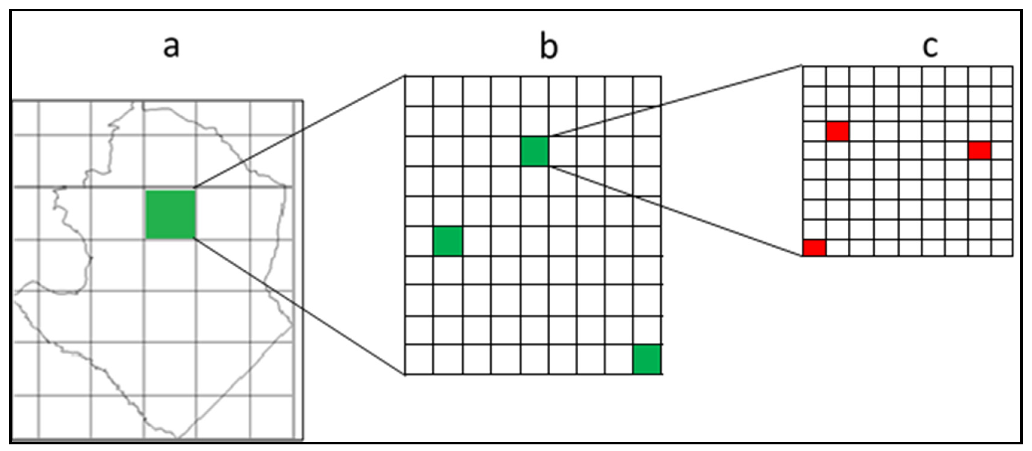
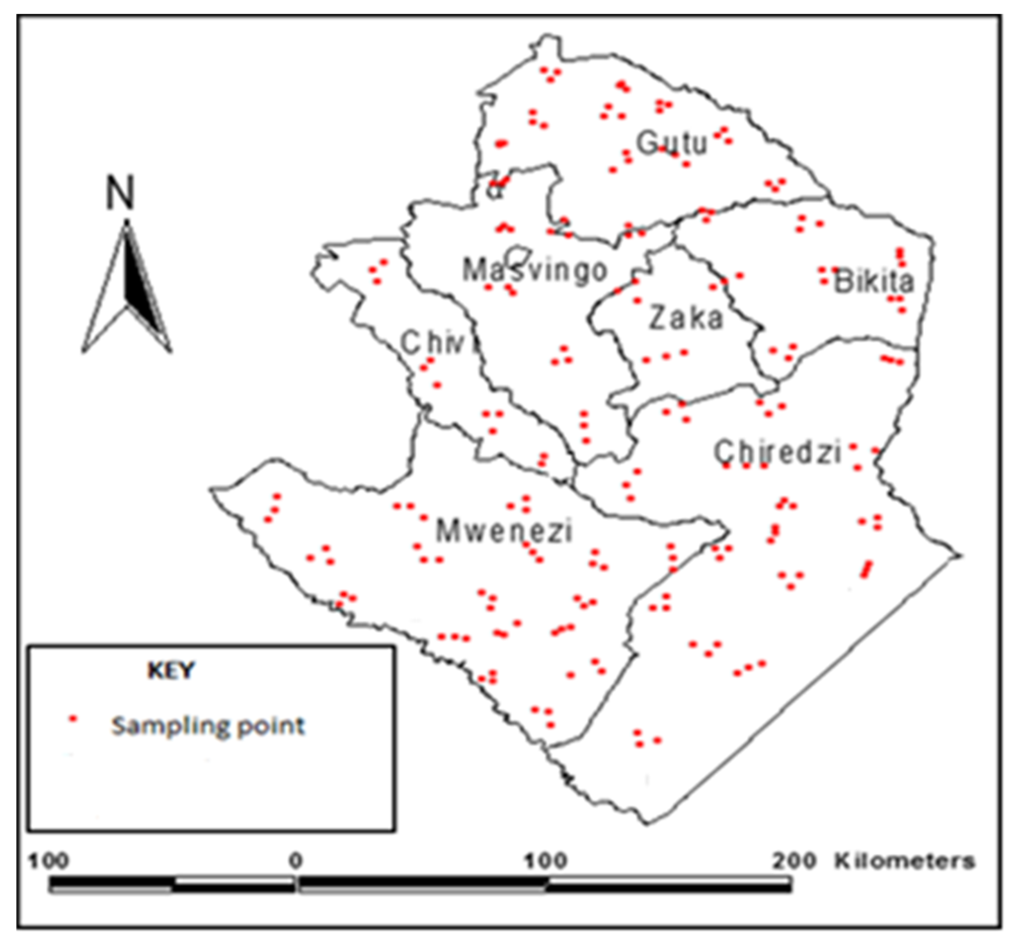
Data on plant species were collected from sampling points that were plotted throughout the province using a geographic information system (GIS)-based nonaligned block sampling design (Figure 2). This was preceded by plot size determination using the species-area method. This method involves plotting the number of species (species richness) identified in plots of a successively larger area so that the area enclosed by each one includes the area enclosed by the smaller one. Thus, 100 m², 400 m², 900 m², 1600 m², and 3600 m² plots were successively constructed to determine the optimum plot size. Species richness for each plot was recorded and 5, 7, 12, 12, 12 species were identified in the respective plots.

The optimum plot size is the one in which the number of species identified will not change with an increase in the size of the plot size. The 900 m² plot was identified as the optimum plot size. This falls within the recommended range of 400–2500 m², as suggested by Sutherland [32].

The GIS block sampling method uses a grid as a basic template, where sampling locations are randomly nested. The grid is a row and/or column that divides space into a unit or units of equal size. This method permits a multilevel assessment of variables at varied scales [31]. It takes into consideration regions with varying species, reducing sampling bias, as samples will be taken from each area of geographical difference. The sampling was done on a digital map of the study area using a step-by-step procedure as follows:

• Step 1: Grids of the same size were overlaid on the map of Masvingo province (Figure 2a). These grids were meant to divide the study area in a way that would allow samples to be obtained from all areas of geographic differences. All grids covering more than 40% of the province were selected. Each grid represents an area from which samples were taken. This makes the samples more representative as they cover all geographic areas throughout the study area. A total of 22 grids were selected.
• Step 2: Grids selected in step 1 were further subdivided into smaller grids of the same size (Figure 2b), from which 3 were randomly selected using the random point generator in ArcGIS. Thus, the number of selected grids increased to 66.
• Step 3: Grids in step 2 were further subdivided to come up with smaller grids of the same size (Figure 2c). Three smaller grids or sub-cells were randomly selected from each larger grid established in step 2. Thus, the number of selected grids increased to 198. These were the sampling points from which data were collected. From these selected grids, plots of 30 m x 30 m were established.

However, 4.04% of the plots were inaccessible due to steep mountain, forest thickets, deep water bodies and inaccessibility due to land designated as private property. Figure 3 shows the final sampling points in the whole province and the points that were inaccessible due to the given reasons.

The coordinates of the centre of the selected grids were entered into a Hand-held Global Positioning System (GPS) receiver, which was then used to navigate to the exact point locations at approximately 10 m error margin. Species counting was conducted within the study units (30 m × 30 m plots). To avoid double-counting and skipping of some species, the plots were subdivided into smaller units that made the counting of species easier. The subdivisions were done using a long cable.

All vegetative species within the confines of the established plots and quadrats were assessed and quantified to determine the diversity of species. The rooted frequency approach [31,33] was used on plots and quadrants that only had trees, herbs, and grass with roots found within the confines of those plots and quadrats. The sampling criteria for small plant species were different from that of tree species. Within the established plots, a radial arm was designed to facilitate the capture of variations in small, particularly grass, species within the 900 m² plot. Using the radial arm as the sampling framework, data on small plant species were collected from four quadrants: one from the centre, one from the northeast, one from the southeast, and the other from the northwest. The angle between arms was 120°, while the length of the arms was 12.2 m. To construct the radial arm, a campus was used to establish the azimuth of the arms. At the end of each arm and at the centre, a 1 m² quadrat was designed.

Small vegetation species within the 1 m × 1 m quadrats were assessed to determine species richness and evenness. These data were collected from the same plots four times over a year to cover all seasons (summer–November to March, post-summer–April to May, winter–June to August and post-winter–September to October) to monitor seasonal changes.

2.3. Satellite Image Processing

The images were acquired from the online Landsat archive via the GloVis web-link [34]. The year for the first imagery was determined by the availability of imagery with bands necessary to calculate NDVI. The Landsat images were calibrated to spectral radiance units (W m² sr¹ μm¹). The algorithm developed by Chander et al. [35] specifically for calibrating Landsat images and the calibration coefficients were provided together with the respective Landsat image files as metadata files as shown in Equation (1):

$$L\lambda =\left(\frac{Lmax\lambda -Lmin\mathsf{\lambda } }{Qcalmax-Qcalmin}\right)\left(Qcal-Qcalmin\right)+Lmin\mathsf{\lambda }$$

(1)

where L$\lambda$ is the quantized calibrated pixel value, Q_cal is the calibrated and quantized scaled radiance in units of digital numbers, Lmin_λ is the spectral radiance at QCAL = 0, Lmax_λ is the spectral radiance at QCAL = QCALMAX, and QCALMAX is the range of the rescaled radiance in digital numbers. The conversion from digital number (DN) to spectral radiance was done by implementing the algorithm developed by Chander et al. [35].

Landsat images (30 m spatial resolution) were to develop the normalised difference vegetation index (NDVI) data. NDVI is an arithmetical indicator used as a surrogate of plant biomass richness and health in remote sensing [36]. The NDVI uses the visible red band (0.4–0.7 μm) and near-infrared (NIR) bands (0.75–1.1 μm) of the electromagnetic spectrum to assess biomass richness (Equation (2)) [36].

$$\mathrm{NDVI}=\frac{NIR-R}{NIR+R}$$

(2)

High NDVI values represent rich and healthy vegetation (and thus high NDVI values indicate more species diversity), and negative NDVI values indicate the absence of vegetation [37]. In this study, the hypothesis is that, the higher the biomass, the greater the diversity of species. The NDVI values range from −1 through 0 to 1, where negative values are a sign that there is water, zero symbolises bare soil while positive values signal healthy vegetation. The NDVI was used over other indices because it has low sensitivity to soil differences, it is a function of a ratio; therefore, it is less sensitive to solar elevation, and it is very sensitive to the amount of green vegetation [38]. The NDVI was calculated for both dry and wet seasons between 1974 and 2014 using Landsat images.

2.4. Rainfall and Temperature Data

Rainfall and temperature data for weather stations within the province were obtained from the Zimbabwe Meteorological Services Department (ZMSD). The dataset obtained from the ZMSD was complemented by data from the National Centres for Environmental Information (NCEI), which is managed under National Oceanic and Atmospheric Administration (NOAA) programs for preserving, monitoring, and provision of climate and the historic weather data [39]. To be able to use both datasets, we compared through regression analysis, which showed a strong relationship (r = 0.95; R² = 0.91) for both variables.

2.5. Data Analysis

Exploratory and confirmatory data analysis approaches were used. The data were first subjected to normality tests using the Kolmogorov–Smirnov test to ascertain whether they deviate from a normal distribution or not [40]. Rainfall and temperature data, which constituted the time-series data, as well as plant species data were tested. This was done to determine whether the data satisfy the assumptions of parametric or nonparametric statistical analysis methods. Following the tests, nonparametric statistical analysis methods were used. Prior to trend analysis using the nonparametric Mann–Kendall test, climatological and plant species data were initially tested for autocorrelation to determine the need for prewhitening. Autocorrelation is the correlation of a time series with its past and future values [41]. Its detection would require the data to be prewhitened. Hamed and Rao [41] noted that the geophysical time series are frequently autocorrelated because of inertia or carryover processes in the physical system. This complicates the application of statistical tests by reducing the number of independent observations, thereby increasing the chances of detecting significant trends even if they are absent and vice versa. Prewhitening is the process of removing undesirable autocorrelations from time-series data prior to analysis. Thus, the data were prewhitened in Paleontological statistics (PAST 4.1) software (Palaeontologia Electronica, Oslo, Sweden) using the Autoregressive Integrated Moving Average (ARIMA) model [41]. The ARIMA model performs time-series forecasting and smoothening and projects the future values of a series based entirely on its inertia. It considers trends, seasonality, cycles, errors, and nonstationary aspects of a data set when making forecasts. It reduces residuals to white noise in the time series, hence removing the possibility of finding a significant trend in the Mann–Kendall test when there is no trend [42].

2.6. Trend Testing

The experiment tested if there was a significant change in precipitation, temperature, and species diversity over a 40 year period (1974–2014) using the Mann–Kendall trend test [43,44]. It is a nonparametric method commonly employed to detect monotonic trends in a series of environmental, climate, or hydrological data [45]. An add-in of Microsoft Excel, XLSTAT 2015.6 (Addinsoft Inc, New York, NY, USA), was used to carry out the test due to its ability to take into account and remove the effect of autocorrelations. The Mann–Kendall test statistic is calculated using Equation (3) [42].

$$S={\displaystyle \sum }_{k=1}^{n-1}{\displaystyle \sum }_{j=k+1}^{n}sgn \left(Xj-Xk\right)$$

(3)

where S is the Kendall score. Sgn (x) = (1 if x > 0, 0 if x = 0, −1 if x < 0) [43]

2.7. Interpolation

Species diversity data collected from the field and meteorological data from five weather stations were first interpolated using the Thiessen polygons approach in ArcGIS to ensure that all areas are represented by species diversity, temperature, and rainfall data. The area of the province was divided into several polygons, each around a measurement point. The weighted average of the measurements was taken based on the size of each one’s polygon. The weighted average was calculated using Equation (4) [46].

$$\overline{P}=\frac{P1A1+P2A2+P3A3\dots \dots \mathrm{..}PnAn}{A1+A2+A3\dots \dots \dots An}=\frac{{{\displaystyle \sum }}_{i=1}^{n}P1A1}{{{\displaystyle \sum }}_{i=1}^{n}A1}$$

(4)

where $\overline{P}$ is the weighted average, P’s are measurements, and A’s are areas of each polygon.

The interpolated data were then used for regression analysis of vegetative species and meteorological data to establish the relationship between climatic elements and species diversity.

2.8. Shannon Wiener Index (H)

Data on species abundance collected in the field were used to calculate vegetation species diversity using the Shannon index of diversity (H), which combines aspects of richness and evenness. It is an information statistics index, which measures the average degree of uncertainty in determining the genre of randomly chosen species from a collection of S species and N individuals [35]. The Shannon index is calculated using Equation (5) [35]:

$$H=-{\displaystyle \sum }_{i=1}^{s}Pi\ln P$$

(5)

where Pi is the proportion (n/N) of individuals of one species found (n) divided by the total number of individuals found (N), ln is the natural log, Σ is the sum of the calculations, and S is the number of species.

2.9. Questionnaire Surveys

Questionnaire surveys were administered to local communities at the household level. Questionnaire results were used to provide independent evidence of the relationships between species diversity and changes in climate variables. The survey data were also used to provide independent opinions on the trends of species diversity and climatic variables over the study period, as local communities generally have knowledge of the changes taking place in their localities. As the survey was essential for gathering information on the impact of climate change on vegetative species diversity, it was also used to complement data obtained through direct observation and remote sensing. The sampling criteria for the survey was similar to the one used for vegetative species assessment, where households were randomly chosen to participate in the surveys. A total of 189 questionnaires were administered, and the response rate was 95.24%.

Questionnaire data were collated in a grid and theme coding was performed in a spreadsheet (

Table 1. Score sheet for rating richness of indigenous, invasive species, and species diversity.

Year	Indigenous Species	Invasive Species	Plant Species Diversity
1974	9.5	0.6	9.3
1978	9.1	4.8	8.6
1982	9	6.1	8.3
1986	9	7.2	8.1
1990	8.8	7.9	7.9
1994	8.6	7.9	7.6
1998	6.8	8.0	6.8
2002	6.1	8.4	5.9
2006	5.9	8.7	5.6
2010	5	9.2	5.4
2014	4.3	9.8	5.2

Note: Richness score categories (0–10), 9–10—very high, 7–8—high, 5–6—medium, 2–4—low, 0–1—very low.

). For closed questions whose answers were ranked according to numerical scales, coding was done using the numerical scales of between 0 and 10. For open-ended questions, the responses were reviewed, and theme-coded. Survey data provided information that was used to determine changes in species richness and diversity over time. Thus, respondents provided scores on how they depicted and perceived species abundance, richness, and diversity. Table 1 is a sample of the instrument used to collect data and scoring richness and diversity for specified species category over the review period (1974–2014).

A score of 10 indicates that the respondent perceives the phenomenon to be very high, whilst a score of 0 indicates that the respondent perceives the phenomenon to be very little or absent. Summary statistics of scores from the 189 data points were computed in a spreadsheet. Specifically, average scores for each period depicted by a specific year and category were computed. Using the computed time-series data between 1974 and 2014, trendlines were produced in XLstats to determine changes over time.

A major limitation of the scoring procedure was the subjectivity of the scores as given by the respondents, as individuals differ in the way they perceive phenomena. In addition, the same individual’s perceptions may be altered by the environment, expectations, or circumstances during survey time. However, the large sample size used in this study helped in reducing the effect of individual biases. The use of quantitative methods was essential for reducing bias.

2.10. Key Informant Interviews

Key informant interviews were also conducted to infer data from important institutions and individuals involved in the management of natural vegetative species diversity and climate-change-related impacts, and provide independent evidence on the temporal and spatial relationships between climate variables and vegetation species diversity over time. The Ministry of Environment, Water, and Climate, the Climate change Office of Zimbabwe (COZ), the Forestry Commission of Zimbabwe (FCZ), the Environmental Management Agency (EMA) and the Meteorological Services Department (MSD) provided key personnel during this part of the study. Traditional leaders also provided vital information at the community level. Seven traditional leaders, one from each district, were interviewed.

The process involved asking questions whose responses provide answers to the research questions of the ongoing study. We used the semi-structured interview method in which the interview process was flexible, but at the same time, maintaining some structure over the concepts being discussed. An interview guide was used in the interview process.

3. Results and Discussion

3.1. Climate Change Trends in Masvingo Province

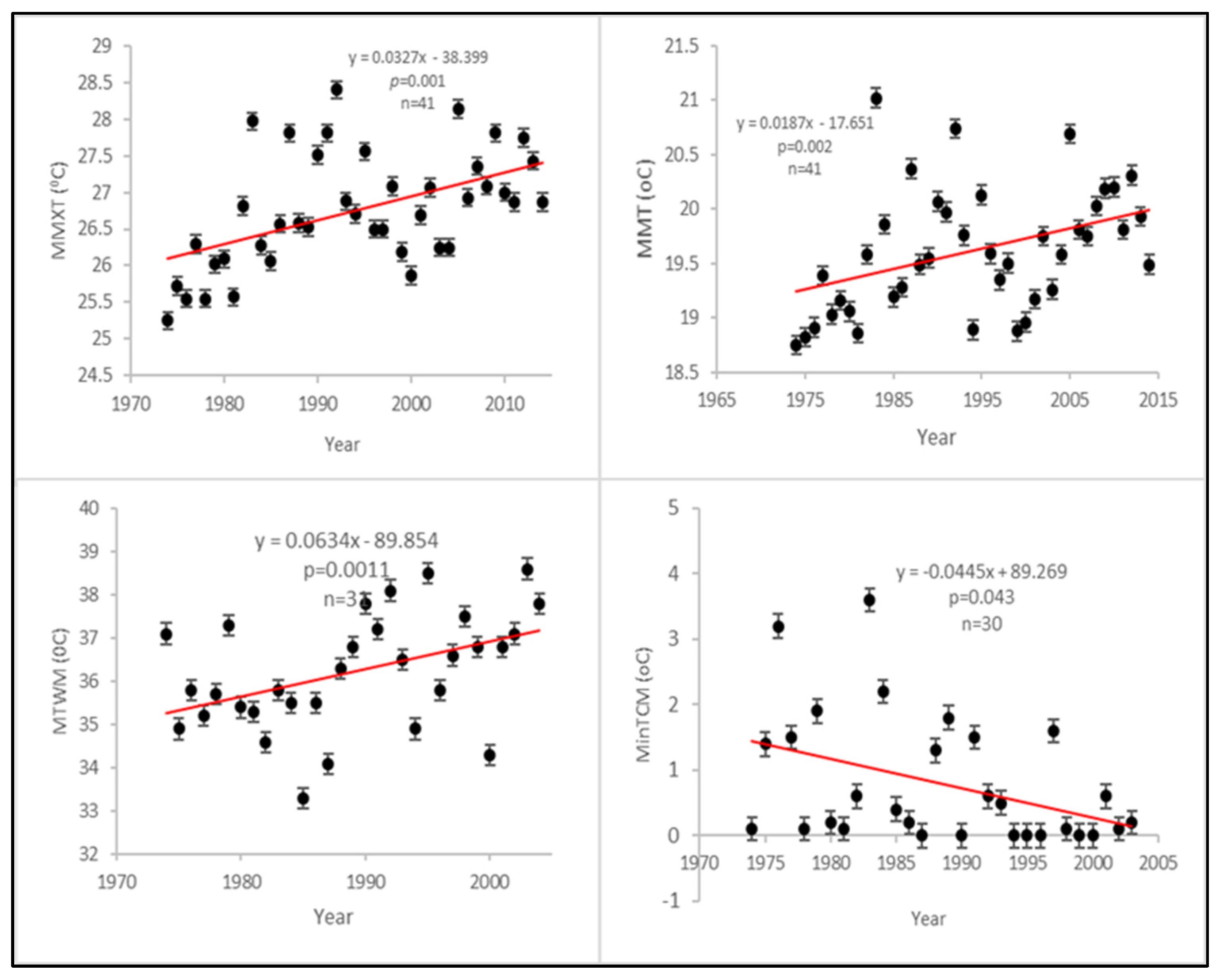
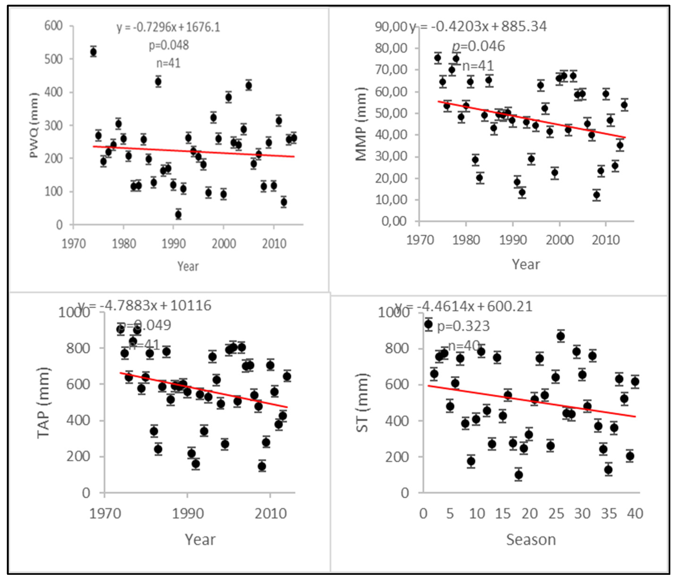
The trend of the 40 year temperature and rainfall data indicates that temperatures are rising and precipitation declining. About 87.5% of the assessed bioclimatic variables show a significant (p < 0.05) trend. Temperature-related variables such as mean monthly maximum temperatures (MMMT), mean monthly temperatures (MMT), maximum temperatures of the warmest month (MTWM), and minimum temperatures of the coldest month (MinTCM) show a generally increasing trend, indicating that the atmosphere is getting warmer with time. The increases in all the temperature-related variables are statistically significant. Precipitation variables such as total annual precipitation (TAP), mean monthly precipitation (MMP), precipitation of the warmest quarter (PWQ), and seasonal maximum precipitation (SMP) show a declining trend. This shows that, in general, there is a decline in the amount of rainfall received in the province over time. All the precipitation-related variables show a significant trend except SMP, although the trend is declining.

Table 2. Bioclimatic variables explaining climate change.

Climatic Variable	m + c	P-Value	Trend Description
Mean monthly max. temp	0.0327−38.399	0.001	Significant change/increasing trend
Mean monthly temp	0.0187−17.651	0.002	Significant change/increasing trend
Max. temp, warmest month	0.863−89.854	0.011	Significant change/increasing trend
Min. temp, coldest month	−0.0445 + 89.269	0.043	Significant change/declining trend
Total annual precipitation	−4.7883 + 10116	0.049	Significant change/declining trend
Mean monthly precipitation	0.4203 + 88534	0.046	Significant change/declining trend
Precipitation: warmest quarter	3.4206 + 7137.3	0.048	Significant change/declining trend
Seasonal max. precipitation	4.4614 + 60021	0.323 a	Not significant/declining trend

^a Trend not significant at α = 0.05.

shows the data and descriptions in the trends of 8 bioclimatic variables.

3.1.1. Temperature

Figure 4 shows 40 year trends for temperature-related variables (MMMT, MMT, MTWM, and MinTCM). The variables are important as they determine major climatic shifts over a long period of time. Given the role of temperature in plant metabolic processes, they are also important when determining the effects of climate change on plant species diversity.

There is a statistically significant (p = 0.001, α = 0.05) change in MMMT in the province. As shown in Figure 4, the linear model presents an increasing trend. An increase of about 0.33 °C is estimated over the 40 year period. The MMT also shows a significantly (P = 0.002, α = 0.05) increasing trend over the 40 years. The estimated MMT increased by 0.27 °C during the period under review. It is also observed that the trend for MTWM has increased over time and it is statistically significant (p = 0.011, α = 0.05). October is the warmest month of the year in this climatic region [47]. The selection of the month was based on a preliminary analysis of temperature characteristics of all months over a thirty-year period, i.e., 1974–2004. Furthermore, MinTCM shows that there is a significant (P = 0.043; α = 0.05) change of temperature regimes in the region.

The significant increase in temperature-related variables implies a warming climate in Masvingo Province. There has been an increase of +/− 0.33 °C per decade in monthly mean maximum temperatures and a +/− 0. 27 °C increase in monthly mean temperatures per decade. This is supported by previous studies that found out that there is a significant increase in temperatures in the interior of southern Africa [48]. These temperatures are projected to increase by 2 °C (using the Statistical Analogue Resembling Scheme (STARS) model) and by 3.5 °C (using the Regional Climate Model) by 2060 [48,49]. Therefore, the climate in the province is warming, as indicated by a significant increase in temperatures associated with prolonged occurrences of dry spells. The changing climatic regimes are resulting in ecological ramifications including plant species diversity modification.

3.1.2. Precipitation

Precipitation data in south-eastern Zimbabwe have been used to determine the statistical significance in the trends of different precipitation-related variables. The variables considered under precipitation include TAP, MMP, PWQ, and SMP. Figure 5 shows the trends for precipitation-related variables. These variables significantly depict climatic shifts over a long period of time.

Total annual precipitation, as the sum of all precipitation, received and recorded throughout the year, over a forty-year period, shows a statistically significant (P = 0.049, α = 0.05) declining trend. Moreover, the monthly mean precipitation shows a significantly (P = 0.046, α = 0.05) declining trend that depicts a changing climate. The warmest quarter is the three-month period, which receives the highest amount of radiation, and consequently, temperatures throughout the year. In the subtropical region in general and Zimbabwe in particular, this period falls between October and December [47]. Thus, precipitation data for the warmest quarter reveal a statistically significant (P = 0.048, α = 0.05) trend over a forty-year period. Precipitation data only for the rain season reveal that there is no significant (P = 0.323; α = 0.05) trend in the series. However, a gradually declining trend can be observed over time.

The analysis has shown a statistically significant decline in most of the precipitation-related variables such as the total annual rainfall, precipitation of the warmest quarter, and monthly mean precipitation. However, seasonal total precipitation shows a declining but not statistically significant trend. While the trend is not statistically significant, it contributes significantly to biodiversity changes, as also noted by the Intergovernmental Panel on Climate Change (IPCC) that ecosystem changes do not wait for precipitation changes to be significant, a slight shift in climatic elements may result in huge environmental consequences [6]. Nevertheless, the general precipitation-trend-related variables indicate that the province is getting drier over the long term. This dryness is causing significant modification of plant species.

3.2. Climate Change and Plant Species Diversity

The plant species in Masvingo are vulnerable to climatic perturbations. The regression results (

Table 3. Regression vegetative species diversity results by climate variables from the 198 observations.

Regression Variables	m + c	Correlation Coefficient (r)	p Value	R2
H and mean monthly precipitation	0.0339–0.6662	0.794	<0.001	0.6736
H and precipitation: warmest quarter	0.0005–0.2338	0.734	<0.001	0.6455
H and seasonal max. precipitation	0.0049–0.3063	0.702	<0.001	0.5841
H and total annual precipitation	0.0036–0.0413	0.703	<0.001	0.6261
H and min. temp, coldest month	0.2651 + 1.4877	0.706	<0.001	0.4979
H and max. temp, warmest month	−0.0893 + 5.6494	−0.799	<0.001	0.6706
H and mean monthly max. temp	−0.0799 + 4.4873	−0.776	<0.001	0.6223
H and mean monthly temp	−0.0439 + 3.4388	−0.126	<0.001	0.6943

) for climate variables and species diversity (H) show correlations between plant species diversity and climate.

For precipitation-related variables, the monthly mean precipitation best explains vegetative species diversity, while for temperature-related variables, monthly mean temperatures have the highest coefficient of determination. The relationship between climatic variables and species diversity suggests that a change in climatic variables can result in a change in species diversity.

3.2.1. Plant Species Diversity and Precipitation-Related Variables

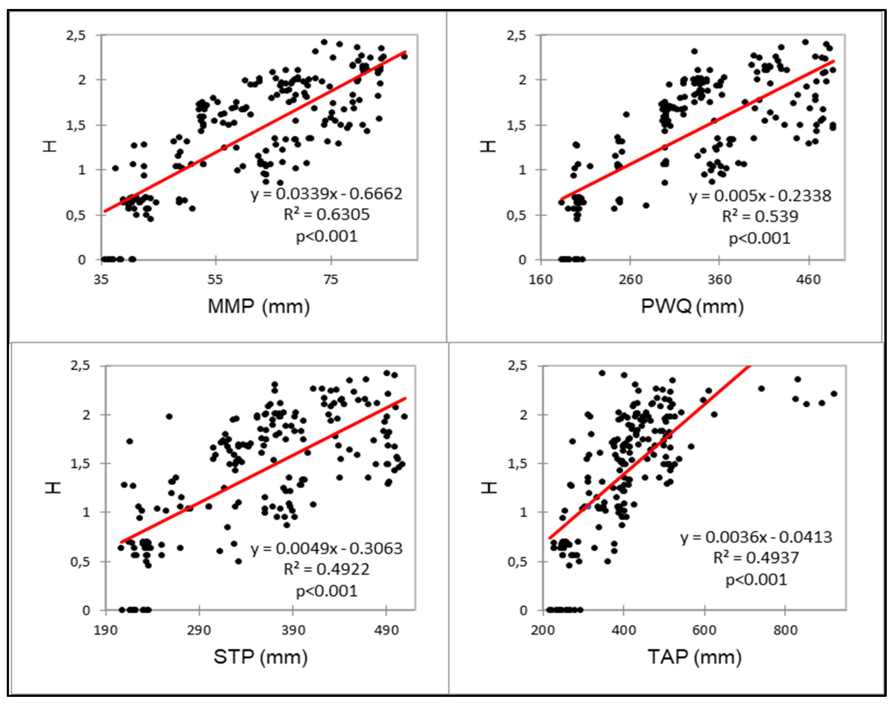
Results of the regression analysis of the Shannon diversity index (H) versus Precipitation-related climate variables (MMP, TAP, SMP, and PWQ) are shown in Figure 6. The four precipitation-related climate variables correlate with the diversity of vegetative species. Sixty-seven percent of plant species diversity is significantly predicted by MMP (P < 0.001).

There is a positive correlation (r = 0.734) between H and PWQ (October to December). The results show that, as precipitation of the warmest quarter increases, vegetative species diversity also increases. In addition, SMP seems to play an important role in determining the diversity of plant species in Masvingo Province. This is shown by the positive correlation (r = 0.702) between H and SMP. As shown in Figure 6, 49% of vegetative species diversity is significantly (p < 0.001) explained by SMP. Regression of the two variables shows that, as seasonal total precipitation increases, species diversity also increases. Furthermore, TAP and species diversity have a strong positive correlation (r = 0.703). About 63% of vegetative species diversity in the province is significantly (P < 0.001) explained by TAP (Figure 6).

3.2.2. Vegetative Species Diversity and Temperature-Related Variables

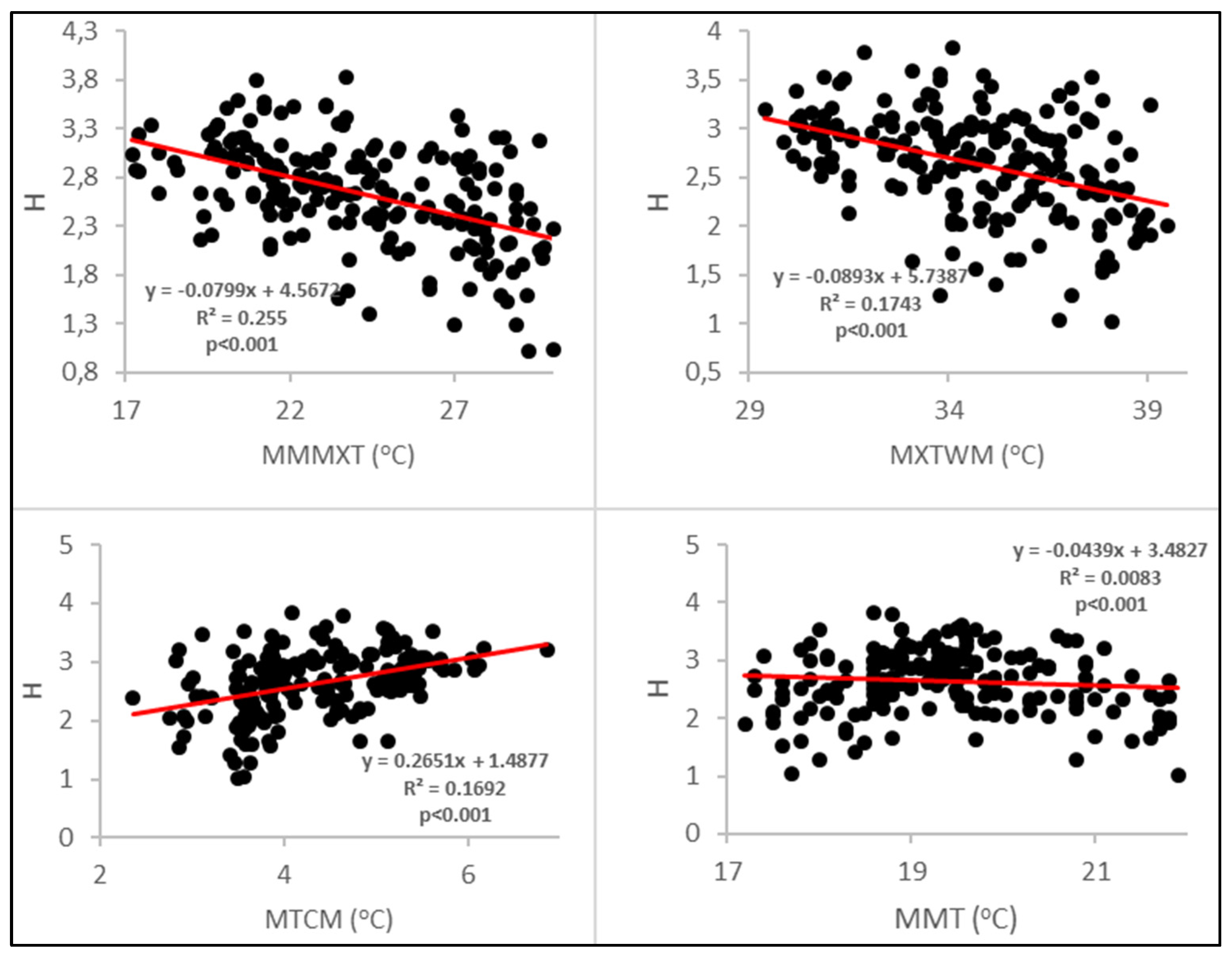
The linear regression of plant species diversity (H) by temperature-related climate change variables (Figure 7) shows correlation. There is a strong negative (−0.799) correlation between H and maximum temperatures of the warmest month (MTWM).

As shown in Figure 7, about 67% of vegetative species diversity is significantly (P < 0.001) explained by MTWM. An increase in MTWM is related to a decrease in plant species diversity. At temperatures of 39 °C and above, the diversity of species is extremely low. A positive correlation (r = 0.706) between H and MinTCM is also shown. About 49% of the vegetative species diversity is significantly (P < 0.001) explained by MinTCM. Similarly, MMMT explains plant species diversity. There is a strong negative correlation (r = −0.776). Also, 62% of vegetative species diversity in the province can be explained by MMT. Thus, an increase in MMT is associated with a decrease in H.

3.3. Diversity Dynamics Depicted Through Remote Sensing

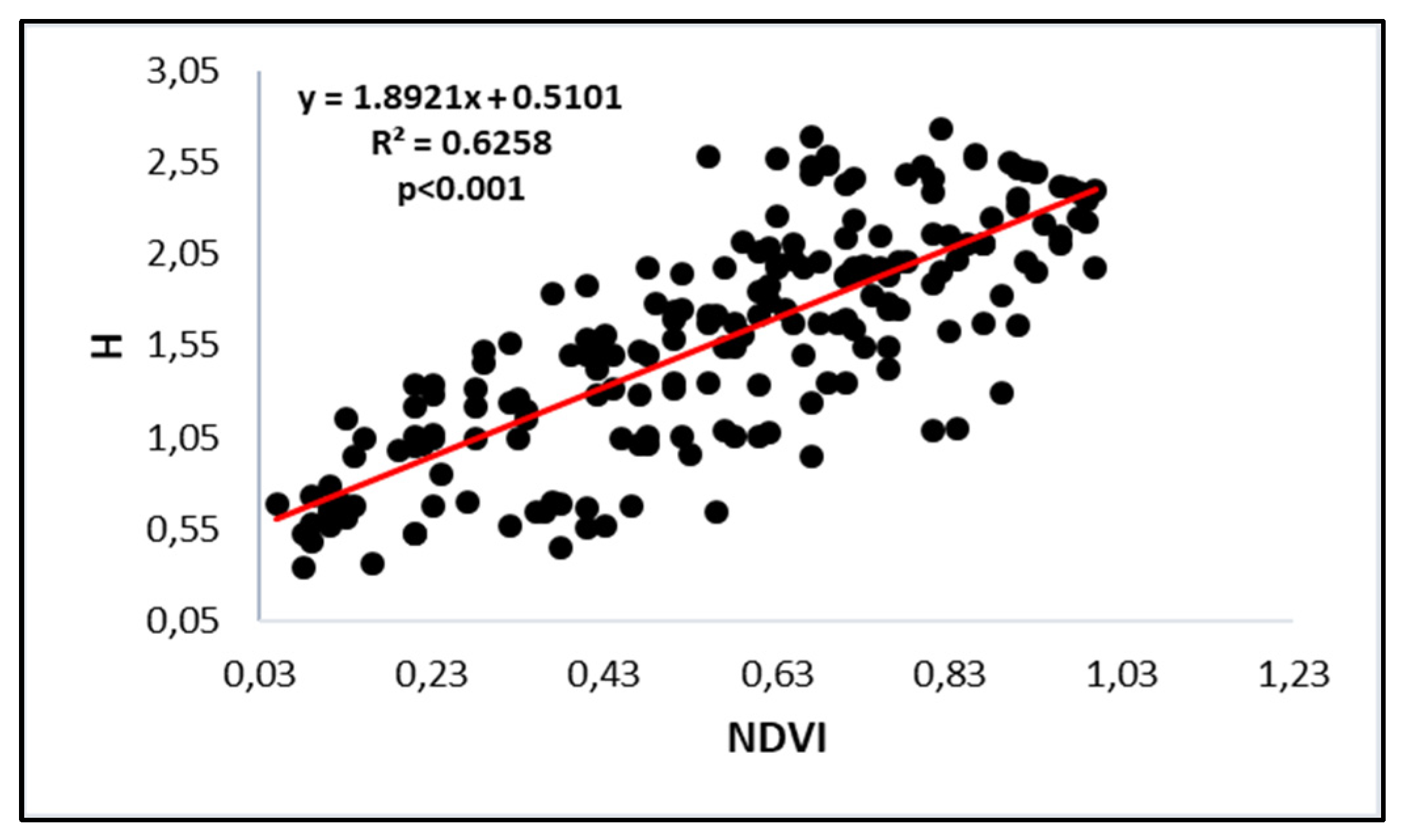
The relationship between NDVI and plant species diversity (H) was also assessed. Results show that NDVI has a positive linear response to plant species diversity (Figure 8). There is a strong (r = 0.79) correlation between NDVI and vegetative species diversity. NDVI explains 62% of vegetative species diversity. These results imply that NDVI can be used as a surrogate for vegetative species diversity. An increase in vegetative species diversity corresponds with an increase in NDVI, but the increase does not continue beyond 2.3 of H.

The decrease in diversity as temperatures increase implies that some vegetative species’ tolerance decreases with an increase in maximum temperatures of the warmest month, as also suggested by Gwitira et al. [47]. Furthermore, the results indicate that the regression analysis between NDVI and plant species richness is consistent with the Spectral Variation Hypothesis (SVH), which envisages a direct correlation between differences in reflectance of remote sensing images with environmental heterogeneity and beta diversity [50]. Thus, the hypothesis asserts that spectral heterogeneity is related to spatial ecological heterogeneity and thus to vegetative species diversity.

3.4. Changes in Species Diversity Between 1974 and 2014

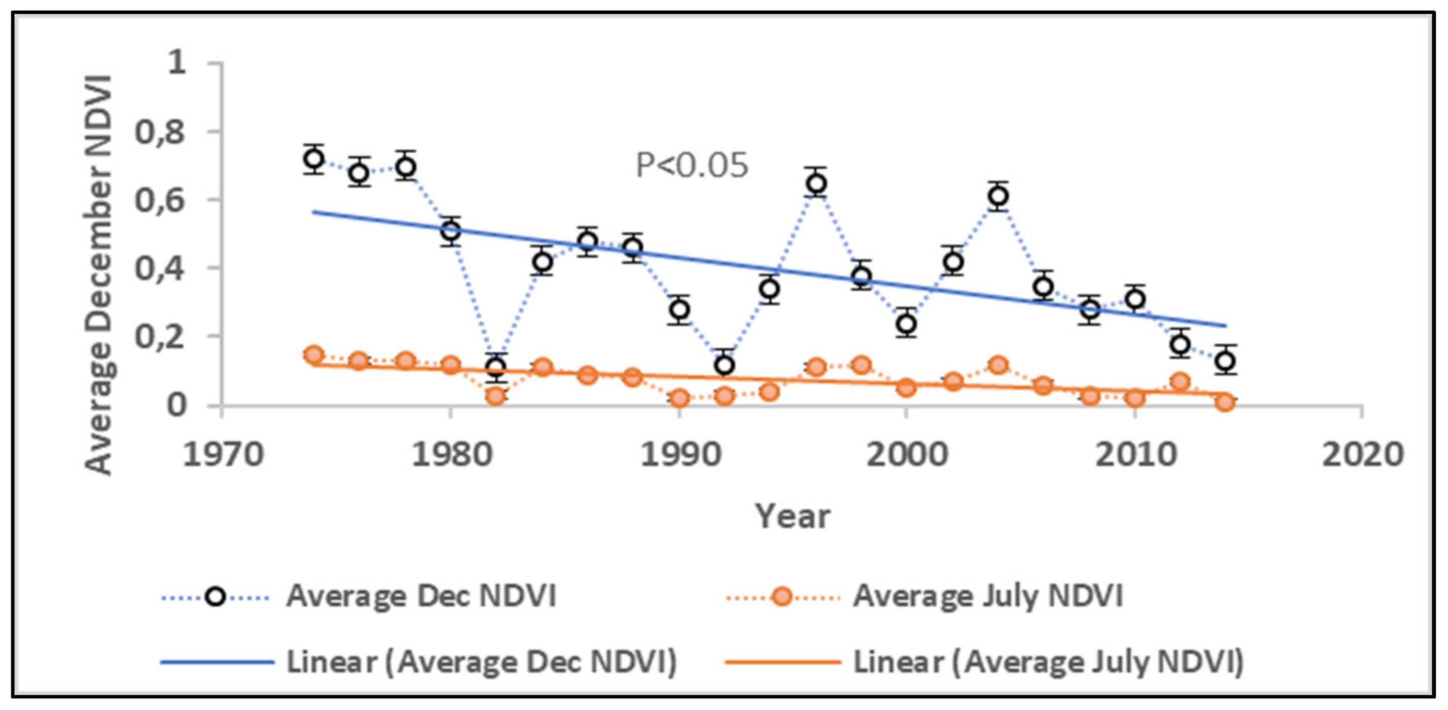
There is a significant (P = 0.041, α = 0.05) decrease in average December NDVI over the period 1974–2014 (Figure 9). However, the trend for average July NDVI is not significant (P = 0.062, α = 0.05) but declining. Given the correlation between NDVI and H, we used NDVI as a surrogate for H. Thus, a decrease in NDVI depicts a decrease in species diversity. Although 0.062 is not statistically significant at α = 0.05, it is at α = 0.1; there is clearly evidence that NDVI is related to diversity.

Despite the evidence from the analysis, respondents in the study area (92.3%) indicated that they have observed a decrease in the diversity of species over time. They indicated that there are some endemic species whose population has declined significantly, while others have become extinct due to climate changes as well as changes in land-use practices. Amongst the most affected species were herbaceous and graminoid species such as Digitaria penzii, Cynodon dactylon, Eragrostis trichophora, D. penzii, E. trichophora, and Hyperthelia dissoluta, Urochloa mozambicensis, Heteropogon contortus. Tree species such as the Julbernardia globiflora, Brachystegia spiciformis, Parinari curatellifolia Burkea Africana, Terminalia sericea, and Colophospermum Mopane were reported to be affected through logging by communities. The logging is presumed to be an indirect impact of a climate-change-constrained environment, as respondents confirmed that logging is generally observed as one of the adaptation mechanisms.

3.5. Evidence of Changes in Vegetative Species Diversity Through Interviews

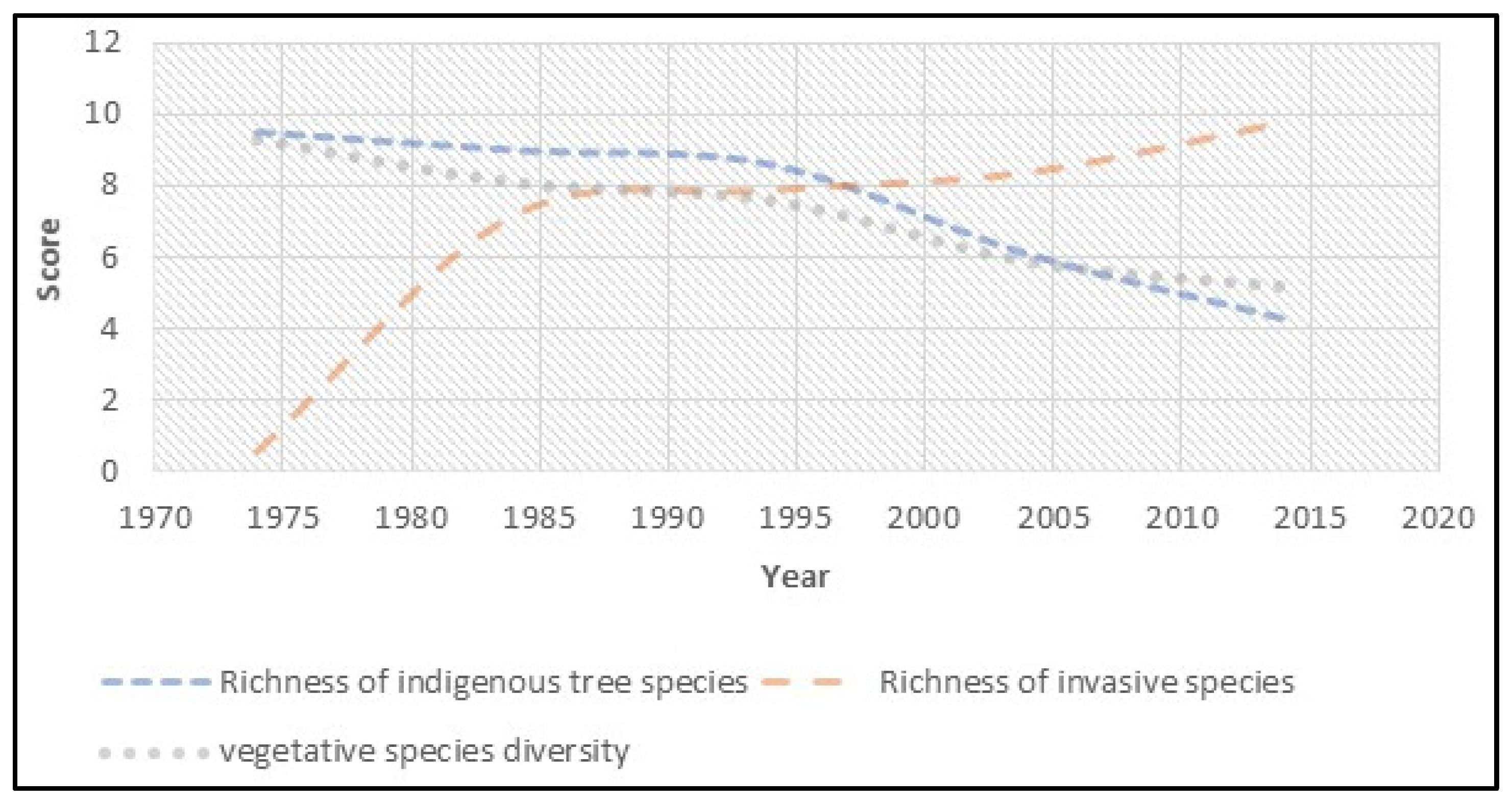
Results from the questionnaire survey and interviews complemented the results from remote sensing and statistical analysis by also showing changes in vegetative species diversity in the study area over time, as shown in Figure 10. Indigenous tree species and vegetative species diversity have been declining steadily since 1975 to date, at a time when invasive species have been increasing (Figure 10).

Scores depict the level of a phenomenon as observed by people residing in the province. A high score is reflective of a high level of a specified phenomenon. Invasive species richness has been increasing in the province since 1974, although the increase stabilised since 1985. While there has been an increase in invasive alien species, indigenous tree species richness has been decreasing, the steepest decline being observed from 1994 to 2014.

Although the study considered the drivers of spatial variability in vegetative plant diversity as proxies of the drivers of temporal variability through vegetation indices, it recognises the influence of other factors such as the long (decadal to multidecadal) life spans of trees, stability of soil properties, dispersal limitations that collectively drive species composition in a given location [51,52]. Although future research should also focus on the influence of these other important factors influencing changes on plant species diversity, recent studies that analysed the turnover of species diversity along an ecological succession since the melting of glaciers [52], and along a mountain treeline shift [53], showed that space is a reliable substitution of time.

The use of spatial variation over time has been widely used in ecological processes and in understanding long-term ecological dynamics across sites that vary in environmental conditions [54]. Studies have also extrapolated temporal dynamics in species diversity by comparing multiple sites in a region, particularly in gradient analyses, and have shown the reliability of space-for-time substitution [55,56,57,58]. Other studies that support the methodology used in this study include those that applied space-for-time-substitution in biodiversity modelling to project climate-driven changes in species distributions, species richness, and compositional turnover [59,60]. These studies support the judicious use of space-for-time substitution in modelling plant species diversity responses to climate change.

4. Conclusions

Climate change denoted by long-term changes in temperature and precipitation, as well as extreme meteorological events, is influencing the diversity of plant species diversity of savanna ecosystems in Masvingo province. Changes in precipitation and temperature are reducing the available water resources through prolonged drought and extreme heatwaves, resulting in the proliferation of climate-sensitive species, causing their desiccation and extinction. Drying environments are favouring invasive alien species, exacerbating the extinction of some savanna species. Herbal and grass species have been the most affected. The net resultant effect is the loss of plant species diversity. Thus, climatic perturbations are directly and indirectly influencing plant species diversity loss through environmental modifications due to climate change. Environmental changes are creating unfavourable conditions for the continued production and health of specific species. Consequently, plant species are responding differently, as evidenced by changes in species range, abundance, or in the timing of life-cycle events and diversity patterns. Although other factors such as edaphic changes, veld fires, and land-use changes are also impacting plant species diversity in the savanna region, climate change remains the main reason behind the reduction in plant species diversity in this ecosystem. Further studies are required to focus on specific plant species using global circulation models and modelling techniques to assess the changes in plant species over time and under different scenarios.

References

1. Bellard, C.; Bertelsmeier, C.; Leadley, P.; Thuiller, W.; Courchamp, F. Impacts of climate change on the future of biodiversity. Ecol. Lett. 2012, 15, 365–377. [Google Scholar] [CrossRef] [PubMed] [Green Version]
2. Henson, S.A.; Beaulieu, C.; Ilyina, T.; John, J.G.; Long, M.; Séférian, R.; Tjiputra, J.; Sarmiento, J.L. Rapid emergence of climate change in environmental drivers of marine ecosystems. Nat. Commun. 2017, 8, 14682. [Google Scholar] [CrossRef]
3. Liu, H.; Mi, Z.; Lin, L.; Wang, Y.; Zhang, Z.; Zhang, F.; Wang, H.; Liu, L.; Zhu, B.; Cao, G. Shifting plant species composition in response to climate change stabilizes grassland primary production. Proc. Natl. Acad. Sci. USA 2018, 115, 4051–4056. [Google Scholar] [CrossRef] [PubMed] [Green Version]
4. Jewitt, D.; Erasmus, B.F.; Goodman, P.S.; O’Connor, T.G.; Hargrove, W.W.; Maddalena, D.M.; Witkowski, E.T. Climate-induced change of environmentally defined floristic domains: A conservation based vulnerability framework. Appl. Geogr. 2015, 63, 33–42. [Google Scholar] [CrossRef]
5. Ummenhofer, C.C.; Meehl, G.A. Extreme weather and climate events with ecological relevance: A review. Philos. Trans. R. Soc. B Biol. Sci. 2017, 372, 20160135. [Google Scholar] [CrossRef] [PubMed]
6. Handmer, J.; Honda, Y.; Kundzewicz, Z.W.; Arnell, N.; Benito, G.; Hatfield, J.; Mohamed, I.F.; Peduzzi, P.; Wu, S.; Sherstyukov, B. Changes in impacts of climate extremes: Human systems and ecosystems. In Managing the Risks of Extreme Events and Disasters to Advance Climate Change Adaptation, Special Report of the Intergovernmental Panel on Climate Change (IPCC); IPCC: Cambridge, UK, 2012; pp. 231–290. [Google Scholar]
7. Banerjee, K.; Gatti, R.C.; Mitra, A. Climate change-induced salinity variation impacts on a stenoecious mangrove species in the Indian Sundarbans. Ambio 2017, 46, 492–499. [Google Scholar] [CrossRef] [PubMed] [Green Version]
8. Abreu, R.C.; Hoffmann, W.A.; Vasconcelos, H.L.; Pilon, N.A.; Rossatto, D.R.; Durigan, G. The biodiversity cost of carbon sequestration in tropical savanna. Sci. Adv. 2017, 3, e1701284. [Google Scholar] [CrossRef] [Green Version]
9. Tsalyuk, M.; Kelly, M.; Getz, W.M. Improving the prediction of African savanna vegetation variables using time series of MODIS products. ISPRS J. Photogramm. Remote Sens. 2017, 131, 77–91. [Google Scholar] [CrossRef] [Green Version]
10. Nhamo, L.; Magidi, J.; Dickens, C. Determining wetland spatial extent and seasonal variations of the inundated area using multispectral remote sensing. Water SA 2017, 43, 543–552. [Google Scholar] [CrossRef] [Green Version]
11. FAO. The State of Food and Agriculture. Climate Change, Agriculture and Food Security; Food and Agriculture Organization of the United Nations (FAO): Rome, Italy, 2016; p. 194. [Google Scholar]
12. Devine, A.P.; McDonald, R.A.; Quaife, T.; Maclean, I.M. Determinants of woody encroachment and cover in African savannas. Oecologia 2017, 183, 939–951. [Google Scholar] [CrossRef] [Green Version]
13. Timpane-Padgham, B.L.; Beechie, T.; Klinger, T. A systematic review of ecological attributes that confer resilience to climate change in environmental restoration. PLoS ONE 2017, 12, e0173812. [Google Scholar] [CrossRef] [PubMed] [Green Version]
14. Parmesan, C.; Yohe, G. A globally coherent fingerprint of climate change impacts across natural systems. Nature 2003, 421, 37. [Google Scholar] [CrossRef] [PubMed]
15. Gatti, R.C.; Di Paola, A.; Bombelli, A.; Noce, S.; Valentini, R. Exploring the relationship between canopy height and terrestrial plant diversity. Plant Ecol. 2017, 218, 899–908. [Google Scholar] [CrossRef]
16. Walther, G.-R.; Post, E.; Convey, P.; Menzel, A.; Parmesan, C.; Beebee, T.J.; Fromentin, J.-M.; Hoegh-Guldberg, O.; Bairlein, F. Ecological responses to recent climate change. Nature 2002, 416, 389. [Google Scholar] [CrossRef] [PubMed]
17. Hillebrand, H.; Blasius, B.; Borer, E.T.; Chase, J.M.; Downing, J.A.; Eriksson, B.K.; Filstrup, C.T.; Harpole, W.S.; Hodapp, D.; Larsen, S. Biodiversity change is uncoupled from species richness trends: Consequences for conservation and monitoring. J. Appl. Ecol. 2018, 55, 169–184. [Google Scholar] [CrossRef] [Green Version]
18. Dobson, A. Monitoring global rates of biodiversity change: Challenges that arise in meeting the Convention on Biological Diversity (CBD) 2010 goals. Philos. Trans. R. Soc. B Biol. Sci. 2005, 360, 229–241. [Google Scholar] [CrossRef] [Green Version]
19. Tittensor, D.P.; Walpole, M.; Hill, S.L.; Boyce, D.G.; Britten, G.L.; Burgess, N.D.; Butchart, S.H.; Leadley, P.W.; Regan, E.C.; Alkemade, R. A mid-term analysis of progress toward international biodiversity targets. Science 2014, 346, 241–244. [Google Scholar] [CrossRef] [PubMed]
20. Hoehndorf, R.; Alshahrani, M.; Gkoutos, G.V.; Gosline, G.; Groom, Q.; Hamann, T.; Kattge, J.; de Oliveira, S.M.; Schmidt, M.; Sierra, S. The flora phenotype ontology (FLOPO): Tool for integrating morphological traits and phenotypes of vascular plants. J. Biomed. Semant. 2016, 7, 65. [Google Scholar] [CrossRef] [Green Version]
21. Kattge, J.; Diaz, S.; Lavorel, S.; Prentice, I.C.; Leadley, P.; Bönisch, G.; Garnier, E.; Westoby, M.; Reich, P.B.; Wright, I.J. TRY–a global database of plant traits. Glob. Chang. Biol. 2011, 17, 2905–2935. [Google Scholar] [CrossRef]
22. Kuenzer, C.; Ottinger, M.; Wegmann, M.; Guo, H.; Wang, C.; Zhang, J.; Dech, S.; Wikelski, M. Earth observation satellite sensors for biodiversity monitoring: Potentials and bottlenecks. Int. J. Remote Sens. 2014, 35, 6599–6647. [Google Scholar] [CrossRef] [Green Version]
23. Chapungu, L.; Nhamo, L.; Gatti, R.C. Estimating biomass of savanna grasslands as a proxy of carbon stock using multispectral remote sensing. Remote Sens. Appl. Soc. Environ. 2020, 17, 100275. [Google Scholar] [CrossRef]
24. Pettorelli, N.; Ryan, S.; Mueller, T.; Bunnefeld, N.; Jędrzejewska, B.; Lima, M.; Kausrud, K. The Normalized Difference Vegetation Index (NDVI): Unforeseen successes in animal ecology. Clim. Res. 2011, 46, 15–27. [Google Scholar] [CrossRef]
25. Wang, R.; Gamon, J.; Montgomery, R.; Townsend, P.; Zygielbaum, A.; Bitan, K.; Tilman, D.; Cavender-Bares, J. Seasonal variation in the NDVI–species richness relationship in a prairie grassland experiment (Cedar Creek). Remote Sens. 2016, 8, 128. [Google Scholar] [CrossRef] [Green Version]
26. Walker, R.; Stoms, D.; Estes, J.; Cayocca, K. Relationships between Biological Diversity and Multi-temporal Vegetation Index Data in California; American Society for Photogrametry & Remote Sensing (ASPRS) Convention: Albuquerque, NM, USA, 1992; p. 562. [Google Scholar]
27. Jørgensen, A.; Nøhr, H. The use of satellite images for mapping of landscape and biological diversity in the Sahel. Int. J. Remote Sens. 1996, 17, 91–109. [Google Scholar] [CrossRef]
28. Rafique, R.; Zhao, F.; de Jong, R.; Zeng, N.; Asrar, G. Global and regional variability and change in terrestrial ecosystems net primary production and NDVI: A model-data comparison. Remote Sens. 2016, 8, 177. [Google Scholar] [CrossRef] [Green Version]
29. Zhang, M.; Lin, H.; Wang, G.; Sun, H.; Cai, Y. Estimation of Vegetation Productivity Using a Landsat 8 Time Series in a Heavily Urbanized Area, Central China. Remote Sens. 2019, 11, 133. [Google Scholar] [CrossRef] [Green Version]
30. Skidmore, A.; Oindo, B.; Said, M. Biodiversity assessment by remote sensing. In Proceedings of the 30th International symposium on remote sensing of the environment: Information for risk management and sustainable development, Honolulu, Hawai, 10–14 November 2003; p. 4. [Google Scholar]
31. Chapungu, L.; Yekeye, T. Estimating tree species diversity in small scale farming areas for effective environmental management. The case of Bindura and Shamva Districts, Zimbabwe. Sacha J. Environ. Stud. 2013, 3, 23–33. [Google Scholar]
32. Sutherland, W.J. Ecological Census Techniques: A Handbook; Cambridge University Press: Cambridge, UK, 2006. [Google Scholar]
33. Ludwig, J.A.; Reynolds, J. Statistical Ecology: A Primer in Methods and Computing; John Wiley & Sons: New York, NY, USA, 1988; Volume 1. [Google Scholar]
34. GloVis. Global Visualization Viewer (GloVis); U.S. Department of the Interior, U.S. Geological Survey: Reston, VA, USA, 2005. Available online: https://glovis.usgs.gov/ (accessed on 17 March 2020).
35. Chander, G.; Markham, B.L.; Helder, D.L. Summary of current radiometric calibration coefficients for Landsat MSS, TM, ETM+, and EO-1 ALI sensors. Remote Sens. Environ. 2009, 113, 893–903. [Google Scholar] [CrossRef]
36. Tucker, C.J. Red and photographic infrared linear combinations for monitoring vegetation. Remote Sens. Environ. 1979, 8, 127–150. [Google Scholar] [CrossRef] [Green Version]
37. Mpandeli, S.; Nhamo, L.; Moeletsi, M.; Masupha, T.; Magidi, J.; Tshikolomo, K.; Liphadzi, S.; Naidoo, D.; Mabhaudhi, T. Assessing climate change and adaptive capacity at local scale using observed and remotely sensed data. Weather Clim. Extrem. 2019, 26, 100240. [Google Scholar] [CrossRef]
38. Matsushita, B.; Yang, W.; Chen, J.; Onda, Y.; Qiu, G. Sensitivity of the enhanced vegetation index (EVI) and normalized difference vegetation index (NDVI) to topographic effects: A case study in high-density cypress forest. Sensors 2007, 7, 2636–2651. [Google Scholar] [CrossRef] [PubMed] [Green Version]
39. Young, A.H.; Knapp, K.R.; Inamdar, A.; Rossow, W.B.; Hankins, W. The International Satellite Cloud Climatology Project, H-Series Climate Data Record Product; Earth System Science Data: Asheville, NC, USA, 2017. [Google Scholar] [CrossRef]
40. Massey, F.J., Jr. The Kolmogorov-Smirnov test for goodness of fit. J. Am. Stat. Assoc. 1951, 46, 68–78. [Google Scholar] [CrossRef]
41. Hamed, K.H.; Rao, A.R. A modified Mann-Kendall trend test for autocorrelated data. J. Hydrol. 1998, 204, 182–196. [Google Scholar] [CrossRef]
42. Von Storch, H. Misuses of statistical analysis in climate research. In Analysis of Climate Variability; von Storch, H., Navarra, A., Eds.; Springer: Berlin/Heidelberg, Germany, 1999; pp. 11–26. [Google Scholar]
43. Mann, H.B. Nonparametric tests against trend. Econom. J. Econom. Soc. 1945, 13, 245–259. [Google Scholar] [CrossRef]
44. Kendall, M.G. Rank Correlation Methods; Griffin: London, UK, 1945. [Google Scholar]
45. Ahmad, I.; Tang, D.; Wang, T.; Wang, M.; Wagan, B. Precipitation trends over time using Mann-Kendall and spearman’s rho tests in swat river basin, Pakistan. Adv. Meteorol. 2015, 2015, 15. [Google Scholar] [CrossRef] [Green Version]
46. Hoke, M.; Ross, B.; Wickesberg, R.; Lütkenhöner, B. Weighted averaging—theory and application to electric response audiometry. Electroencephalogr. Clin. Neurophysiol. 1984, 57, 484–489. [Google Scholar] [CrossRef]
47. Gwitira, I.; Murwira, A.; Shekede, M.D.; Masocha, M.; Chapano, C. Precipitation of the warmest quarter and temperature of the warmest month are key to understanding the effect of climate change on plant species diversity in S outhern A frican savannah. Afr. J. Ecol. 2014, 52, 209–216. [Google Scholar] [CrossRef]
48. Lutz, J.; Volkholz, J.; Gerstengarbe, F.-W. Climate projections for southern Africa using complementary methods. Int. J. Clim. Chang. Strateg. Manag. 2013, 5, 130–151. [Google Scholar] [CrossRef]
49. Kusangaya, S.; Warburton, M.L.; Van Garderen, E.A.; Jewitt, G.P. Impacts of climate change on water resources in southern Africa: A review. Phys. Chem. EarthParts A/B/C 2014, 67, 47–54. [Google Scholar] [CrossRef]
50. Rocchini, D.; Balkenhol, N.; Carter, G.A.; Foody, G.M.; Gillespie, T.W.; He, K.S.; Kark, S.; Levin, N.; Lucas, K.; Luoto, M. Remotely sensed spectral heterogeneity as a proxy of species diversity: Recent advances and open challenges. Ecol. Inform. 2010, 5, 318–329. [Google Scholar] [CrossRef]
51. Andrus, R.A.; Harvey, B.J.; Rodman, K.C.; Hart, S.J.; Veblen, T.T. Moisture availability limits subalpine tree establishment. Ecology 2018, 99, 567–575. [Google Scholar] [CrossRef] [PubMed]
52. Russell, A.E.; Kivlin, S.N.; Hawkes, C.V. Tropical tree species effects on soil pH and biotic factors and the consequences for macroaggregate dynamics. Forests 2018, 9, 184. [Google Scholar] [CrossRef] [Green Version]
53. Cazzolla Gatti, R.; Dudko, A.; Lim, A.; Velichevskaya, A.I.; Lushchaeva, I.V.; Pivovarova, A.V.; Volkov, I.V. The last 50 years of climate-induced melting of the Maliy Aktru glacier (Altai Mountains, Russia) revealed in a primary ecological succession. Ecol. Evol. 2018, 8, 7401–7420. [Google Scholar] [CrossRef] [PubMed]
54. Cazzolla Gatti, R.; Callaghan, T.; Velichevskaya, A.; Dudko, A.; Fabbio, L.; Battipaglia, G.; Liang, J. Accelerating upward treeline shift in the Altai Mountains under last-century climate change. Sci. Rep. 2019, 9, 1–13. [Google Scholar] [CrossRef]
55. Fukami, T.; Wardle, D.A. Long-term ecological dynamics: Reciprocal insights from natural and anthropogenic gradients. Proc. R. Soc. B Biol. Sci. 2005, 272, 2105–2115. [Google Scholar] [CrossRef] [Green Version]
56. Garnier, E.; Cortez, J.; Billès, G.; Navas, M.L.; Roumet, C.; Debussche, M.; Laurent, G.; Blanchard, A.; Aubry, D.; Bellmann, A.; et al. Plant functional markers capture ecosystem properties during secondary succession. Ecology. 2004, 85, 2630–2637. [Google Scholar] [CrossRef]
57. Lavorel, S.; Garnier, E. Predicting changes in community composition and ecosystem functioning from plant traits: Revisiting the Holy Grail. Functional Ecology. 2002, 16, 545–556. [Google Scholar] [CrossRef]
58. Lavorel, S.; Grigulis, K.; McIntyre, S.; Williams, N.S.; Garden, D.; Dorrough, J.; Berman, S.; Quétier, F.; Thébault, A.; Bonis, A. Assessing functional diversity in the field–methodology matters! Functional Ecology. 2008, 22, 134–147. [Google Scholar] [CrossRef]
59. Blois, J.L.; Williams, J.W.; Fitzpatrick, M.C.; Jackson, S.T.; Ferrier, S. Space can substitute for time in predicting climate-change effects on biodiversity. Proc. Natl. Acad. Sci. USA 2013, 110, 9374–9379. [Google Scholar] [CrossRef] [Green Version]
60. Pickett, S.T. Space-for-time substitution as an alternative to long-term studies. In Long-Term Studies in Ecology; Springer: New York, NY, USA, 1989; pp. 110–135. [Google Scholar]
Figure 1. Map of Masvingo Province showing its location in Zimbabwe.
Sustainability 12 02345 g001
Figure 2. The nonaligned block sampling design: (a) the study area divided into large grids of the same size; (b) the grids further subdivided into smaller grids of the same size from which 3 are randomly selected; and (c) the final sampling points after further subdivision and random selection of 3 grids.
Sustainability 12 02345 g002
Figure 3. Final sampling points across the study area.
Sustainability 12 02345 g003
Figure 4. Temperature trends in a savanna ecosystem of Masvingo Province, Zimbabwe.
Sustainability 12 02345 g004
Figure 5. Precipitation trends in south-eastern Zimbabwe between 1974 and 2014.
Sustainability 12 02345 g005
Figure 6. Linear regression of the Shannon diversity index (H) by precipitation-related variables.
Sustainability 12 02345 g006
Figure 7. Relationship between vegetative species diversity and temperature variables.
Sustainability 12 02345 g007
Figure 8. Relationship between NDVI and the Shannon index of diversity.
Sustainability 12 02345 g008
Figure 9. Trends for average NDVI for December and July between 1974 and 2014.
Sustainability 12 02345 g009
Figure 10. Vegetative species diversity dynamics between 1974 and 2014 as viewed by local people.
Sustainability 12 02345 g010