Abstract
As the third-largest SO2 emitter in the world, China is facing mounting domestic and external pressure to tackle the increasingly serious SO2 pollution. Figuring out the convergence and persistence of sulfur dioxide (SO2) emissions matters much for environmental policymakers in China. This study mainly utilizes the Fourier quantile unit root test to survey the convergence of the SO2 emissions per capita in 74 cities of China during the period of December 2014 to June 2019, by conducting five traditional unit root tests and a quantile root unit test as a comparative analysis. The empirical results indicate that the SO2 emissions per capita in 72 out of 74 cities in China are convergent in the sample period. The results also suggest that the unit root behavior of the SO2 emissions per capita in these cities is asymmetrically persistent at different quantiles. For the cities with the convergent SO2 emissions, the government should consider the asymmetric mean-reverting pattern of SO2 emissions when implementing environmental protection policies at different stages. For Hefei and Nanjing, the local governments need to enact stricter environmental protection policies to control the emission of sulfur dioxide.
1. Introduction
China has, all at once, achieved tremendous economic growth but has also witnessed severe environmental pollution under the heavy industrialization mode characterized by high consumption of resources and energy, which has attracted a great deal of focus at home and abroad. For the recent decade, however, China has adopted a series of creative environmental protection measures to control the environmental pollution caused by the heavy industrialization mode, such as the “Action plan for prevention and control of air pollution” released in 2013 and the “Three-year plan on defending the blue sky” announced in 2018. Meanwhile, China has stepped into a new energy-saving and material-saving recycling industrial system, which not only improves the utilization efficiency of resources but also reduces the waste emissions in the way of economic output. Benefiting from the effective energy policy measures and the active transformation of the industrial system, China’s environmental pollution has been controlled to some degree. According to the “China Air Quality Improvement Report (2013–2018)” released in 2019, the atmospheric pollutant concentrations were significantly reduced in 2018, which brings an improvement of the overall environmental air quality. As for the 74 cities which implemented the first batch of “Environmental Air Quality Standards”, the average concentration of the sulfur dioxide (SO2) emissions decreased by 68%, and the average concentration of PM2.5 decreased by 42% between 2013 and 2018. In addition, the total emissions of nitrogen oxides and SO2 have fallen by 28% and 26% since 2013, respectively.
Despite the initial achievement, SO2 emissions in China still surpass the sum of the members of the Organization for Economic Cooperation and Development (OECD) and the U.S. [1]. According to the statistics in China Statistical Yearbook (2019), by the year 2018, in China’s total energy consumption, the share of fossil energy (including coal, crude oil, and natural gas) has remained above 85%, while the share of renewable energy (including hydropower, nuclear power, and wind power) has been below 15%. More specifically, in the year 2018, the consumption of coal represents 59% of the total level of energy consumption in China, which leads to the fact that the SO2 emissions per capita have continuously increased. As the third-largest SO2 emitter in the world, China is facing mounting domestic and external pressure to tackle the increasingly serious SO2 pollution.
High SO2 emission is a tremendous threat to the environment change. It is one of the most important on-going anxieties for both emerging countries and developed countries. As a typical traditional contaminant, SO2 brings many adverse effects to the human body, such as breathing difficulty, pulmonary edema, eye irritation, asthma attacks, cardiopulmonary diseases [2,3,4]. Meanwhile, SO2 has considerable negative impacts on the ecological environment. For example, a high concentration of SO2 will change the potential of hydrogen (pH) value of plants, which will lead to agricultural production reduction and forest death. Wei et al. [5] found that in 899 Chinese counties, the estimated cost of agricultural losses induced by SO2 air pollution reached USD 1.43 billion. According to the data from the Ministry of Ecology and Environment of China, in 2018, the proportion of acid rain (average precipitation pH less than 5.6) was 18.9%, 0.1 percentage point higher than the previous year; the proportion of cities with heavier acid rain (average precipitation pH below 5.0) was 4.9%, 1.8 percentage points lower than the previous year. Moreover, the type of acid rain was generally the sulfuric acid type, which means that SO2 is still the main cause of acid rain.
Finding effective ways to control SO2 emissions levels has become one of the most invoking issues for environmental policymakers. China’s effective regulation of SO2 emissions not only improves its own environmental conditions but also contributes to the sustainable development of the entire world. In order to achieve this purpose and shape the effective energy policy to reduce SO2 emissions, policymakers should have a clear knowledge of whether the SO2 emission series is convergent or not. That is because convergence implies that the impact from the SO2 emissions per capita reduction policy is temporary and the SO2 emissions series would revert to a trend path in the long run. In view of this, the aim of the present paper is to investigate the time series property of the SO2 emissions per capita in 74 cities of China.
Numerous studies have been conducted to examine whether harmful gas is characterized as a random walk or mean-reverting process. The first study on pollutant emissions in the field of environmental economics is List [6], who ascertained the convergence of SO2 and nitrogen oxides emissions of ten Environmental Protection Agency regions of the U.S. over the period of 1929–1994. After that, the convergence of pollutant emissions between countries has been investigated, essentially for CO2 and SO2 emissions. Briefly speaking, the extant studies can be divided into two strands by surveying the convergence through various unit root tests and modeling the distribution for air pollutant emissions.
The first strand of the literature which focuses on mean reversion of air pollutants mostly implements the traditional unit root tests, such as the ADF test [7], the DF–GLS test [8], the PP test [9], the KPSS test [10], and the MZa test [11]. For example, Strazicich and List [12] utilize panel unit root tests and cross-section regressions to draw a conclusion that CO2 emissions converge for 21 OECD nations between 1960 and 1997. Aldy [13] utilized the univariate unit root ADF test to survey the CO2 emissions in 88 selected countries. The results showed that the unit root null hypothesis of divergence in relative emissions can only be rejected in 13 countries, of which three are OECD countries. Using over a century of data across 28 developed and developing countries, Westerlund and Basher [14] obtained support in favor of CO2 emission convergence at the international level through the panel unit root test. Lee and Chang [15] presented that the CO2 emissions in 14 out of 21 OECD countries exhibited divergence using the DF test. Recent work also relies on some nonlinear unit root tests to examine the time series property of hazardous gas emissions. For instance, Payne et al. [16] explored the stochastic convergence of SO2 emissions per capita among U.S. states by conducting the residual augmented least squares–Lagrange multiplier (RALS–LM) unit root test with structural breaks. Yavuz et al. [17] tested the CO2 per capita emissions using the TAR panel unit root test and found that the United Kingdom is the transition country whose CO2 per capita emissions determines the switch from one regime to the other. Li et al. [18] utilized the panel KSS unit root test with a Fourier function, and the results indicated that CO2 emissions only converge in 12 out of the 50 U.S. states in our analysis.
The other strand of the literature contributes to model the distribution of the data series to investigate the convergence. Wu et al. [19] employed a continuous dynamic distribution approach and panel data of 286 cities at the prefecture and above-prefecture level; the results showed that per capita CO2 emissions tend to converge during the sample period of 2002 to 2011. Herrerias [20] utilized the distribution dynamics approach to analyze the convergence of CO2 emissions per capita among the EU-25 countries between 1920 and 2007 and found that the convergence patterns differ strongly before and after World War II. Burnett [21] utilized the two-stage procedure to examine the convergence of the states in the U.S. and obtained the conclusion that 26 states converged to a unique steady-state equilibrium. Yang et al. [22] examined the SO2 geographical distributions in 113 main cities of China and found that the cities located in the north of the country are heavily polluted, while cities with low pollution levels mainly agglomerate in the south. Zhou et al. [23] studied the nexus of SO2 emissions and economic development by employing the spatial panel model and suggested an inversely N-shaped environmental Kuznets curve. Yu et al. [24] investigated the carbon emissions intensity convergence of 24 industrial sectors in China between 1995 and 2015, and based on an environmental performance index method and the convergence model, the results indicated that find the carbon intensities of all sectors converged to different steady levels. Ulucak and Apergis [25] employed the club clustering approach to test for the convergence of ecological footprint by employing the annual data for the case of the European Union countries; the empirical results documented the presence of certain convergence clubs.
There is an increasing consensus that the conventional unit root tests do not consider the existence and the number of structural breaks in the data series, such as the ADF test and the traditional quantile unit root test proposed by Koenker and Xiao [26]. The neglect of structural breaks may cause the efficiency of detecting the mean reversion of the data, and thus the ensuing results may not be convincing. In other words, ignoring the structural breaks sway the analysis toward accepting the null hypothesis of a unit root [27]. The structural break tests were first introduced to the literature by Perron [27] and tested by several authors [28,29,30]. Lee and Chang [31] further found that the CO2 emissions per capita of 21 OECD countries were stationary using the panel unit root test with multiple breaks. Nonetheless, it is an enormous obstacle to accurately detect the locations of the estimated structural breaks and the number of breaks in the series. Taking the number and the specific dates for structural breaks into consideration, Becker et al. [32] proposed a stationary test with a Fourier function. Christopoulos and Leon-Ledesma [33] developed tests for unit roots that account jointly for structural breaks and nonlinear adjustment. Lee et al. [34] and Meng and Lee [35] developed a two-step LM and a three-step RALS-LM Fourier unit root test, respectively; they both utilize the Fourier function to control for a small number of smooth breaks of an unknown functional form and nonlinearity. Considering the merits and demerits, Bahmani-Oskooee et al. [36] proposed a newly Fourier quantile unit root test to examine the integrational properties. This approach can solve the inaccurate inference generated by structural breaks and is able to test the unit root hypothesis in each quantile of data distribution and capture the type of asymmetric dynamics by allowing different speeds of adjustment at various quantiles of data distribution.
As a preliminary practice, we first utilize five conventional univariate unit root tests and the quantile unit test to investigate the stationarity of the SO2 emissions per capita of 74 cities in China. Then we utilize the newly Fourier quantile unit test proposed by Bahmani-Oskooee et al. [36] to re-investigate the convergence of the SO2 emissions per capita from the perspective of both particular quantiles and overall conditions. It is able to capture the asymmetric dynamics by allowing different speeds of adjustment at various quantiles of the SO2 emissions per capita distribution, regardless of whether the SO2 emissions per capita of a city are above or below its steady-state. Therefore the economic implications would be suggested not only relying on whole quantiles, but also at each quantile. In addition, different from the quantile unit root test, the Fourier quantile unit root test could estimate the optimal frequency, which makes it able to deal with smooth breaks in time series without identifying beforehand the breaking numbers, breaking dates, or breaking forms.
The main contribution of this paper lies in two aspects. First, we conduct both the conventional and the newly proposed Fourier unit root tests to examine the SO2 emissions per capita convergence for 74 Chinese cities. As such, a robust conclusion regarding the convergence of SO2 emissions of different cities can be obtained through the comparison between the results of different unit root tests. Moreover, the 74 cities will be divided into two groups according to the time-series properties of the SO2 emissions. In doing so, differentiated policy measures could be proposed for different groups to combat the SO2 pollution. Second, we concentrate on the mean-reverting properties of SO2 emissions both at selected quantiles and at overall conditions. As such, shedding new light on previous literature that treats the data-generating process of the SO2 emissions as being linear, the potential asymmetric behavior of the SO2 emissions can be clearly detected and the possible smooth breaks in the data series can be fully accounted for. Empirical results indicate that the SO2 emissions per capita converge in 72 out of the 74 Chinese cities in our analysis during the period of December 2014 to June 2019.
2. Data and Method
2.1. Data Source
The analysis uses the monthly data of SO2 emissions per capita for 74 cities of China, which implements the first batch of “Environmental Air Quality Standards” from December 2014 to June 2019. According to the "Environmental Air Quality Standards", we further divided the 74 cities into 6 categories: Beijing–Tianjin–Hebei Urban Agglomeration, Yangtze River Delta, Pearl River Delta, municipalities, provincial capital cities, and under separate state planning. All of the data used are retrieved from the Chinese Environmental Monitoring Station.
Table 1 reports summary statistics of the SO2 emissions per capita in concerned 74 cities. As we can see, the maximum for the SO2 emissions per capita belongs to Yinchuan, where coal is the main energy resource. The minimum of the SO2 emissions per capita belongs to Beijing, Hainan, Suzhou, Yancheng, Jiaxing, Zhuhai, Zhongshan, and Changchun. We can also observe that most of the cities experience wide volatility of SO2 emissions. For instance, the maximum per capita SO2 emissions of Shenyang is 200, but the minimum is 10. In the penultimate column, we report the Jarque–Bera test statistic [37] and its significance. Clearly, all cities except Zhenjiang, Zhoushan, Shenzhen, Zhaoqing, Lhasa, Kunming, and Xiamen exhibit a clear sign of non-normal distribution, and it is strong evidence that favors the use of the Fourier quantile regression unit root test of Bahmani-Oskooee et al. [36].

Table 1.
Descriptive statistics of the SO2 emissions per capita.
2.2. Methodology
Koenker and Xiao [26] first propose the unit root test based on quantile regression. However, this method does not fully consider the impacts of structural breaks. Given that, Bahmani-Oskooee et al. [36] develop a quantile based unit root test with smooth breaks, which could approximate the unknown breaks in the series.
Firstly, assume , a data series of the SO2 emissions level which could be determined by a time-varying deterministic component and a stationary error term with variance and zero mean, as follows:
In order to obtain a global approximation from the smooth transition and equip deterministic components with unknown breaks, the term could be expressed, as follows:
The reason to conduct the Equation (2) in the model is based on the fact that a Fourier expression is capable of approximating absolutely integrable functions to any desired degree of accuracy. k represents the frequency of the Fourier function, and measures the amplitude and displacement of the frequency component, respectively, and = 3.1416.
Then, the Equation (1) can be written as follows:
A desired feature of Equation (2) is that the standard linear specification emerges as a special case by setting . It also follows that at least one frequency component must be present if there is a structural break. Here, to reject the null hypothesis , the series must have a nonlinear component. Becker et al. [32] created a more powerful test to detect structural breaks under an unknown form. We set the maximum of K = 5 when we determine an optimal k. For any K = k, we estimate Equation (3) by employing the ordinary least squares (OLS) method and save the sum of squared residuals (SSR). Frequency is setting as the optimum frequency at the minimum of SSR. With the above assumption and respect to the deterministic components, we can test the following null hypothesis:
To test the null hypothesis, Bahmani-Oskooee et al. [36] compute the OLS residuals as
Next, Bahmani-Oskooee et al. [36] used the quantile unit root test proposed by Koenker and Xiao [26] to investigate the stationarity of . The test is an extension of the ADF unit root test and has much more power than a standard ADF test when a given shock exhibits heavy-tailed behavior. Another advantage of the test is that it allows for different adjustment mechanism towards the long-run equilibrium at different quantiles. The ADF regression model on can be presented as follows:
where P is the lag order. is used to reflect the persistence degree. As usual, means that contains a unit root with persistency, and < 1, is required for the mean-reverting properties of SO2 emissions per capita and for ruling out explosive behavior. Equation (6) could be rewritten based on quantile regression, as follows:
where is τ th conditional quantile of and its estimated value captures the magnitude of the shock in each quantile, measures the speed of mean reversion within each quantile; here, the quantiles are set to be . Optimum lags are selected by the AIC information criteria. To obtain the coefficient and , we minimize the following equation:
where, if , otherwise . Koenker and Xiao [26] further proposed a t-ratio statistic with the null non-stationary hypothesis against different alternative hypotheses, , and , to check the unit root hypothesis at specific quantiles, which can be expressed as
where is probability functions of , and is the cumulative density function of series , is the vector of lagged dependent variables , and is the projection matrix onto the space orthogonal to . is a consistent estimator of indicated by Koenker and Xiao [26], which can be expressed as
where and . In this paper, we set and with interval 0.1. Obviously, we test the unit root hypothesis at different quantiles in comparison with the traditional ADF test, which only emphasizes on the conditional central tendency. To assess the unit root behavior over a range of quantiles, Koenker and Xiao [26] recommend the following Kolmogorov–Smirnov (QKS) test which could be presented as
We select the maximum of to build the QKS–Fourier statistics over the quantiles . Though the limiting distributions of both and the QKS tests are nonstandard, Koenker and Xiao [26] suggest using the re-sampling procedure to generate the critical values. Hence, to derive critical values for the above-mentioned test, we implement the re-sampling procedures of Koenker and Xiao [26] as follows:
We run following k-order autoregression by ordinary least square:
We save fitted values and residuals , and then create bootstrap residuals () with replacement from the centered residuals .
We calculate the bootstrap sample of observations as follows:
In this paper, 5000 bootstrap iterations were used to accurately calculate the critical values, and the bootstrap variance estimator is inferior to more classical estimators. In order to carry out the empirical analysis, we need critical values for our tests. These are not available and must be constructed via the Monet Carlo simulation.
3. Results and Discussion
For comparative purposes, we firstly implemented standard unit root tests, including the ADF test, the DF–GLS test, the PP test, the KPSS test, and the MZa test to assess the convergence of SO2 emissions per capita of 74 cities in China. Table 2 reports the corresponding results. As shown in this table, the DF–GLS and the MZa tests indicate that the SO2 emissions per capita in 2 out of 74 cities are convergent at a 10% significant level. The KPSS test shows that the SO2 emissions in 3 out of 74 cities are convergent. The ADF test supports that the SO2 emissions per capita in 24 out of 74 cities are convergent at the usual significant level. These cities are Tianjin, Langfang, Cangzhou, Hengshui, Xingtai, Shijiazhuang, Baoding, Lianyungang, Zhenjiang, Quzhou, Jiaxing, Hangzhou, Shaoxing, Guangzhou, Chongqing, Xi’an, Shenyang, Changchun, Harbin, Yinchuan, Ji’nan, Zhengzhou, Dalian, and Qingdao. On the contrary, the PP test indicates that only the SO2 emissions per capita in Zhenjiang are not converging, and all of the other cities are converging. Overall, the empirical results from the five conventional unit root tests are somewhat contradictory. The possible reason may lie in that these tests tend to fail to refuse the null hypothesis of the unit root when the data series exhibit structural breaks and/or non-normal distribution. Moreover, the traditional unit root tests can only provide the convergence over the whole sample; thus the mean-reverting properties cannot be revealed at particular quantiles of the series.
Table 2.
Results for univariate unit root test.
It is well known that univariate unit root tests may be inefficient when applied to finite samples. Next, this paper utilizes the quantile unit root test [26] to revisit the convergence of SO2 emissions per capita in concerned cities. This approach has the following two advantages. On the one hand, the quantile unit root test is more suitable to test the unit root hypothesis for the non-Gaussian series. On the other hand, the quantile unit root test provides unit root behavior both over the whole quantiles and at each selected quantile. As such, the asymmetric persistency could be uncovered through the quantiles.
To conduct the quantile unit root test beforehand, some parameters should be declared. Specifically, as mentioned earlier, the quantiles are determined by the range of , aiming to reveal the unit root behavior at different quantiles. In doing so, we can investigate whether the unit root behaviors of SO2 emissions per capita are asymmetric at different quantiles. In addition, the QKS statistics are employed to check the stochastic convergence over the whole quantiles. However, given that no standard distribution of and QKS statistics are available, we get help from bootstrap techniques with 5000 replications to generate critical values.
Table 3 and Table 4 report the results from the quantile unit root tests. Table 3 reports the results of the unit root hypothesis at particular quantiles. It is clear that from quantile 0.1 to 0.9, is not rejected for the cities of Pearl River Delta; however, from the national level, the Pearl River Delta is undoubtedly far ahead in tackling SO2 emissions and environmental governance. It is worth noting that the SO2 emissions per capita are stationary at all quantiles for only one city, Lanzhou. On the contrary, the SO2 emissions are divergent at all quantiles for 14 cities, that is, Shanghai, Lianyungang, Suzhou, Yancheng, Suqian, Zhenjiang, Guangzhou, Shenzhen, Zhaoqing, Kunming, Chengdu, Hefei, Changsha, and Xiamen. Second, as indicated by the QKS statistics from Table 4, nine cities of the Pearl River Delta are all diverging. Nevertheless, although the quantile unit root test has significant superiority over the traditional unit root tests, it may have low efficiency of detecting the mean reversion of the data when structural breaks exist. In other words, if structural breaks exist in our concerned series, then the above results may not be persuasive.
Table 3.
Results for quantile unit root at particular quantiles.
Table 4.
Results for overall quantile unit root test.
To gain more insight, we also display the actual time paths of SO2 emissions per capita and the fitted time paths by using the Fourier function in Figure 1, Figure 2, Figure 3, Figure 4, Figure 5 and Figure 6. It is worth noting that the actual nature of break(s) is generally unknown, and there is no specific guide as to where and how many breaks to use in the process of producing fitted SO2 emissions per capita series. Despite this, we still clearly observe that the fitted series closely followed the actual series for a vast majority of the cities we considered. This implies that the quantile unit root test with a Fourier function has high power in detecting the potential structural breaks and assessing the mean-reverting properties and asymmetric behavior of the SO2 emissions per capita series. Moreover, the distributions of the SO2 emissions per capita in concerned 74 cities differ significantly from the normal distribution and the presence of smooth breaks. As a consequence, this paper shifts to test the stochastic properties of the SO2 emissions per capita using the Fourier quantile unit root test. Similarly, the critical values are generated through the bootstrap technique with 5000 replications.
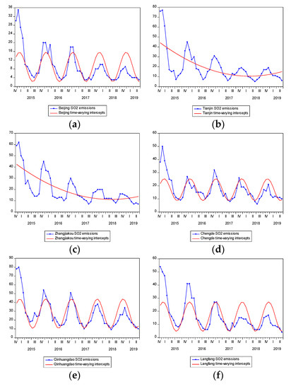
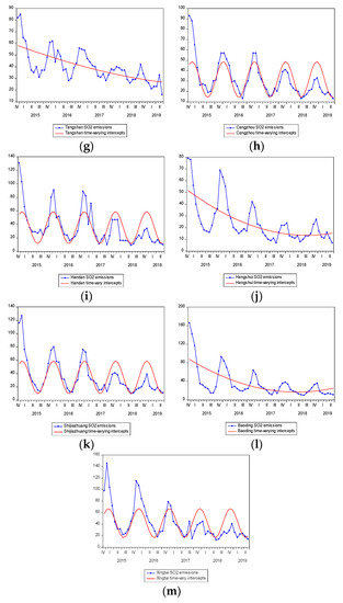
Figure 1.
The Plots of the SO2 emissions per capita and fitted nonlinearities of Beijing-Tianjin-Hebei Urban Agglomeration. (a–m) respectively represent the plots of the SO2 emissions per capita and fitted nonlinearities of Beijing, Tianjin, Zhangjiakou, Chengde, Qinhuangdao, Langfang, Tangshan, Cangzhou, Handan, Hengshui, Shijiazhuang, Baoding, and Xingtai.
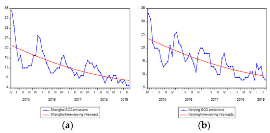
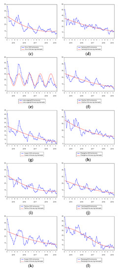
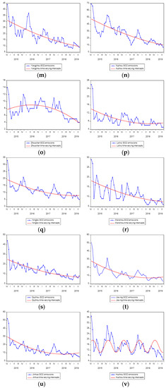
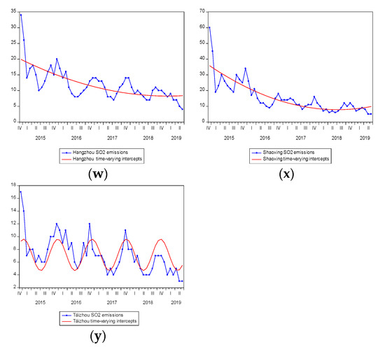
Figure 2.
The plots of the SO2 emissions per capita and fitted nonlinearities of Yangtze River Delta. (a–y) respectively represent the plots of the SO2 emissions per capita and fitted nonlinearities of Shanghai, Nanjing, Wuxi, Nantong, Lianyungang, Suzhou, Huaian, Changzhou, Tàizhou, Yancheng, Suqian, Zhenjiang, Yangzhou, Xuzhou, Zhoushan, Lishui, Ningbo, Wenzhou, Quzhou, Jiaxing, Jinhua, Huzhou, Hangzhou, Shaoxing, and Táizhou.
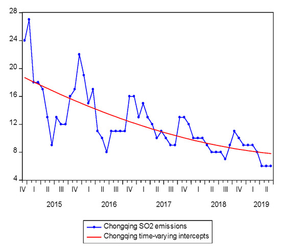
Figure 3.
The plots of the SO2 emissions per capita and fitted nonlinearities of Municipality-Chongqing.
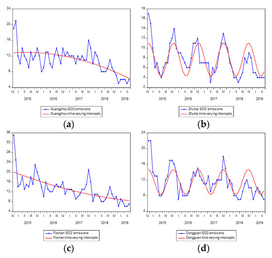
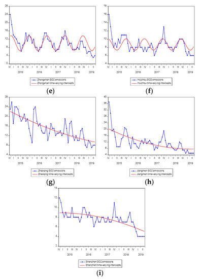
Figure 4.
The plots of the SO2 emissions per capita and fitted nonlinearities of Pearl River Delta. (a–i) respectively represent the plots of the SO2 emissions per capita and fitted nonlinearities of Guangzhou, Zhuhai, Foshan, Dongguan, Zhongshan, Huizhou, Zhaoqing, Jiangmen, and Shenzhen.
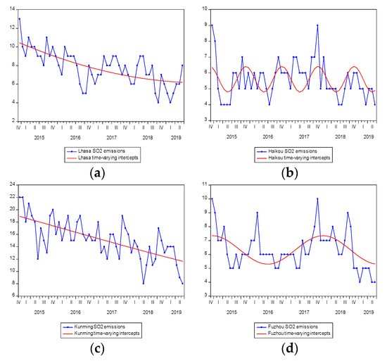
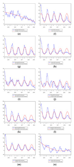
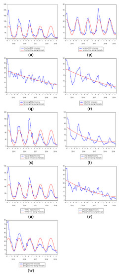
Figure 5.
The plots of the SO2 emissions per capita and fitted nonlinearities of provincial capital cities. (a–w) respectively represent the plots of the SO2 emissions per capita and fitted nonlinearities of Lhasa, Haikou, Kunming, Fuzhou, Chengdu, Xi’an, Guiyang, Urumqi, Nanning, Xining, Shenyang, Changchun, Harbin, Wuhan, Yinchuan, Lanzhou, Nanchang, Hefei, Taiyuan, Ji’nan, Hohhot Changsha, and Zhengzhou.
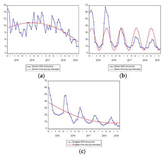
Figure 6.
The plots of the SO2 emissions per capita and fitted nonlinearities of cities under separate state planning. (a–c) respectively represent the plots of the SO2 emissions per capita and fitted nonlinearities of Xiamen, Dalian, and Qingdao.
We first estimate the coefficients of the intercept and autoregressive coefficient , with the corresponding results reported in Table 5. Note that and values are key indicators in determining the permanent/temporary effects of negative and positive shocks, refers to the size of the shocks on each quantile, while plays a crucial role in deciding on the mean reversion of SO2 emissions in each quantile.
Table 5.
Intercept—α0(τ) and autoregressive coefficient—ρ1(τ).
To compare the degree of persistence among quantiles, we plot the aggressive coefficient in Figure 7. In this figure, the solid line represents the values of and dashed line represents a 95% confidence interval. Overall, we observe three types of patterns. First, the values of for SO2 emissions per capita series of Haikou, Shenzhen, Huizhou, Fuzhou, Ningbo, Qingdao, Jiaxing, Jinhua, and Ji’nan display concave or the straight-line upward patterns. The results indicate that the positive shocks to high quantiles of the SO2 emissions per capita of these cities have a more persistent effect than negative shocks to low quantiles, indicating that the positive shocks to the long-run path of the urban–rural income gap will be unbound. The second type pattern can be approximated by the concave or the straight-line download pattern for Suqian and Kunming, which means positive shocks to the SO2 emissions per capita have temporary effects while negative shocks have permanent effects for these two cities. In the third type pattern, the values of for other cities display upward patterns in low quantiles and downward patterns in high quantiles. The results indicate that the high positive and negative shocks to SO2 emissions per capita of these cities have a transitory effect.
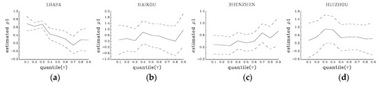
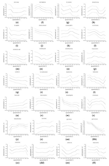
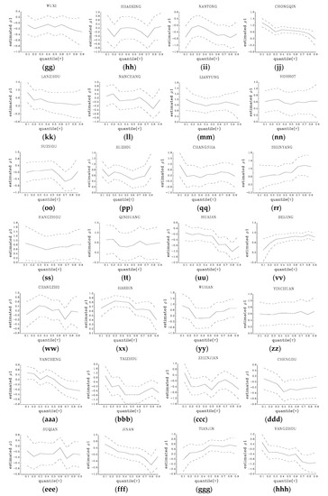
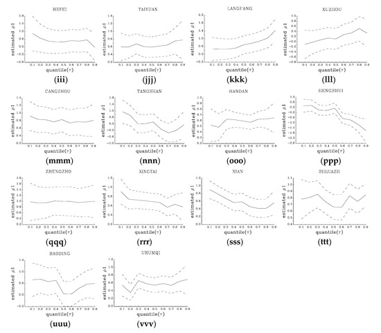
Figure 7.
Autogressive coefficient . (a–vvv) respectively represent the autogressive coefficient of Lhasa, Haikou, Shenzhen, Huizhou, Zhuhai, Kunming, Fuzhou, Zhangjiakou, Xiamen, Zhoushan, Jiangmen, Guiyang, Dongguan, Chengde, Zhongshan, Táizhou, Lishui, Guangzhou, Nanning, Ningbo, Dalian, Wenzhou, Zhaoqing, Foshan, Shanghai, Xining, Quzhou, Qingdao, Jiaxing, Changchun, Jinhua, Nanjing, Wuxi, Shaoxing, Nantong, Chongqing, Lanzhou, Nanchang, Lianyungang, Hohhot, Suzhou, Huzhou, Changsha, Shenyang, Hangzhou, Qinhuangdao, Huaian, Beijing, Changzhou, Harbin, Wuhan, Yinchuan, Yancheng, Tàizhou, Zhenjiang, Chengdu, Suqian, Ji’nan, Tianjin, Yangzhou, Hefei, Taiyuan, Langfang, Xuzhou, Cangzhou, Tangshan, Handan, Hengshui, Zhengzhou, Xingtai, Xi’an, Shijiazhuang, Baoding, and Urumqi.
Table 6 reports , which are used to measure the degree of persistence in each quantile. We can clearly observe that at quantiles between 0.2 and 0.7, the statistic is converging for 62 cities. However, at the extremely low quantile of 0.1, cannot be rejected for Tianjin, Zhangjiakou, Chengde, Tangshan, Xingtai, Shanghai, Nanjing, Lianyungang, Changzhou, Yancheng, Suqian, Yangzhou, Zhuhai, Dongguan, Zhongshan, Zhaoqing, Chongqing, Kunming, Xi’an, Hefei, and Jinan, which means that the SO2 emissions per capita in these 21 cities are divergent when the emissions are high. At the extremely high quantile of 0.9, the SO2 emissions per capita are stationary for 33 cities. These results clearly show that the impact of external changes on SO2 emissions per capita is non-linear and asymmetric and that there is more evidence to support the fact that it is more efficient when using the Fourier function in the model.
Table 6.
Results for Fourier quantile unit root at particular quantiles.
Table 7 reports the results of the unit root hypothesis over the whole quantiles. The optimal frequency and its F statistics are reported at the end of the two columns. The results of Fourier QKS test statistics indicate that the null of unit root over the range of quantiles [0.1, 0.9] is rejected for 13 cities of Beijing–Tianjin–Hebei Urban Agglomeration, 24 cities of Yangtze River Delta, 9 cities of Pearl River Delta, the Chongqing municipality, 22 provincial capital cities, and 3 cities under separate state planning. Only the SO2 emissions per capita of Nanjing and Hefei were not stationary. The optimum frequency varies from 0.1 to 4.8, and the computed F statistics are in all cases greater than the critical values even at 1% significance level, indicating the validity of the choice of the optimal. Hence, the mean-reverting function with the nonlinear component is accepted in favor of the one without the nonlinear component.
Table 7.
Results for overall the Fourier quantile unit root test.
Several important policy implications emerge from our study. First, the convergence of the SO2 emissions per capita for those 72 out of 74 cities does not mean that the environmental improvement goals have been achieved; it only suggests that the past environmental protection work has been effected. More to the point, stationarity indicates that the impact from the SO2 emissions per capita reduction policy is temporary and the SO2 emissions per capita series would revert to a trend path in the long run. Especially for 13 cities in Beijing–Tianjin–Hebei Urban Agglomeration, though the SO2 emissions per capita are converging, the SO2 emission levels are still larger than the levels of the Yangtze River and Pearl River Deltas. Therefore, the policymakers should find more creative and effective ways to curb the SO2 emissions, given that shifting the SO2 emissions from the current level to another would eventually return to its equilibrium level. The environmental situation is not optimistic. A large number of high-pollution industries, such as cement, steel, refining, and petrochemicals, are gathered and the industrial energy consumption is still dominated by coal. Therefore, it is still necessary to actively implement pollution control measures and adjust the structure of industrial sectors.
Second, Nanjing and Hefei are the only two cities where the SO2 emissions per capita are divergent. The environmental protection must be further strengthened because the environmental protection can leave permanent effects. The electricity, heat production and supply industries produce the largest amount of SO2 in these two cities. For a long time, there has been a phenomenon of uncoordinated development of light and heavy industries. The local government should appropriately adjust the industrial structure, increase the proportion of the tertiary industry, and reduce the proportion of the secondary industry, especially the proportion of low-end manufacturing, high-consumption, and high-pollution industries, so that its energy efficiency can be significantly improved and to reduce the SO2 emissions per capita.
Last, our findings suggest that the negative/positive shocks to the SO2 emissions per capita can produce three different effects. Negative shocks to the SO2 emissions per capita in Haikou, Shenzhen, Huizhou, Fuzhou, Ningbo, Qingdao, Jiaxing, Jinhua, and Ji’nan have transitory effects, while positive shocks have permanent effects. On the contrary, positive shocks to the SO2 emissions per capita in Suqian and Kunming have temporary effects, while negative shocks have permanent effects. For the other cities, neither positive nor negative shocks have permanent effects since the SO2 emissions per capita for these cities show stationary behavior. In light of the evidence, local governments should formulate environmental protection policies that are consistent with local practices based on the permanent or transient characteristics of the shocks to the SO2 emissions. This section may be divided by subheadings. It should provide a concise and precise description of the experimental results, their interpretation as well as the experimental conclusions that can be drawn.
4. Conclusions
In this study, we mainly utilized the Fourier quantile unit root test to survey the convergence of the SO2 emissions per capita in 74 cities of China from December 2014 to June 2019, by conducting five traditional unit root tests and a quantile root unit test as a comparative analysis. The empirical results indicate that the SO2 emissions per capita in 72 out of 74 cities in China are converged in the sample period. Only the SO2 emissions per capita in Nanjing and Hefei are divergent. The results also suggest that unit root behavior of the SO2 emissions per capita in these cities is asymmetrically persistent at different quantiles.
Our findings have great implications for the environmental improvement of all cities in China. For the cities with the converging SO2 emissions, the government should consider the asymmetric mean-reverting pattern of SO2 emissions when implementing environmental protection policies at different stages. Moreover, it is worth noting that the environmental protection policies in these cities will not always make a consistent impact on SO2 emissions moving from lower to upper quantiles. For Hefei and Nanjing, the local governments need to enact stricter environmental protection policies to control the emission of sulfur dioxide. In addition, given that the old industrialization route is not desirable, it is thus necessary to implement an energy-saving and material-saving recycling industrial system, which reduces waste discharge per unit of economic output, improves resource utilization efficiency, and achieves low resource consumption and less environmental pollution. Only when the SO2 emissions per capita from cities reach convergence can the SO2 emissions per capita from the country reach convergence.
Author Contributions
Conceptualization, D.-K.S.; methodology, D.-K.S.; formal analysis, B.Z.; data curation, Y.-C.Z.; writing—original draft preparation, D.-K.S. and B.Z.; writing—review and editing, Y.-C.Z. All authors have read and agreed to the published version of the manuscript.
Funding
This research was funded by the National Social Science Foundation of China (Grant number: 18CJY056).
Conflicts of Interest
The authors declare no conflict of interest.
References
- Liu, C.; Hong, T.; Li, H.; Wang, L. From club convergence of per capita industrial pollutant emissions to industrial transfer effects: An empirical study across 285 cities in China. Energy Policy 2018, 121, 300–313. [Google Scholar] [CrossRef]
- Lin, C.; Li, C.; Yang, G.; Mao, I. Association between maternal exposure to elevated ambient sulfur dioxide during pregnancy and term low birth weight. Environ. Res. 2004, 96, 41–50. [Google Scholar] [CrossRef] [PubMed]
- Khan, R.R.; Siddiqui, M. Review on effects of particulates; sulfur dioxide and nitrogen dioxide on human health. Int. Res. J. Environ. Sci. 2014, 3, 70–73. [Google Scholar]
- Goudarzi, G.; Geravandi, S.; Idani, E.; Hosseini, S.A.; Baneshi, M.M.; Yari, A.R.; Vosoughi, M.; Dobaradaran, S.; Shirail, S.; Marzooni, M.B. An evaluation of hospital admission respiratory disease attributed to sulfur dioxide ambient concentration in Ahvaz from 2011 through 2013. Environ. Sci. Pollut. Res. 2016, 23, 22001–22007. [Google Scholar] [CrossRef]
- Wei, J.; Guo, X.; Marinova, D.; Fan, J. Industrial SO2 pollution and agricultural losses in China: Evidence from heavy air polluters. J. Clean. Prod. 2014, 64, 404–413. [Google Scholar] [CrossRef]
- List, J.A. Have air pollutant emissions converged amongst U.S. regions? Evidence from unit-root tests. South. Econ. J. 1999, 66, 144–155. [Google Scholar] [CrossRef]
- Dickey, D.; Fuller, W. Distribution of the estimates for autoregressive time series with unit root. J. Am. Stat. Assoc. 1979, 74, 427–431. [Google Scholar] [CrossRef]
- Mackinnon, J.G. Numerical distribution functions for unit root and cointegration tests. J. Appl. Econom. 1996, 11, 601–618. [Google Scholar] [CrossRef]
- Phillips, P.C.B.; Perron, P. Testing for a unit root in time series regression. Biometrika 1988, 75, 335–346. [Google Scholar] [CrossRef]
- Kwiatkowski, D.; Phillips, P.; Schmidt, P.; Shin, Y. Testing the null hypothesis of stationarity against the alternative of a unit root: How sure are we that economic time series have a unit root? J. Econ. 1992, 54, 159–178. [Google Scholar] [CrossRef]
- Ng, S.; Perron, P. Lag length selection and the construction of unit root tests with good size and power. Econometrica 2001, 69, 1519–1554. [Google Scholar] [CrossRef]
- Strazicich, M.C.; List, J.A. Are CO2 emission levels converging among industrial countries? Environ. Resour. Econ. 2003, 24, 263–271. [Google Scholar] [CrossRef]
- Aldy, J.E. Per capita carbon dioxide emissions: Convergence or divergence? Environ. Resour. Econ. 2006, 33, 533–555. [Google Scholar] [CrossRef]
- Westerlund, J.; Basher, S.A. Testing for convergence in carbon dioxide emissions using a century of panel data. Environ. Resour. Econ. 2008, 40, 109–120. [Google Scholar] [CrossRef]
- Lee, C.C.; Chang, C.P. New evidence on the convergence of per capita carbon dioxide emissions from panel seemingly unrelated regressions augmented Dickey-Fuller tests. Energy 2008, 33, 1468–1475. [Google Scholar] [CrossRef]
- Payne, J.E.; Miller, S.; Lee, J.; Cho, M.H. Convergence of per capita sulphur dioxide emissions across US states. Appl. Econ. 2014, 46, 1202–1211. [Google Scholar] [CrossRef]
- Yavuz, C.N.; Yilanci, V. Convergence in per capita carbon dioxide emissions among g7 countries: A TAR panel unit root approach. Environ. Resour. Econ. 2013, 54, 283–291. [Google Scholar] [CrossRef]
- Li, X.L.; Tang, D.P.; Chang, T. CO2 emissions converge in the 50 US states—Sequential panel selection method. Econ. Model. 2014, 40, 320–333. [Google Scholar] [CrossRef]
- Wu, J.; Wu, Y.; Guo, X.; Cheong, T.S. Convergence of carbon dioxide emissions in Chinese cities: A continuous dynamic distribution approach. Energy Policy 2016, 91, 207–219. [Google Scholar] [CrossRef]
- Herrerias, M.J. CO2 weighted convergence across the EU-25 countries (1920–2007). Appl. Energy 2012, 92, 9–16. [Google Scholar] [CrossRef]
- Burnett, J.W. Club convergence and clustering of the US energy-related CO2 emissions. Resour. Energy Econ. 2016, 46, 62–84. [Google Scholar] [CrossRef]
- Yang, X.; Wang, S.; Zhang, W.; Zhan, D.; Li, J. The impact of anthropogenic emissions and meteorological conditions on the spatial variation of ambient SO2 concentrations: A panel study of 113 Chinese cities. Sci. Total Environ. 2017, 584, 318–328. [Google Scholar] [CrossRef]
- Zhou, Z.; Ye, X.; Ge, X. The impacts of technical progress on sulfur dioxide kuznets curve in China: A spatial panel data approach. Sustainability 2017, 9, 674. [Google Scholar] [CrossRef]
- Yu, S.; Hu, X.; Fan, J.L.; Cheng, J. Convergence of carbon emissions intensity across Chinese industrial sectors. J. Clean. Prod. 2018, 194, 179–192. [Google Scholar] [CrossRef]
- Ulucak, R.; Apergis, N. Does convergence really matter for the environment? An application based on club convergence and on the ecological footprint concept for the EU countries. Environ. Sci. Policy 2018, 80, 21–27. [Google Scholar] [CrossRef]
- Koenker, R.; Xiao, Z. Unit root quantile auto-regression inference. J. Am. Stat. Assoc. 2004, 99, 775–787. [Google Scholar] [CrossRef]
- Perron, P. The great crash, the oil price shock, and the unit root hypothesis. Econometrica 1989, 57, 1361–1401. [Google Scholar] [CrossRef]
- Zivot, E.; Andrews, D.W.K. Further evidence on the great crash, the oil-price shock, and the unit-root hypothesis. J. Bus. Econ. Stat. 1992, 10, 251–270. [Google Scholar] [CrossRef]
- Lee, J.; Strazicich, M.C. Minimum Lagrange multiplier unit root test with two structural breaks. Rev. Econ. Stat. 2003, 85, 1082–1089. [Google Scholar] [CrossRef]
- Lee, J.; Strazicich, M. Minimum LM Unit Root Test with One Structural Break. Econ. Bull. 2013, 33, 2483–2492. [Google Scholar]
- Lee, C.C.; Chang, C.P. Stochastic convergence of per capita carbon dioxide emissions and multiple structural breaks in OECD countries. Econ. Model. 2009, 26, 1375–1381. [Google Scholar] [CrossRef]
- Becker, R.; Enders, W.; Lee, J. A stationarity test in the presence of an unknown number of smooth breaks. J. Time Ser. Anal. 2006, 27, 381–409. [Google Scholar] [CrossRef]
- Christopoulos, D.K.; León-Ledesma, M.A. Smooth breaks and non-linear mean reversion: Post-Bretton-Woods real exchange rates. J. Int. Money Financ. 2010, 29, 1076–1093. [Google Scholar] [CrossRef]
- Lee, J.; Strazicich, M.C.; Meng, M. Two-step LM unit root tests with trend-breaks. J. Stat. Econom. Methods 2012, 1, 81–107. [Google Scholar]
- Meng, M.; Lee, J. More Powerful LM Unit Root Tests with Trend-Breaks in the Presence of Non-Normal Errors; University of Alabama: Tuscaloosa, AL, USA, 2012. [Google Scholar]
- Bahmani-Oskooee, M.; Chang, T.; Elmi, Z.; Ranjbar, O. Re-testing Prebisch-Singer hypothesis: New evidence using Fourier quantile unit root test. Appl. Econ. 2017, 1–14. [Google Scholar] [CrossRef]
- Jarque, C.M.; Bera, A.K. Efficient tests for normality, homoscedasticity and serial independence of regression residuals. Econ. Lett. 1980, 6, 255–259. [Google Scholar] [CrossRef]
© 2020 by the authors. Licensee MDPI, Basel, Switzerland. This article is an open access article distributed under the terms and conditions of the Creative Commons Attribution (CC BY) license (http://creativecommons.org/licenses/by/4.0/).