Abstract
The phenomena of “large energy consumption, high carbon emission, and serious environmental pollution” are against the goals of “low energy consumption, low emissions” in China’s industrial sector. The key to solving the problem lies in improving total factor energy efficiency (TFEE) and carbon emission efficiency (TFCE). Considering the heterogeneity of different sub-industries, this paper proposes a three-stage global meta-frontier slacks-based measure (GMSBM) method for measuring TFEE and TFCE, as well as the technology gap by combining meta-frontier technology with slacks-based measure (SBM) using data envelopment analysis (DEA). DEA can effectively avoid the situation where the technology gap ratio (TGR) is larger than unity. This paper uses the three-stage method to empirically analyze TFEE and TFCE of Anhui’s 38 industrial sub-industries in China from 2012 to 2016. The main findings are as follows: (1) Anhui’s industrial sector has low TFEE and TFCE, which has great potential for improvement. (2) TFEE and TFCE of light industry are lower than those of heavy industry under group-frontier, while they are higher than those of heavy industry under meta-frontier. There is a big gap in TFEE and TFCE among sub-industries of light industry. Narrowing the gap among different sub-industries of light industry is conducive to the overall improvement in TFEE and TFCE. (3) The TGR of light industry is significantly higher than that of heavy industry, indicating that there are sub-industries with the most advanced energy use and carbon emission technologies in light industry. And there is a bigger carbon-emitting technology gap in heavy industry, so it needs to encourage technology spillover from light industry to heavy industry. (4) The total performance loss of industrial sub-industries in Anhui mainly comes from management inefficiency, so it is necessary to improve management and operational ability. Based on the findings, some policy implications are proposed.
1. Introduction
Global warming and other environmental problems caused by excessive energy consumption are becoming more and more serious and have threatened the production and health of human beings [1,2]. Taking environmental issues into account while achieving economic development is becoming a strategy of the state, industries, and even enterprises [3,4]. China, as the world’s most energy-consuming and carbon-emitting country [5], has also set relevant energy-saving and emission-reducing targets. China’s industrial sector, which consumed 68% of its energy in 2015 and emitted 84.2% of its carbon dioxide [6], is the key sector to reduce excessive energy consumption and CO2 emissions by improving total factor energy efficiency (TFEE) and carbon emission efficiency (TFCE) [7,8].
To promote the achievement of energy conservation and emission reduction targets, it is necessary to note that the situation at the national level is not consistent with the situation in a specific province, and different provinces should formulate policies according to their respective factors. Anhui, one of the six central provinces in China and the province that undertakes national industrial transfer, has experienced rapid economic growth in recent years, accounting for 3.3% of total GDP in 2016. At the same time, industry development has brought a continuous increase in industrial energy consumption and carbon emissions. In 2016, industrial energy consumption accounted for 66.87% of the total energy consumption in Anhui. As a key province with the two important national strategies, the analysis of industrial TFEE and TFCE in Anhui plays an important role in accelerating energy-saving and emission reduction and promoting a better realization of the “made in China 2025” target. This paper analyzes the TFEE and TFCE of 38 industrial sub-industries in Anhui.
The main objective of this paper is to explore whether the conclusions of TFEE and TFCE about industrial sub-industries are consistent in both national and provincial perspectives. Under the framework of meta-frontier, we estimate the TFEE, TFCE, and technology gap ratio TGR of industrial sub-industries in Anhui province using the slacks-based measure (SBM) model containing undesirable outputs. Additionally, considering that the meta-frontier slacks-based measure (MSBM) model may measure the TGR greater than 1, this paper proposes a three-stage global meta-frontier slacks-based measure (GMSBM) method based on the MSBM model and the global production technology set. Based on the three-stage GMSBM method, this paper analyzes TFEE and TFCE of 38 industrial sub-industries in Anhui from 2012 to 2016. And we have the following research findings: (1) The overall efficiency level of industrial sub-industries in Anhui is low, with the average TFEE and TFCE under meta-frontier only being 0.1897 and 0.2089, respectively. (2) Although the TFEE and TFCE of light industry are lower than those of the heavy industry under group-frontier, the TFEE of light industry under meta-frontier is higher than that of the heavy industry, showing a trend of decline first and then rise. Moreover, the TFCE under the meta-frontier of light industry is also higher than that of heavy industry. The TFCE of heavy industry declines first and then rises, while the change trend of light industry is not obvious. (3) The TGR of light industry (close to 1) is significantly larger than that of heavy industry, and the carbon emission technology gap of heavy industry is larger than that of the energy technology gap; (4) The total loss of industrial sub-industries in Anhui mainly comes from that caused by management inefficiency.
The remainder of this paper is organized as follows. Section 2 reviews the literature on TFEE and TFCE. Section 3 introduces the methodology in this paper, the proposed three-stage GMSBM model. Section 4 analyzes TFEE and TFCE of light and heavy industries in Anhui and results are discussed in Section 5. Conclusions and policy implications are presented in Section 6.
2. Literature Review
Compared with the traditional single-factor index, such as energy intensity, Zhou et al. [8] put forward TFEE for the first time, including assets and labor force into the framework of energy efficiency measurement. The paper eliminates the substitution relationship between energy and other input indexes under the single factor framework, which makes the energy efficiency measurement system more in line with practical production activities. Based on the original contribution of Hu and Wang [9], a large number of scholars began to use the total factor framework to measure TFEE and TFCE. Accordingly, more and more attention has been paid to the study of TFEE and TFCE in China [10].
2.1. Provincial TFEE or TFCE in China
Some scholars focus on measuring provincial TFEE or TFCE in China. Li and Lin [11] measured the TFEE of 30 provinces from 1997 to 2011 by combining meta-frontier and improved directional distance function (DDF). The results showed that the east of China had the best energy utilization technology, followed by the west, and the central region. And the technology gap is the smallest in the east. Zhang et al. [12] obtained similar results based on MSBM and total factor ecological energy efficiency (ETFEE) analysis of 30 provinces in China from 2001 to 2010. Different from [9,10], Yang et al. [13] measured the TFEE of 30 provinces in China in 2013 and 2014 by using the super-efficient SBM model with unexpected output. The conclusion showed that the TFEE is the highest in the east, but the central region is larger than the western region. Du et al. [14] and Yang and Wang [15] used DDF to calculate the TFCE of various provinces in China. They found that China has a large potential improvement in TFCE, and regional heterogeneity is obvious. Some scholars also studied TFEE and TFCE simultaneously and found that the TFEE and TFCE in China were not high, but the east always performed better [16,17].
2.2. TFEE or TFCE at the National Sectorial Level
Other scholars focused on measuring TFEE or TFCE at the national sectoral level, while the manufacturing sector becomes the key industry to analyze energy consumption and pollution emissions. Li and Lin [18] studied the TFEE improvement potential of 27 manufacturing industries in China from 1998 to 2011. The results showed that the energy types that need to be saved are different among different manufacturing sub-sectors. That is, the energy-saving targets are not the same across industries. Li and Lin [19] examined the eco-energy efficiency performance of light and heavy industries in China from 2003 to 2012, and the results showed that ETFEE of light industry performed better, but the technology of heavy industry was more advanced. Zhang et al. [20] proposed the non-radial global Malmquist carbon emission performance index (NGMCPI) and dynamically measured the TFCE of 38 industrial sectors in China from 1990 to 2012. The results showed that there was a gap among different types of industrial sub-industries for carbon emission performance. And the carbon emission performance of high energy-consuming industries is better. To improve the identification ability and comparability of inter-temporal observations, Zhang et al. [21] proposed the global meta-frontier non-radial directional distance function (GMNDDF) method to measure the carbon emission performance of 28 sub-industries of China’s manufacturing industry from 1990 to 2012. The results showed that there were obvious differences in the carbon emission performance of China’s manufacturing industry. Clearly, the above studies indicate that there are significant differences in TFEE and TFCE between industrial or manufacturing sub-industries.
2.3. TFEE or TFCE at the Provincial Industrial Sector
Some literatures further focused on the whole industrial sector of each province, and this kind of literature is mainly analyzed from the perspective of industry. Feng and Wang [22] analyzed the TFEE and energy-saving potential of 30 provincial-level industrial sectors in China from 2000 to 2014. The results showed that industrial energy efficiency improved greatly during the sample period, but it was still very low. And it argued that eliminating regional imbalances will help improve energy efficiency. Zhao et al. [23] studied the changes in TFEE of industrial sectors of 10 provinces in China from 1997 to 2007 and reached a similar conclusion. Cheng et al. [24] estimated the total-factor carbon emission efficiency index (TCEI) of industrial sectors in 30 Chinese provinces from 2005 to 2015. The results showed that TCEI under meta-frontier (MTCEI) of China’s industrial sectors were very low and have significant spatial heterogeneity. Feng et al. [1] and Zhang et al. [2] analyzed TFCE and emission reduction potential of industrial sectors in 30 Chinese provinces. They found that the TFCE of industrial sectors in all provinces of China is inefficient. And the Chinese government should formulate diversified policies according to the actual situation of different regions. Based on the above studies, there are significant spatial heterogeneity and regional differences in the TFEE and TFCE of China’s industrial sectors. Diversified and targeted policies need to be formulated according to specific conditions of different provinces, with the focus on eliminating efficiency differences between different regions, so as to improve the TFEE and TFCE of China’s industrial sector.
2.4. TFEE or TFCE at the Industrial Sub-Industries
In terms of TFEE and TFCE analysis of industrial sub-industries in specific provinces, [25] calculated the TFEE of 35 industrial sub-industries in Beijing from 2005 to 2012. The results showed that the TFEE of Beijing’s industrial sector is high and on the rise. It also raises the need to strengthen technological innovation and provide policy support to TFEE industries. Fan et al. [26] first studied the dynamic change in total-factor carbon emission performance of 32 industrial sub-industries in Shanghai from 1994 to 2011. The results showed that there was obvious heterogeneity in these 32 sub-industries, and only a few leading industries were in the innovation process, which promoted the improvement in the overall efficiency of the industrial sector in Shanghai. Governments can help companies develop and update green technologies by reducing taxes and increasing environmental regulation. Wu et al. [27] pointed out that national targets should be decomposed into targets at different regional levels, which is more conducive to the effective implementation of energy conservation and emission reduction policies. To achieve the overall national goal of energy saving and emission reduction, it must be implemented at the provincial and municipal level [28]. Therefore, it is helpful to propose policies with more practical significance by refining the research to industrial sectors of provinces.
2.5. Heterogeneity of Production Technology
Due to differences in geographical location, production technology, and economic development, decision-making units (DMUs) are not all in the same production technology set [29]. Disregarding the heterogeneity of different groups will lead to a deviation of the estimated relative efficiency [30,31]. Therefore, the study of TFEE and TFCE in China should consider the heterogeneity of production technology in different regions or industries. O’Donnell et al. [32] proposed the meta-frontier DEA method based on the idea of heterogeneity. Zhang et al. [33] proposed meta-frontier DDF by combining meta-frontier and DDF. Using combination meta-frontier with the DDF or SBM method, regional heterogeneity in eastern, central and western China was considered in existing literatures [11,12,14,16,22,24]. Other literatures considered heterogeneity among different sectors [18,21,34]. Using combination meta-frontier with the traditional DEA model, Zhao et al. [23] considered the heterogeneity from both regional and industrial sectors. Since the implementation of the DDF method requires a given directional vector, different directional vectors may lead to completely different results. Therefore, following Li and Lin [19], this paper studies the TFEE and TFCE of industrial sub-sectors in Anhui based on the MSBM model.
3. Methodology
3.1. The SBM Model
Suppose that there are sub-industries to be estimated, and each sub-industry uses inputs x (capital stock, labor, and energy) to produce the desirable output y (industrial added value, IAV) and undesirable output b (CO2). Then the production possibility set (T) can be expressed as:
where T is generally assumed to satisfy the standard axioms of production theory [35,36]. For instance, T is a closed set, and inactivity can always take place. Finite amounts of inputs can only produce finite amounts of outputs. In addition, x and y are often assumed to be strongly or freely disposable. Meanwhile, we impose weak-disposability and null-jointness assumptions on T (see [6,7] for details).
After the environmental production possible set being defined, we can use the non-parametric DEA method to construct the production possible set. Then, based on [12,19], T with constant return to scale (CRS) can be expressed as follows:
where is the intensity variable for constructing a convex production possible set. M, R, and J are the number of inputs, desirable outputs, and undesirable outputs.
Reference [37] claimed that if there is non-zero slack, the estimation result of the radial measurement method is biased. Tone [38] proposed the SBM method, which is a non-radial measurement method and can measure the slack of inputs and outputs. Zhou et al. [39] expanded the SBM model by adding undesirable outputs. Based on [12,19,40], the SBM model with undesirable outputs can be expressed as follows:
where the subscript o is the DMU to be estimated, , , and denote the input excess, desirable output shortfall, and undesirable output excess of DMUo, respectively.
Model (3) is non-linear, which can be changed into a linear form by Charnes–Cooper transformation [41]:
The invariance of the transformation process implies that . is between 0 and 1. If and only if , and , DMUo is SBM-efficiency. If and , DMUo is TFEE and TFCE, respectively.
3.2. GMSBM Model
The MSBM with undesirable outputs can incorporate heterogeneity among different industries, slacks, and undesirable outputs. Following [12,19], we define two production possibilities: group frontier technology and meta-frontier technology.
Suppose N DMUs can be separated into H subgroups, based on the different production technologies. The number of DMUs in the h-th group is . So . and are defined as h-th group-frontier and meta-frontier production possibility set, respectively. According to [30], .
Similar to Model (2), we can construct a production possible set under meta-frontier. In addition, to improve the discriminating power and make a comparison across different years, we will incorporate a global technology set into technology [12,17,19]. Its form is as follows:
Then the GMSBM model can be solved by the following DEA model:
Model (6) is also non-linear, which can be changed into a linear form by the Charnes–Cooper transformation:
According to [9], the energy efficiency index (EEI) and carbon emission efficiency index (CEI) of industrial sectors i in group h at period t can be defined as the ratio of target energy input to actual energy input, and the ratio of target carbon emission to actual carbon emission:
where, target input (or emission) = actual input (or emission)—slacks. So:
In Model (10), represents the actual energy consumption of the i-th DMU in group h in period t. represents the energy slacks of the i-th DMU in group h in period t, which can be calculated by Models (3) and (4). The elements in Equation (11) have similar meanings. We can find that both GEEI and GCEI are located between 0 and 1. The larger the value is, the better the performance of the DMUo is. And the closer it is to the frontier of the group, the smaller the corresponding slacks are.
Similarly, under the global meta-frontier, total-factor energy efficiency index under meta-frontier (MTEEI) and MTCEI of DMUo can be expressed as:
Both MTEEI and MTCEI are greater than 0 and less than 1. And the bigger the value is, the more efficient it is under the meta-frontier. When the value is 1, the DMUo is considered efficient. Based on [30,31], the efficiency index under the meta-frontier can be decomposed into intra-group efficiency and TGR:
TGR reflects the technology gap between a specific group-frontier and a meta-frontier. As the meta-frontier technology contains the group-frontier technology, the value of TGR is greater than 0 and less than 1. Moreover, a smaller value of TGR represents a greater technology gap between the group- and meta-frontier.
3.3. The Reason for TGR > 1
When using the non-radial distance function to measure the TGR of the meta-frontier model, [42] found that MTCEI was greater than the GTCEI. That is, the non-radial measurement method would lead to the situation of TGR > 1. As a non-radial method, the SBM model still outcomes the TGR larger than 1. Figure 1 illustrates the situation where TGR, measured by MSBM, is greater than 1. Consider the case of two groups, with only one desirable output (industrial added value, Y) and one undesirable output (CO2). K is the DMU under group-frontier. Corresponding to DMU K, the amounts of Y and CO2 are OB and OA, respectively. Moreover, the projection point of K at group-frontier 1 is K1, and the projection point at the meta-frontier is K2. Corresponding to K1, the amounts of Y and CO2 are OD and OC. The Y and CO2 corresponding to K2 are OF and OE. According to Equations (11) and (13), the total-factor carbon emission efficiency index under a specific group-frontier (GTCEI) and MTCEI of DMU K are and , respectively. Then the carbon emission TGR (CTGR) calculated by Equation (15) is . Since OE is greater than OC, the CTGR value is greater than 1.

Figure 1.
Occurrence of the technology gap ratio (TGR) > 1 in the meta-frontier slacks-based measure (MSBM).
3.4. Three-Stage GMSBM Approach
Similar to [42], this paper proposes a three-stage GMSBM model to measure TFEE and TFCE performance and technology gap. The first stage is to calculate GTEEI and GTCEI. Models (3) and (4) can be used to determine the contractions of input and undesirable output and the expansions of expected output. Then we can obtain the projection under the specific group-frontier.
The second stage uses results from the first stage to calculate the TGR. To distinguish TGR of previous literatures, the TGR obtained at this stage is called TGR*. And we can use Equation (16) (this model is similar to the super-efficiency model. Reference [11] mentioned that the value calculated by traditional DEA and super-efficiency DEA is the same for inefficient DMU) to calculate TGR*:
where the values of , , and are the slacks of input, undesirable output, and desirable output, respectively, calculated in the first stage. , and are the slacks of the projection point of DMUo under the specific group-frontier.
Model (16) can be converted to a linear form by the Charnes–Cooper transformation. Based on Model (16), Equations (17) and (18) can be used to measure the heterogeneity between group- and meta-frontier. From the constraints of Model (16), we can know that and , so the values of energy TGR (ETGR) and CTGR are all between 0 and 1.
Similarly, the higher the value of TGR is, the smaller the gap between group- and meta-frontier, i.e., the smaller the technology gap.
The third stage is to use the results from the first and second stages to calculate MTEEI and MTCEI under the meta-frontier. Equations (19) and (20) are the expressions for calculating the efficiency index under the meta-frontier. It is easy to know that these two efficiency indices are between 0 and 1. When the efficiency index is unity, the DMUo is efficient under the meta-frontier. If the efficiency index is less than 1, then the DMU is inefficient.
Figure 2 illustrates the three steps in this paper to calculate the efficiency index under group-frontier, TGR, and meta-frontier. First, K1 is the projection point of K under group1 in the first stage, and , , and are obtained. In the second stage, with the meta-frontier as the reference set, K1 still has room for improvement. And we can obtain the reference point K2’,, , and are the slacks. Then K1K2’ is the technology gap between group-frontier and meta-frontier.
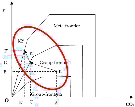
Figure 2.
The three-stage model in this paper.
4. Empirical Analysis
4.1. Data
This paper mainly considered the TFEE and TFCE of Anhui’s industrial sub-industries. The input variables were capital stock, labor, and energy input, the desirable output was IAV, and the undesirable output was CO2. Considering the availability of industry data and the adjustment of industry classification standards in 2011, we collected panel data of 38 industrial sub-industries in Anhui from 2012 to 2016. The labor and IAV can be directly obtained from the Anhui Bureau of Statistics from 2013 to 2017, and the remaining three variables can be calculated by the following methods.
Capital stock (K) can be estimated using the perpetual inventory method [6,20], as follows:
where are capital stock, fixed assets investment, depreciation rate at time t, and the capital stock in period t−1, respectively. The net fixed asset value in 2012, which has been depreciated by the fixed asset price index, was taken as the capital stock in the base period. The specific algorithm depreciation rate and can refer to [6].
Energy input (E) used the amount of raw energy consumed over the years by various industrial sectors, including raw coal, cleaned coal, coke, coke oven gas, crude oil, gasoline, kerosene, diesel, liquefied petroleum gas, natural gas, heat, electricity, and other energy inputs, and all of them were converted into standard coal equivalent (tons).
We follow the guideline provided by IPCC (Intergovernmental Panel on Climate Change) for National Greenhouse Gas Inventories to calculate carbon emissions, and the formula is given as follows:
where , and represents energy consumption, the carbon content factor, the heat equivalent, and the carbon oxidation factor of the carbonaceous fuel i, respectively. The number (44/12) is the ratio of the molecular weight of CO2 (44) to the molecular weight of carbon (12) [7,43]. According to the terminal energy consumption given in the statistical yearbook of Anhui, this paper included the following five energy sources in the calculation of carbon dioxide emissions: raw coal, gasoline, kerosene, diesel, and natural gas. Table 1 is a statistical description of input and output data. It is worth noting that each input and output variable had a large standard deviation, and the range was also substantial, indicating that there was a large difference between different sub-industries. Thus, it is necessary to take heterogeneity into account.

Table 1.
Descriptive statistics of variables in 2012–2016.
4.2. Heterogeneity Across Sub-Industries
As shown by the Chinese National Bureau of Statistics (CNBS), light industry is the sector that mainly provides consumer goods and makes handmade tools, and heavy industry mainly provides the material and technological basis for other sectors of the national economy. Reference [21] also pointed out that a characteristic of heavy industry is that its products are usually intermediate ones for other sub-industries. The products of light industry are used by the ultimate consumer. Therefore, we can divide industrial sub-industries into light and heavy ones to take heterogeneity into consideration. Table A1 shows the details of the classification.
Table 2 is the statistical description of light and heavy industries. It suggests that there is a substantial difference between light and heavy industries in Anhui. Light industry tends to be labor-intensive, while heavy industry tends to be capital-intensive and energy-intensive. The energy intensity and carbon emission intensity of heavy industry are obviously higher. It is reasonable to consider the heterogeneity of heavy and light industries.
Table 2.
Descriptive statistics of light and heavy industries.
4.3. Total-Factor Energy Efficiency Analysis
4.3.1. GTEEI
Table 3 shows the results of GTEEI. For both groups, the average GTEEI of heavy industry was 0.3510, which is relatively high. The GTEEI of manufacture of electrical machinery and apparatus (H17), manufacture of measuring instruments and machinery (H19), and utilization of waste resources (H21) were always unity during the sample period, indicating that their energy-using had always been efficient. Comparing with other heavy sub-industries, other manufacturing (H20) was more efficient. However, the GTEEI of mining and washing of coal (H1), and mining and processing of non-metal Ores (H4), manufacture of raw chemical materials and chemical products (H6), manufacture of non-metallic mineral products (H9), smelting and pressing of ferrous metals (H10), production and supply of electric power and heat power (H23), and production and supply of water (H25) are less than 0.1, which were relative low, and had a large increasing potential.
Table 3.
Average total factor energy efficiency (TFEE) under group- and meta-frontier (2012–2016).
For light industry, the average GTEEI was 0.2841. The GTEEI of manufacture of tobacco (L4) and manufacture of furniture (L9) both reached unity in the past five years, indicating that the TFEE of these two industries, which are the benchmarking for light industry, has always been in the frontier. Comparing with other sub-industries of light industry, the GTEEI of manufacture of foods (L2), manufacture of liquor, beverages and refined tea (L3), manufacture of textile (L5), manufacture of paper and paper products (L10) and manufacture of chemical fibers (L13) were less than 0.1, which performed poorly within their group-frontier.
4.3.2. ETGR*
Figure 3 shows the dynamic trend of average ETGR* for both light and heavy industries. The value of ETGR* of light industry was bigger than that of heavy industry in the sample period. It shows that the energy technology gap of heavy industry was larger than that of light industry. The average ETGR* of heavy industry was 0.1293 to 0.9447, and that of light industry was 0.9677. It implies that if the gap between the two frontiers is eliminated through technology learning and innovation, the level of heavy industry technology can be improved by 5.53%–87.07%, and light industry by 3.23%.

Figure 3.
Dynamic trends of average energy TGR (ETGR*).
As shown in Figure 4, for light industry, manufacture of furniture (L9) had the smallest ETGR*, with a mean value of 0.5028. Among heavy sub-industries, mining and washing of coal (H1), manufacture of non-metallic mineral products (H9), and smelting and pressing of ferrous metals (H10) had the smallest ETGR*, both of which were 0.1293. In addition, there were many heavy sub-industries with relatively low ETGR* and a large technology gap. On the contrary, ETGR* of many light industry sub-sectors was close to unity, indicating that heavy industry can further improve energy utilization technology to improving TFEE in Anhui.
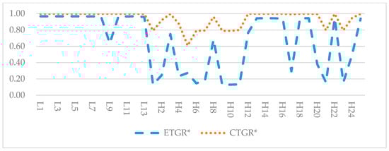
Figure 4.
TGR* at sub-industries level.
4.3.3. MTEEI
MTEEI can be calculated by Equation (19). Table 3 shows the MTEEI values of light and heavy industries. We can conclude that the MTFEE values of both industries were generally low, both showing a trend of decline first and then rise. And the TFEE of light industry was higher than that of heavy industry. Figure 5 shows the box-plot of MTEEI by year by groups. We note that the standard deviation of light industry was greater than that of heavy industry, indicating that there was a large gap in TFEE among sub-industries within the light industry.

Figure 5.
Box-plot of total-factor energy efficiency index under meta-frontier (MTEEI) by year by groups.
The MTEEI of manufacture of tobacco (L4) and manufacture of measuring instruments and machinery (H19) was relatively larger, both of which were 0.9677 and 0.9447, respectively. Production and supply of electric power and heat power (H23) had the lowest MTEEI of 0.0016. Among the 14 industries whose MTEEI were less than 0.1, heavy industry accounted for 10, indicating that the TFEE of the heavy sub-industries was poorer and the energy utilization technology level was relatively low.
4.4. Total-Factor Carbon Emission Performance Analysis
4.4.1. GTCEI
Table 4 shows the results of GTCEI. The average GTCEI for heavy industry was 0.3491. Among them, the GTCEI of manufacture of electrical machinery and apparatus (H17), manufacture of measuring instruments and machinery (H19), and utilization of waste resources (H21) was always unity during the sample period, indicating that the carbon emission performance was efficient. Smelting and pressing of non-ferrous metals (H11) and other manufacturing (H20) were relatively efficient compared with other industries. The GTCEI of mining and washing of coal (H1), manufacture of raw chemical materials and chemical products (H6), manufacture of non-metallic mineral products (H9), manufacture of metal products (H12), manufacture of general-purpose machinery (H13), manufacture of automobiles (H15), repair service of metal products, machinery and equipment (H22), and production and supply of electric power and heat power (H23) were less than 0.1, all of which show relatively poor performance and should take advantage of existing technologies to achieve higher efficiency.
Table 4.
Average total carbon emission efficiency (TFCE) under group- and meta-frontier (2012–2016).
For light industry, the average GTCEI was 0.3132. Manufacture of Tobacco (L4) and manufacture of furniture (L9) always achieved carbon emissions efficient, and the GTCEI remained to be unity. This indicates that the carbon emission performance of these two industries had been on the frontier within the light industry group. Among the other industries, manufacture of textile, wearing apparel, and accessories (L6) performed relatively well, with a GTCEI of 0.6267. The GTCEI of processing of food from agricultural products (L1), manufacture of foods (L2), wine, manufacture of liquor, beverages, and refined tea (L3), manufacture of paper and paper products (L10), and manufacture of chemical fibers (L13) were all less than 0.1, all of which showed relatively poor performance, and should take advantage of existing technologies to achieve group-frontier.
4.4.2. CTGR*
As shown in Figure 6, the CTGR* of heavy industry was smaller than that of light industry, which was the same as the result for ETGR* in Figure 3. The mean values of the CTGR* of heavy industry were from 0.5967 to 0.9520, and those of light industry were from 0.9520 to 0.9565. It indicates that if the gap within two frontiers was eliminated through technological innovation to achieve the meta-frontier, the level of heavy industry technology can be improved by 4.8%–40.33%, and light industry can be improved by 4.35%–4.8%.

Figure 6.
Dynamic trends of average carbon emission TGR (CTGR*).
As shown in Figure 4, the ETGR* of light industry was higher, and the carbon emission technology gap was relatively small. Among light sub-industries, manufacture of furniture (L9) had the highest CTGR* value, and its carbon emission technology was better. The remaining sub-industries were 0.9520. Among heavy sub-industries, the values of CTGR* of utilization of waste resources (H21) and production and supply of electric power and heat power (H23) were the smallest, which was 0.5967. Manufacture of metal products (H12), manufacture of general-purpose machinery (H13), and production and supply of water (H25) had the largest CTGR* with 0.9520.
4.4.3. MTCEI
Table 4 lists the values of MTCEI for light and heavy industries. Similar to the results of MTEEI, the mean value of MTCEI for light industry was significantly larger than that for heavy industry, which were 0.2985 and 0.1623, respectively. MTCEI of heavy industry showed the trend of first decline and then rise, while the change trend of light industry was not obvious. Figure 7 shows the box-plot of MTCEI by year by groups. We note that standard deviations for light industry were higher, suggesting that there was a large gap for TFCE of sub-industries across light industry.

Figure 7.
Box-plot of meta-frontier total-factor carbon emission efficiency index (MTCEI) by year by groups.
For the sub-industries level, consistent with MTEEI’s conclusion, production and supply of electric power and heat power (H23) had the worst performance, with an MTCEI of just 0.0007. Manufacture of furniture (L9) achieved the meta-frontier as its MTCEI remained 0.9565. There were 20 sub-industries that MTCEI was less than 0.01, among which 15 were within heavy industry, indicating that heavy sub-industries showed relatively poor carbon emission performance under the meta-frontier.
4.5. The Decomposition of Total Performance Loss
According to the above efficiency analysis of group-frontier and meta-frontier, we can get two target energy/carbon intensities: GEI/GCI and MEI/MCI. GEI/GCI represents the energy/carbon intensity of a projection point under the group-frontier for a sub-industry. MEI/MCI is the energy/carbon intensity value for the projection point on the meta-frontier. By comparing the actual energy/carbon intensity (AEI/ACI) with the target energy/carbon intensity, we can decompose the total performance loss (TPL) into the loss caused by management inefficiency (MIL) and the loss caused by technology gap (TGL). TPL of energy (ETPL) can be expressed by Equations (23)—(25) (TPL of carbon emissions (CTPL) has similar expression):
Figure 8 and Figure 9 describe the average values of the two industrial groups and all industrial sectors during the sample period for sources of TFEE and TFCE losses in light and heavy industries. Overall, ETPL and CTPL accounted for 89.2% and 99.5% of management factors, respectively. As mentioned above, light industry is the main benchmark for meta-frontier, so the loss caused by its technical factors was very low. Compared with CTPL, ETPL had more performance loss due to MIL.

Figure 8.
Sources of energy total performance loss (ETPL) in two industrial groups.

Figure 9.
Sources of carbon emissions TPL (CTPL) in two industrial groups.
Figure 10 and Figure 11 describe the sources of performance losses at the sub-industry level during the sample period. The ETPL of manufacture of tobacco (L4), manufacture of furniture (L9), manufacture of electrical machinery and apparatus (H17), manufacture of measuring instruments and machinery (H19), and utilization of waste resources (H21) and the CTPL of manufacture of tobacco (L4), manufacture of furniture (L9), smelting and pressing of non-ferrous metals (H11), manufacture of electrical machinery and apparatus (H17), manufacture of measuring instruments and machinery (H19), and utilization of waste resources (H21) were derived from technological factors. Therefore, these sub-industries need to improve energy utilization and carbon emission technologies. Other sub-industries should focus on management factors to improve performance.
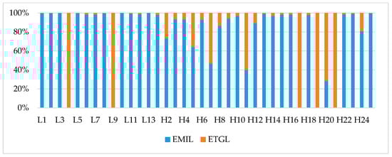
Figure 10.
Sources of ETPL among sub-industries.
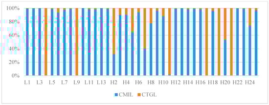
Figure 11.
Sources of CTPL among sub-industries.
5. Discussion
Based on the empirical results, it can be seen that, in general, the overall TFEE and TFCE of the industry sector in Anhui province were relatively low, and there was a big gap among the sub-industries. Lower TFEE and TFCE averages in light industry under group-frontier indicate a bigger gap among sub-industries and a more uneven development of light industry. For TGR*, the ETGR* and CTGR* of light industry were both larger, indicating that the corresponding technology of light industry in Anhui province was more advanced. Light industry tends to be labor-intensive rather than technology-intensive, so it is generally assumed that the technology of light industry will be more advanced, but efficiency analysis takes into account the entire production process, so the more advanced technology here is energy-use technology and carbon-emission technology that take into account the elements of inputs and outputs. These two main findings differ from those at the national level that Li and Lin [19] found that at the national level light industry had higher intra-group efficiencies and more advanced technology than heavy industry. Under meta-frontier, light industry in Anhui province had more TFEE and TFCE than heavy industry. This conclusion is consistent with that at the national level.
At the individual industries level, under group-frontier, manufacture of tobacco (L4), manufacture of furniture (L9), electrical machinery and apparatus (H17), manufacture of measuring instruments and machinery (H19) and utilization of waste resources (H21) all achieved energy efficiency within their respective groups, whose GTFEE were 1. Manufacture of electrical machinery and apparatus (H17), manufacture of measuring instruments and machinery (H19), utilization of waste resources (H21), manufacture of Tobacco (L4), and manufacture of furniture (L9) achieved carbon emission efficiency within their respective groups, whose GTCEI were 1. These industries were at the frontier of each group, making better use of existing technology within the group.
Under meta-frontier, whether for MTEEI or MTCEI, more sub-industries under heavy industry performed poorly during the study period. Production and supply of electric power and heat power (H23) had the worst MTEEI and MTCEI. But it should be noted that the increase in heavy industry was more obvious.
The total performance loss (TPL) of mining and processing of non-metal ores (L4), manufacture of non-metallic mineral products (L9), manufacture of non-metallic mineral products (H7), smelting and pressing of non-ferrous metals (H11), manufacture of measuring instruments and machinery (H19) and utilization of waste resources (H21) was more or all derived from the technology gap, while TPL of other sub-industries was more derived from the management ineffectiveness. This also requires industry-wide regulatory strengthening to reduce ETPL and CTPL.
Anhui Province implemented a light industry strong provincial strategy in 2009. In the early stage of development, priority should be given to the development of several specific industries of light industry to promote the overall development, which may lead to the rapid development of light industry than heavy industry, and the development gap between sub-industries within light industry is larger. Therefore, for the industry of Anhui Province, to better develop industry, we should narrow the gap of light industry and balance the development between industries. Emphasis should also be placed on technological innovation and progress in heavy industry, especially technologies related to energy use and carbon emissions.
6. Conclusions and Policy Implications
For China’s TFEE and TFCE, existing literature has conducted fruitful research on national, provincial, and industrial levels, respectively. Research at the national level takes into account the country as a whole, but there are often differences among provinces. Exploring whether a conclusion province’s perspective is the same as a country’s is an important starting point. Meanwhile, the distinguishing feature of “high energy consumption and high carbon emission” in the industrial sector makes TFEE and TFCE become the focus of scholars. In view of this, considering the heterogeneity among different sub-industries, this paper proposed a three-stage GMSBM method to circumvent the situation where the TGR was greater than 1 and analyzed the TFEE and TFCE of industrial sub-industries in Anhui, one of China’s six central provinces.
The main findings in this paper are summarized as follows. First, the TFEE and TFCE of light and heavy industries were low under group-frontier and meta-frontier. Therefore, there is great potential for improvement. Second, under group-frontier, the TFEE and TFCE of light industry were lower than those of heavy industry, while under meta-frontier, the TFEE and TFCE of light industry were higher than those of heavy industry. It indicates that there is a big gap between sub-industries within light industry group. Narrowing the gap between different light sub-industries is conducive to the overall improvement in TFEE and TFCE. Third, TGR* was higher in light sub-industries than in heavy ones, indicating a smaller technology gap in light industries. Moreover, compared with the energy technology gap, the carbon emission technology gap of heavy industry was larger. Fourth, from the perspective of the sources of TPL, most sub-industries need to reduce the performance loss caused by management factors.
Based on the above findings, we put forward some policy implications. First, the provincial government in Anhui needs to formulate strict environmental protection policies to stimulate industrial enterprises to improve the performance of energy utilization and carbon emission. Meanwhile, exchanges and learning of energy saving and emission reduction technologies should be strengthened among different industrial enterprises to release the potential of energy saving and emission reduction, especially for the light sub-industries with low efficiency under group-frontier, such as manufacture of foods (L2), manufacture of liquor, beverages and refined tea (L3), manufacture of textile (L5), and manufacture of chemical fibers (L13). Second, give full play to the advantages of Hefei (the capital of Anhui) as a scientific and technological innovation city, to improve the energy saving and emission reduction technologies of enterprises. Heavy industry has a large gap in carbon emissions and is the key industry in the study and innovation of emission reduction technology. Within the heavy industry, mining and washing of coal (H1), mining and processing of non-metal ores (H4), manufacture of raw chemical materials and chemical products (H6), manufacture of medicines (H7), manufacture of rubber and plastics products (H8), manufacture of non-metallic mineral products (H9), smelting and pressing of ferrous metals (H10), smelting and pressing of non-ferrous metals (H11), and production and supply of electric power and heat power (H23) are the key sub-industries to narrow technology gap. Third, improving energy structure and increasing the proportion of clean energy use. The energy structure of industrial sectors in Anhui is mainly based on fossil fuels, which will produce a large amount of greenhouse gases. In particular, for the heavy industry sector, its AEI and ACI were very high. Therefore, the improvement of energy structure will play an important role in the energy saving and emission reduction of the heavy industry and the industrial sectors in Anhui. Fourth, MIL was a major source of ETPL and CTPL. Manufacture of tobacco (L4), manufacture of furniture (L9), manufacture of electrical machinery and apparatus (H17), manufacture of measuring instruments and machinery (H19), other manufacture (H20,) and utilization of waste resources (H21) need to be placed on reducing the energy technology gap, while manufacture of tobacco (L4), manufacture of furniture (L9), mining and processing of ferrous metal ores (H2), manufacture of medicines (H7), smelting and pressing of non-ferrous metals (H11), manufacture of electrical machinery and apparatus(H17), manufacture of measuring instruments and machinery (H19), and utilization of waste resources (H21) need to concentrate on reducing the carbon emission technology gap. The remaining sub-industries shall achieve the requirements of energy saving and emission reduction by strengthening and optimizing management practices.
In the future, additional data should be concluded to expand the research of this paper. First, we intend to conclude the emission data of SO2 and COD to calculate the energy efficiency score more accurately. Second, considering the differences among different provinces, this method can be used to further analyze the TFEE and TFCE of other high-emission and high-pollution provinces (such as Hebei) in the future. Naturally, the method proposed in this paper can also be used to evaluate the TFEE and TFCE of other countries or regions. Considering that the period of this paper is not long; this paper only focuses on TFEE and TFCE analysis. If the sample period is longer, the method in this paper also can be extended to further analyze the dynamic changes in TFEE and TFCE.
Author Contributions
Conceptualization, Y.C.; methodology, Y.C., W.X.; software, W.X.; validation, Y.C., Q.Z., Z.Z.; formal analysis, W.X.; investigation, Y.C., W.X., Z.Z; resources, Y.C.; data curation, W.X.; writing—original draft preparation, W.X., Q.Z.; writing—review and editing, Y.C., Q.Z., Z.Z.; visualization, W.X.; supervision, Y.C., Q.Z., Z.Z.; project administration, Y.C.; funding acquisition, Y.C., Z.Z., Q.Z. All authors have read and agreed to the published version of the manuscript.
Funding
This work was supported by National Natural Science Foundation of China (grant numbers 71601064, 71471053, 71871081, 71701059), Major Program of National Fund of Philosophy and Social Science of China (grant number 18ZDA064) and the Fundamental Research Funds for the Central Universities (grant number JZ2017HGTB0184, JZ2019HGTB0095).
Conflicts of Interest
The authors declare no conflict of interest.
Appendix A
Table A1.
Two-digit sub-industries and their classification according to CNBS.
Table A1.
Two-digit sub-industries and their classification according to CNBS.
| Light Industry |
| Processing of food from agricultural products (L1); Manufacture of foods (L2); Manufacture of liquor, beverages and refined tea (L3); Manufacture of tobacco (L4); Manufacture of textile (L5); Manufacture of textile, wearing apparel and accessories (L6); Manufacture of leather, fur, feather and related products and footwear (L7); Processing of timber, manufacture of wood (L8); Manufacture of furniture (L9); Manufacture of paper and paper products (L10); Printing and reproduction of recording media (L11); Manufacture of articles for culture, education, arts and crafts, sports and entertainment activities (L12); Manufacture of chemical fibers (L13); |
| Heavy Industry |
| Mining and washing of coal (H1); Mining and processing of ferrous metal ores (H2); Mining and processing of non-ferrous metal ores (H3); Mining and processing of non-metal ores (H4); Processing of petroleum, coking and processing of nuclear fuel (H5); Manufacture of raw chemical materials and chemical products (H6); Manufacture of medicines (H7); Manufacture of rubber and plastics products (H8); Manufacture of non-metallic mineral products (H9); Smelting and pressing of ferrous metals (H10); Smelting and pressing of non-ferrous metals (H11); Manufacture of metal products (H12); Manufacture of general purpose machinery (H13); Manufacture of special purpose machinery(H14); Manufacture of automobiles (H15); Manufacture of railway, ship, aerospace and other transport equipment (H16); Manufacture of electrical machinery and apparatus (H17); Manufacture of computers, communication and other electronic equipment (H18); Manufacture of measuring instruments and machinery (H19); Other manufacture (H20); Utilization of waste resources (H21); Repair service of metal products, machinery and equipment (H22); Production and supply of electric power and heat power (H23); Production and supply of gas (H24); Production and supply of water (H25); |
Note: “L” means light industry and “H” means heavy industry.
References
- Feng, C.; Zhang, H.; Huang, J.B. The approach to realizing the potential of emissions reduction in China: An implication from data envelopment analysis. Renew. Sustain. Energy Rev. 2017, 71, 859–872. [Google Scholar] [CrossRef]
- Zhang, Y.J.; Hao, J.F.; Song, J. The CO2 emission efficiency, reduction potential and spatial clustering in China’s industry: Evidence from the regional level. Appl. Energy 2016, 174, 213–223. [Google Scholar] [CrossRef]
- Barba-Sanchez, V.; Atienza-Sahuquillo, C. Environmental Proactivity and Environmental and Economic Performance: Evidence from the Winery Sector. Sustainability 2016, 8, 1014. [Google Scholar] [CrossRef]
- Junquera, B.; Barba-Sanchez, V. Environmental Proactivity and Firms’ Performance: Mediation Effect of Competitive Advantages in Spanish Wineries. Sustainability 2018, 10, 2155. [Google Scholar] [CrossRef]
- British Petroleum (BP). BP Statistical Review of World Energy 2017 Workbook; British Petroleum: London, UK, 2017. [Google Scholar]
- Chen, S. Reconstruction of sub-industrial statistical in China (1980–2008). China Econ. Q. 2011, 10, 735–776. (In Chinese) [Google Scholar]
- Zhang, N.; Choi, Y. Environmental energy efficiency of China’s regional economies: A non-oriented slacks-based measure analysis. Soc. Sci. J. 2013, 50, 225–234. [Google Scholar] [CrossRef]
- Zhou, P.; Ang, B.W.; Zhou, D.Q. Measuring economy-wide energy efficiency performance: A parametric frontier approach. Appl. Energy 2012, 90, 196–200. [Google Scholar] [CrossRef]
- Hu, J.L.; Wang, S.C. Total-factor energy efficiency of regions in China. Energy Policy 2006, 34, 3206–3217. [Google Scholar] [CrossRef]
- Meng, F.; Su, B.; Thomson, E.; Zhou, D.; Zhou, P. Measuring China’s regional energy and carbon emission efficiency with DEA models: A survey. Appl. Energy 2016, 183, 1–21. [Google Scholar] [CrossRef]
- Li, K.; Lin, B. Metafroniter energy efficiency with CO2 emissions and its convergence analysis for China. Energy Econ. 2015, 48, 230–241. [Google Scholar] [CrossRef]
- Zhang, N.; Kong, F.; Yu, Y. Measuring ecological total-factor energy efficiency incorporating regional heterogeneities in China. Ecol. Indic. 2015, 51, 165–172. [Google Scholar] [CrossRef]
- Yang, T.; Chen, W.; Zhou, K.; Ren, M. Regional energy efficiency evaluation in China: A super efficiency slack-based measure model with undesirable outputs. J. Clean Prod. 2018, 198, 859–866. [Google Scholar] [CrossRef]
- Du, K.; Lu, H.; Yu, K. Sources of the potential CO2 emission reduction in China: A nonparametric metafrontier approach. Appl. Energy 2014, 115, 491–501. [Google Scholar] [CrossRef]
- Yang, L.; Wang, K.L. Regional differences of environmental efficiency of China’s energy utilization and environmental regulation cost based on provincial panel data and DEA method. Math. Comput. Model. 2013, 58, 1074–1083. [Google Scholar] [CrossRef]
- Yao, X.; Zhou, H.; Zhang, A.; Li, A. Regional energy efficiency, carbon emission performance and technology gaps in China: A meta-frontier non-radial directional distance function analysis. Energy Policy 2015, 84, 142–154. [Google Scholar] [CrossRef]
- Lin, B.; Du, K. Energy and CO2 emissions performance in China’s regional economies: Do market-oriented reforms matter? Energy Policy 2015, 78, 113–124. [Google Scholar] [CrossRef]
- Li, K.; Lin, B. The efficiency improvement potential for coal, oil and electricity in China’s manufacturing sectors. Energy 2015, 86, 403–413. [Google Scholar] [CrossRef]
- Li, J.; Lin, B. Ecological total-factor energy efficiency of China’s heavy and light industries: Which performs better? Renew. Sustain. Energy Rev. 2017, 72, 83–94. [Google Scholar] [CrossRef]
- Zhang, N.; Wang, B.; Liu, Z. Carbon emissions dynamics, efficiency gains, and technological innovation in China’s industrial sectors. Energy 2016, 99, 10–19. [Google Scholar] [CrossRef]
- Zhang, N.; Wang, B.; Chen, Z. Carbon emissions reductions and technology gaps in the world’s factory, 1990–2012. Energy Policy 2016, 91, 28–37. [Google Scholar] [CrossRef]
- Feng, C.; Wang, M. Analysis of energy efficiency and energy savings potential in China’s provincial industrial sectors. J. Clean. Prod. 2017, 164, 1531–1541. [Google Scholar] [CrossRef]
- Zhao, X.; Rui, Y.; Qian, M. China’s total factor energy efficiency of provincial industrial sectors. Energy 2014, 65, 52–61. [Google Scholar]
- Cheng, Z.; Li, L.; Liu, J.; Zhang, H. Total-factor carbon emission efficiency of China’s provincial industrial sector and its dynamic evolution. Renew. Sustain. Energy Rev. 2018, 94, 330–339. [Google Scholar] [CrossRef]
- Wang, J.M.; Shi, Y.F.; Zhang, J. Energy efficiency and influencing factors analysis on Beijing industrial sectors. J. Clean. Prod. 2017, 167, 653–664. [Google Scholar] [CrossRef]
- Fan, M.; Shao, S.; Yang, L. Combining global Malmquist-Luenberger index and generalized method of moments to investigate industrial total factor CO2 emission performance: A case of Shanghai (China). Energy Policy 2015, 79, 189–201. [Google Scholar] [CrossRef]
- Wu, J.; Zhu, Q.; Liang, L. CO2 emissions and energy intensity reduction allocation over provincial industrial sectors in China. Appl. Energy 2016, 166, 282–291. [Google Scholar] [CrossRef]
- Wang, Q.; Su, B.; Sun, J.; Zhou, P.; Zhou, D. Measurement and decomposition of energy-saving and emissions reduction performance in Chinese cities. Appl. Energy 2015, 151, 85–92. [Google Scholar] [CrossRef]
- Hayami, Y.; Ruttan, V. Agricultural development: An international perspective. J. Econ. Hist. 1973, 33, 484–487. [Google Scholar]
- Battese, G.E.; Prasada Rao, D.S.; O’Donnell, C.J. A metafrontier production function for estimation of technical efficiencies and technology gaps for firms operating under different technologies. J. Product. Anal. 2004, 21, 91–103. [Google Scholar] [CrossRef]
- Ding, T.; Wu, H.Q.; Jia, J.J.; Wei, Y.Q.; Liang, L. Regional assessment of water-energy nexus in China’s industrial sector: An interactive meta-frontier DEA approach. J. Clean Prod. 2020, 244, 118979. [Google Scholar] [CrossRef]
- O’Donnell, C.J.; Rao, D.S.P.; Battese, G.E. Metafrontier frameworks for the study of firm-level efficiencies and technology ratios. Empir. Econ. 2008, 34, 231–255. [Google Scholar] [CrossRef]
- Zhang, N.; Zhou, P.; Choi, Y. Energy efficiency, CO2 emission performance and technology gaps in fossil fuel electricity generation in Korea: A meta-frontier non-radial directional distance function analysis. Energy Policy 2013, 56, 653–662. [Google Scholar] [CrossRef]
- Wang, H.; Ang, B.W.; Wang, Q.W.; Zhou, P. Measuring energy performance with sectoral heterogeneity: A non-parametric frontier approach. Energy Econ. 2017, 62, 70–78. [Google Scholar] [CrossRef]
- Färe, R.; Primont, D. Multi-Output Production and Duality: Theory and Applications; Springer: Dordrecht, The Netherlands, 1995; Volume 13, pp. 317–332. [Google Scholar]
- Faere, R.; Grosskopf, S.; Lovell, C.A.K.; Pasurka, C. Multilateral Productivity Comparisons When Some Outputs are Undesirable: A Nonparametric Approach. Rev. Econ. Stat. 2006, 71, 90. [Google Scholar] [CrossRef]
- Fukuyama, H.; Weber, W.L. A directional slacks-based measure of technical inefficiency. SocioEcon. Plann. Sci. 2009, 43, 274–287. [Google Scholar] [CrossRef]
- Tone, K. Theory and Methodology A slacks-based measure of efficiency in data envelopment analysis. Eur. J. Oper. Res. 2001, 130, 498–509. [Google Scholar] [CrossRef]
- Zhou, P.; Ang, B.W.; Poh, K.L. Slacks-based efficiency measures for modeling environmental performance. Ecol. Econ. 2006, 60, 111–118. [Google Scholar] [CrossRef]
- Cooper, W.W.; Seiford, L.M.; Tone, K. Data Envelopment Analysis: A Com-Prehensive Text with Models, Applications, References and DEA-Solver Software, 2nd ed.; Kluwer Academic Publishers: Boston, MA, USA, 2007. [Google Scholar]
- Charnes, A.; Cooper, W. Programming with linear fractional functions. Nav. Res. Logist. Q. 1962, 9, 181–186. [Google Scholar] [CrossRef]
- Wang, Q.; Su, B.; Zhou, P.; Chiu, C.R. Measuring total-factor CO2 emission performance and technology gaps using a non-radial directional distance function: A modified approach. Energy Econ. 2016, 56, 475–482. [Google Scholar] [CrossRef]
- Chang, Y.T.; Zhang, N.; Danao, D.; Zhang, N. Environmental efficiency analysis of transportation system in China: A non-radial DEA approach. Energy Policy 2013, 58, 277–283. [Google Scholar] [CrossRef]
© 2020 by the authors. Licensee MDPI, Basel, Switzerland. This article is an open access article distributed under the terms and conditions of the Creative Commons Attribution (CC BY) license (http://creativecommons.org/licenses/by/4.0/).