Optimize the Banker’s Multi-Stage Decision-Making and the Mechanism of Pay Contract Influencing on Bank Default Risk in the Long-Term Model


1
School of Management, Harbin Institute of Technology, Harbin 150000, China
2
School of Business, Singapore University of Social Sciences, Singapore 599494, Singapore
*
Author to whom correspondence should be addressed.
Sustainability 2020, 12(4), 1400; https://doi.org/10.3390/su12041400
Submission received: 20 January 2020
/
Revised: 5 February 2020
/
Accepted: 10 February 2020
/
Published: 14 February 2020
(This article belongs to the Special Issue Sustainable Banking: Issues and Challenges)
Abstract
:In recent years, researchers have been devoted to illustrating the correlation between bankers’ pay contracts and a bank’s risk-taking behavior where corporate governance is concerned, especially throughout the past four decades and by using empirical analysis. Despite being a widespread concern, the causality of this relationship is not thoroughly understood. We initiate this research by modeling bankers’ multi-stage decisions of option investment and bond investment from the perspective of theoretical analysis, and by analyzing the function image results using data from Wells Fargo & Co. from the ExecuComp, BvD Orbis, and CRSP-COMPUSTAT databases. We aim to deeply explore the mechanism of how compensation influencing on risk. We are the first to find that it has a “risk cap”, which is the optimal risk level to maximize the return of decision-making. We are also the first to discover the optimal decision coefficient level to maximize the decision return, during which the internal causes and mechanisms of the impact of bankers’ compensation on a bank’s default risk are revealed. We also illustrate the influence of the number of periods. We expect our findings to provide advice for establishing policies when designing pay contracts.
1. Introduction
1.1. Research Background and Framework Diagram
In 1976, Jensen and Meckling [1] first published their paper regarding executive compensation, which belongs to the field of corporate governance. Since then, this field has become an object of increasing concern for related scholars. Furthermore, after the financial depression of 2007–2009, researchers realized that banks have unique features different from other non-financial institutions, which could lead to the systematic risk of the whole economic system, even cross-nationally, when the risk level is high or bankruptcy occurs. However, the way in which the pay contracts of bankers influence a bank’s risk-taking behavior or, in other words, the mechanism behind the influence of pay contracts on a bank’s default risk in the long term is still not thoroughly understood.
Figure 1 outlines a schematic diagram of the effect of the decision-making of bankers on the relationship between compensation and the default risk of banks. As is shown in Figure 1, we divide the total compensation into two parts, that is, inside equity and inside debt. Inside equity refers to equity-based compensation, for instance, restricted stock, stock options, and other instruments, of which the value lies in the equity returns in the future. Meanwhile, inside debt is defined as the sum of benefit pensions and deferred compensation, as per Jensen and Meckling [1]. The multi-stage decision-making of a CEO contains the decisions of option investment and bond investment for some times (or in multiple stages) in this paper. The objective of a banker is to maximize the decision return when making decisions. According to the different proportions of option investment and bond investment in the total decision-making process, and the variance of default risk level, the return of executives varies. This, in turn, affects the compensation levels and the structure of pay contracts. The aim of this paper is to determine the optimal level of the default risk and decision weight level (invest more option or bond) in order to find out the deeper mechanism regarding how compensation influences the risk levels of banks—namely, through the decisions of bankers.
1.2. Related Studies
Many researchers have studied structure design from the following perspectives. From the empirical works of their predecessors, Wang and Lin (2009) [2] revealed that risk management can be taken into consideration to select a strategy for the Bank of Kaohsiung. Riachi et al. (2013) [3] examined the effect of corporate asset-backed securitization on managerial compensation. Li et al. (2011) [4] investigated the relationship between stock mispricing, the investment of the firm, and the compensation of bankers from an empirical perspective. Latham and Braun (2010) [5] indicated that there is a positive relationship between corporate debt level and the decision of an IPO (Initial Public Offering). Kokkinis (2019) [6] explored the impacts of the rule of a bonus cap on managers’ decision incentives, which is linked to different degrees of risk. Kim (2015) [7] found that, as the compensation for executives increases, the greater both the investment in R&D (research and development) and the profits become. Kang et al. (2006) [8] implied that executive incentive compensation is endogenously determined, as are the corporate investment policies. Huang et al. (2012) [9] discussed, in detail, the results of the specific interactions between investment and financing decisions. Ho et al. (2016) [10] offered CEO overconfidence as an explanation for the cross-sectional heterogeneity in a bank’s risk-taking behavior. Gulati and Yasin (1994) [11] presented the application of an expert system to time the market right.
On a theoretical level, Grundy and Li (2010) [12] developed a model that is able to predict the increase of corporate investment levels. Eisdorfer et al. (2013) [13] examined the factors that affect the quality of the investment decisions of the corporation. Eastburn and Boland (2015) [14] revealed that bankers narrow the focus of their concentration due to the complexity of their decisions. Bliss and Rosen (2001) [15] examined the relationship between mergers and CEO compensation during 1986 to 1995.
From the perspective of the relationship of bank risk and compensation, Belkhir and Boubaker (2013) [16] showed that CEO inside debt holdings yield a positive influence on hedging. Li et al. [17] provided an advanced inside debt metric superior to the previously used ones. Li and Zhang [18] highlighted the positive relationship between the proportion of female directors and short-maturity debt. Li et al. [19] found that the greater the amount of inside debt that a CEO holds, the lower the possibility to issue convertibles rather than straight debt by firms. Merton (1974) [20] used a framework to design the compensation of bankers based on the concept of the European call option of Black and Scholes.
In addition to the abovementioned research, our study provides significant insight to better understand the stability of banks or other financial institutions. Just as Abad-Segura et al. [21] wrote, companies should be obliged to work toward social responsibility by using a sustainability approach, including banks.
Overall, there are limited studies regarding the mechanism behind the influence of compensation on risk, especially on a theoretical level. Thus, attempting to uncover this mechanism on a theoretical level is also a particular aim of our research.
1.3. Research Progress
In this article, we initiate this research by setting up a multi-stage decision-making model, containing both option investment and bond investment, to deeply explore the mechanism of how compensation influencing on risk, based on our previous work (Ma et al., 2020 [22,23]) on a banker’s long-term compensation and the design of pay contracts. We demonstrate the relationship between the decision return of multi-stages and both the risk and the decision weight of the bank by developing a particular formula. After setting up this model, we analyze the function image result using data from Wells Fargo & Co. (New York, NY, USA). We use CEO remuneration data, U.S. bank financial data, and stock price data from the ExecuComp, BvD Orbis, and CRSP-COMPUSTAT databases.
The objective of our study is to illustrate the mechanism responsible for how a banker’s compensation influences the bank’s risk level. Firstly, we find an optimal situation regarding the default risk of the bank to maximize the banker’s decision return in multi-stages of option investment and bond investment. Secondly, we are the first to find the presence of a “risk cap”, where the maximum point in this cap is the optimal risk level to maximize the return of decision-making. At the same time, we are also the first to determine the optimal decision structure (to invest option or bond more) to maximize the decision return, during which the internal causes and mechanisms of the impact of a banker’s compensation on the bank’s default risk are revealed. Thirdly, we also illustrate the sensitivity of decision return on the number of periods. We expect our findings to provide advice for establishing policies when designing pay contracts.
The remainder of this paper is organized as follows. In Section 2, we set up a model of multi-stage decision-making, containing both option investment and bond investment, based on long-term total compensation. Then, we analyze the Vega and sensitivity, as well as the nature of other functions, and find the optimal level of the default risk and the decision weight to maximize the decision return in Section 3 (also shown in Figure 1). Then, we conduct curve fitting and analyze the function images in Section 4. The last section concludes the paper.
2. Materials and Methods
In this section, we made a multi-stage decision-making model of the banker to illustrate the mechanism responsible for how a banker’s compensation influences the bank’s risk level. We divided the decision into two parts, namely option investment and bond investment, and structured their relationship with respect to the decision return when the risk or decision weight varied. Firstly, Table 1 summarizes the notations and definitions used in our model.
2.1. Model Assumptions
To develop the banker’s multi-stage decision-making model, we made the following assumptions:
• Meet All Assumptions 1–7 of the BS (Black and Scholes) Model
See Assumptions 1–7 of Black and Scholes (1973) [24].
That is,
“(a) The short-term interest rate is known and is constant through time. (b) The variance rate of the return on the stock is constant. (c) The stock pays no dividends or other distributions. (d) The option can only be excised at maturity. (e) There are no transaction costs in buying or selling the stock or the option. (f) It is possible to borrow any fraction of the price of a security to buy it or to hold it, at the short-term interest rate. (g) There are no penalties to short selling.”
• Assumption 8
We divided total compensation in the long term into two parts: inside equity (or equity-based compensation) and inside debt (or debt-based compensation) :
• Assumption 9
We defined the decision-making during the executive’s tenure as the sum of the following two parts: decision of option investment and decision of bond investment :
where is the decision structure coefficient, which stands for the fraction of in . As shown in Equation (2), we assumed bankers to make investment decisions (bond and option investment) and to choose which type of decision was more appropriate (bond or option investment).
• Assumptions 10–12
See Assumptions 10–12 of Ma et al., 2020 [22].
• Assumption 13
We assumed that the decision number and the frequency of option investment was the same as that of bond investment.
2.2. Model Setup
2.2.1. Compensation and Investment Decision
We used a similar framework to Merton [20] to build our model.
where is the inside equity of the banker, is the bank equity, and is the proportion of inside equity paid from bank equity. Similarly:
where is the inside debt of the banker, is the bank debt, and is the fraction of inside debt paid from bank debt. Besides, bank asset equals bank debt plus bank equity .
Basing on Equation (1), (3), and (4), we have the following
Consider a bank with zero-coupon debt with face value , maturity , and equity for all . If the value of the bank’s net assets on date exceeds , the debt is paid off and the balance is paid to the bank’s equity holders. As a consequence, the decision return to the banker’s option investment for once on date is as follows:
Assume the decision stage and the frequency of option investment are the same as that of bond investment (Assumption 10). The decision return for stages of option investment is:
where:
Similarly, according to the traditional bond price model, the Dividend Discount Model (DDM) [25], the decision return to the banker’s bond investment for once is as follows:
where is the cash flow for period , is the stock return ratio, and is the risk-free rate.
Furthermore, the decision return for stages of bond investment is:
Pay attention to the fact that, in Equation (9), debts are the opposite of investment signs and their absolute values are equal. Besides, for ease of calculation, we used to replace .
Thus, on the one hand, given the default risk value, the banker’s objective is to maximize the decision return value:
subject to:
where is the decision structure coefficient, which stands for the fraction of in .
On the other hand, on the basis of Equations (5), (6), and (9), we have:
where , , and are the increments of bank assets, bank equity, and bank debt value, respectively. We also have:
where is the increment of inside equity, with respect to , and is the increment of inside debt, with respect to , too. From Equations (6), (9), (14), and (15), we can see how pay contracts affect bank risk, that is, through the decisions of the banker. Different decisions yield different returns, which in turn change risk. The risk further affects the compensation, iterates, and repeats, as shown in Figure 1.
2.2.2. Decision of Option Investment
The value of the decision return of the banker’s option investment can now be determined using the European call option pricing theory of Black and Scholes [24]. The first step is to define , the current value of a call option on the bank with strike price , and then we can obtain the following:
where is the standard cumulative normal distribution and is the standard normal density:
Based on Assumption 12, the decision return for stages of option investment can be written as follows, using the risk-neutral pricing in Equation (19), which is similar to Jokivuolle et al. [26]:
2.2.3. Decision of Bond Investment
Stock returns are affected by the company’s profitability. Therefore, the bank’s stock return is related to changes in the bank’s net assets (see Vuolteenaho and Tuomo (2002) [27]). That brings:
where is the volatility of the stock return ratio and is the volatility of the return on equity . Further:
Based on Equations (20) and (21), we have:
where:
2.2.4. The Banker’s Decision Return
Proposition 1.
The banker’s decision returnsatisfies
Proof.
On the basis of Equations (10), (19), and (22) and the iterated expectation theory, we have:
Since , and from using Equation (16), Proposition 1 is established. □
According to Proposition 1 and Equations (7) and (10), we have the formula of for stages:
where , is the call option price from Equation (16), and is the initial net asset value. Furthermore, there is a theoretically positive relationship between the decision of option investment and the default risk, that is:
and the formula of for stages:
where is the stock market value that the banker holds. Additionally, there is a theoretically negative relationship between the decision of bond investment and the default risk, that is:
3. Results
3.1. Decision Return Vega
Corollary 1.
Decision Return Vega satisfies
Further, is increased by in and decreased in and where:
and:
Proof.
According to Proposition 1:
When:
we have:
Set:
Then we have:
Thus, on the basis of the nature of the quadratic function, the relationship between the derivative of the function and the monotonicity was proved by Corollary 1.
On the basis of Corollary 1 and Equation (11), the optimal default risk level to maximize the decision return is:
where is the optimal default risk level to maximize the decision return when is fixed. □
This finding is consistent with IMF (International Monetary Fund, 2014), who concluded that the inside debt may reduce the bank’s risk taking, and vice versa with inside equity [28].
3.2. The Sensitivity of Decision Return
Corollary 2.
The sensitivity of the decision return valuewith respect to the bank’s default riskincreases in stage number:
Proof.
As a result, we obtained the following:
So, we drew the following conclusion. □
On the basis of Corollary 2, the stage number was positively related to the decision return value . This finding is consistent with Gopalan et al. (see prediction 2), who concluded that the shorter the pay duration of a firm, the more volatile the cash flows [29].
3.3. Decision Return and the Decision Structure Coefficient
Corollary 3.
Decision structure incentivessatisfy
Additionally, is increased when , and decreased when where:
and:
Proof.
According to Proposition 1:
When:
we have:
Let the left part of Equation (57) be and the right part be . On the basis of the nature of the quadratic function, the relationship between the derivative of the function and monotonicity was proved by Corollary 3.
On the basis of Corollary 1 and Equation (11), the optimal decision structure level to maximize the decision return is:
where is the optimal decision structure level to maximize the decision when is set to be fixed. □
This finding is consistent with Grundy and Li (2010) [12], who developed a model in which the firm investment level increases with the investors’ optimism.
3.4. Decision Return and the Number of Stages
Corollary 4.
The Decision Returnincreases in the stage number:
Proof.
According to Proposition 1, we have the following:
In conclusion, Corollary 4 was established. □
On the basis of Corollary 4, the number of decision stages was positively correlated with the decision return of the banker . This finding is consistent with Sundaram and Yermack (2007), who concluded that the tenure of executives is an influencing factor on bank default risk [30].
4. Discussion
4.1. A Case Study: John G. Stumpf of Wells Fargo & Co.
Based on the results we obtained in Section 3, we used the case of Wells Fargo & Co. to further illustrate the mechanism responsible for how compensation influences the risk, the optimal risk, and the decision structure level to maximize the decision return.
4.1.1. Data
For calibrating the parameters of the decision functions and the related equations introduced in Proposition 1 and Corollaries 1–4, we used CEO remuneration data, U.S. bank financial data, and stock price data from the ExecuComp, BvD Orbis, and CRSP-COMPUSTAT databases. Table 2 lists the annual stock price data and other financial data for John G. Stumpf of Wells Fargo & Co. All values are reported in dollars as of December 31 of each year.
The following are the resources of each column. (a) The collection methods of the variables of the first two columns and the sixth and eighth columns in Table 2 are similar to Ma et al., 2020 [22,23]. (b) The fifth and seventh columns are calculated as the variance of and respectively. (c) The third and fourth columns are the variables related to the stock price, used to calculate the values of and in Equation (22). is the market value of the total fiscal year and is the earnings per share, including extraordinary items from the CRSP-COMPUSTAT database.
4.1.2. Curving Fitting Functions
The statistics and based on Equations (20)–(22) calculated by MATLAB are as follows.
On the basis of Equations (60), (62), (30), and (32), we drew the following figure.
Figure 2a illustrates the volatility of stock return ratio and the corresponding stock return ratio with respect to the bank’s default risk based on Equations (60) and (62) for Wells Fargo & Co. The image of the stock return ratio was obtained from Equation (62) (Figure 2a, blue dotted line), and the image of the stock return ratio was directly drawn by Equation (62) (Figure 2a, orange-red solid line).
Figure 2b illustrates the decision return of the option investment and the corresponding bond investment with respect to the default risk based on Equations (30) and (32) for the example bank. Similar to Figure 2a, the image of the decision return of the option investment was obtained from Equation (30) (Figure 2b, blue dotted line). The image of the decision return of the bond investment was directly drawn using Equation (32) (Figure 2b, orange-red solid line).
As shown in Figure 2a, the volatility of the return on equity has a positive influence on the volatility of the stock return ratio. This finding is consistent with Vuolteenaho and Tuomo [28]. Furthermore, the volatility of the return on equity is negatively related with the stock return ratio. Figure 2b shows that the decision of option investment exerts positive impacts on the default, and vice versa for the decision of the bond investment. This empirical finding is consistent with Equations (31) and (33) of our theoretical model.
4.2. Simulation Analysis
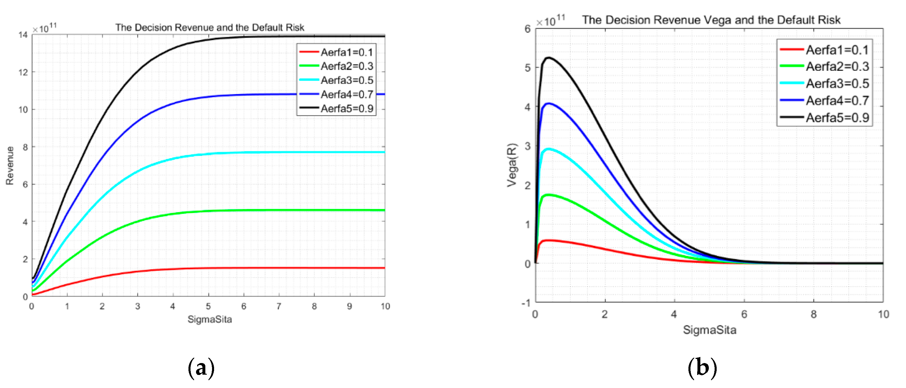
Figure 3a illustrates the decision return value of the bankers with respect to the default risk when the decision structure coefficient varies based on Proposition 1 for Wells Fargo & Co. The image of the inside debt was obtained by fitting the default risk to the corresponding decision return value . Figure 3b illustrates the decision return incentives with respect to the default risk when the decision structure coefficient varies based on Equation (34) of Corollary 1 for the example bank. Similar to Figure 3a, the image of the decision return incentives was obtained by fitting the value to the corresponding value.
As shown in Figure 3a, the volatility of the return on equity has a positive-to-negative influence on the decision return. As a consequence, it has a “risk cap”, where the maximum point in this cap is the optimal risk level to maximize the return of decision-making. Figure 3b shows that the impact of the default risk on the Vega of the decision return becomes stronger and stronger as the decision weight grows.
Figure 4a illustrates the decision return value of the bankers with respect to the decision structure coefficient when the default risk varies based on Proposition 1 for Wells Fargo & Co. The image of the inside debt was obtained by fitting the decision structure coefficient to the corresponding decision return value . Figure 4b illustrates the decision return incentives with respect to the decision structure coefficient when the default risk varies based on Equation (34) of Corollary 1 for the example bank. Similar to Figure 4a, the image of the decision return incentives was obtained by fitting the decision structure coefficient to the corresponding value.
As shown in Figure 4a, the decision weight has a positive influence on the decision return. Furthermore, this effect becomes weaker and weaker as the default risk grows. Figure 4b shows that the decision weight has different directions of influence on the Vega of the decision return as the risk value varies.
Figure 5a illustrates the minimum point and the maximum point of the default risk with respect to the decision structure coefficient based on Equations (35) and (36) of Corollary 1 for Wells Fargo & Co. The image of the minimum point was obtained from Equation (35) (Figure 5a, blue dotted line), and the image of the maximum point was directly drawn by Equation (36) (Figure 5a, orange-red solid line).
Figure 5b illustrates and with respect to the number of periods when based on Equations (51) and (52) of Corollary 3 for the example bank. Similar to Figure 5a, the image of was obtained from Equation (51) (Figure 5b, blue dotted line), and the image of was directly drawn using Equation (52) (Figure 5b, orange-red solid line).
As shown in Figure 5a, the decision weight value yields a negative impact on the optimal risk value . Based on Figure 5b, Equation (57), and Corollary 3, when , the decision weight reaches its optimal value to maximize the decision return value.
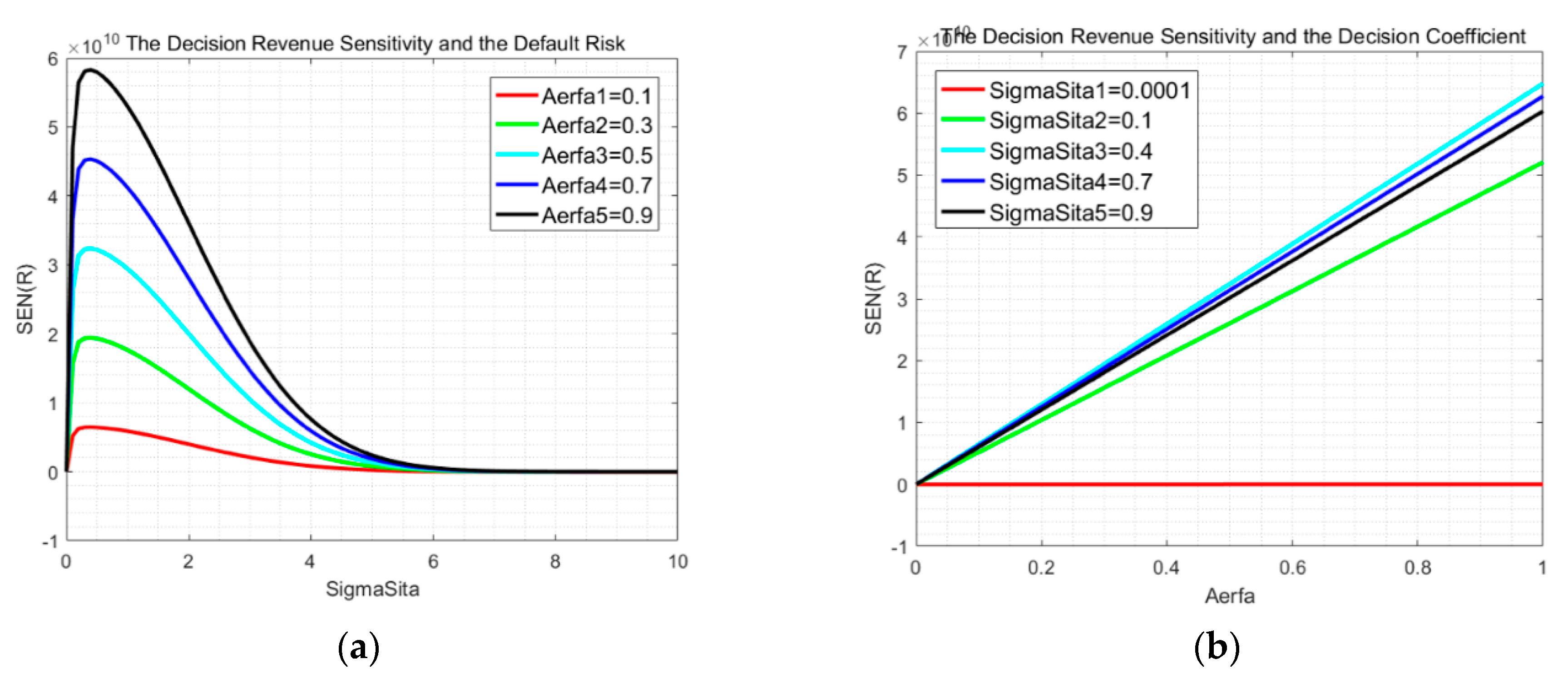
Figure 6a illustrates the sensitivity of the decision revenue of the bankers with respect to the default risk when the decision structure coefficient varies based on Equation (48) and Corollary 2 for Wells Fargo & Co. The image of the sensitivity of the decision revenue was obtained by fitting the default risk to the corresponding value. Figure 6b illustrates the sensitivity of the decision revenue of the bankers with respect to the decision structure coefficient when the default risk varies based on Equation (48) and Corollary 2 for the example bank. Similar to Figure 6a, the image of the sensitivity of the decision revenue was obtained by fitting the decision structure coefficient to the corresponding value.
As shown in Figure 6a, the impact of the default risk on the sensitivity of the decision return becomes stronger and stronger as the decision weight grows. Figure 6b shows that the decision weight has different directions of influence on the sensitivity of the decision return as the risk value varies.
4.3. Robustness
We used the data of Richard M. Adams, Sr. of United Bankshares to perform the robust test. He has been the chairman and CEO of United Bankshares since 1 January 1984. The results showed that our conclusion is robust and effective. The trends and relationships of the decision return, the decision structure, and the default risk are still established. For instance, Equations (63)–(65) are good fits for equations (20)–(22) where United Bankshares is concerned.
5. Conclusions
In this research, we built a multi-stage decision-making model, containing option investment and bond investment, to explore the mechanism of how compensation influencing on risk, based on our previous work (Ma et al., 2020 [22,23]) on a banker’s long-term compensation and the design of pay contracts. As is shown in Table A1 of Appendix A, we illustrated the relationship between the decision return of multi-stages and both the bank’s default risk and decision weight by formulating a particular formula. After setting up the model, we analyzed the function image results using data from Wells Fargo & Co. Firstly, we found an optimal situation regarding the default risk of the bank to maximize the banker’s decision return in multi-stages of option investment and bond investment. Secondly, we were the first to find the presence of a “risk cap”, where the maximum point in this cap is the optimal risk level to maximize the return of decision-making. At the same time, we were the first to determine the optimal decision structure (to invest option or bond more) to maximize the decision return, during which the internal causes and mechanisms of the impact of the banker’s compensation on the bank’s default risk were revealed. Thirdly, this decision-making model sheds light on further theoretical analysis, because it provides a route to bridge the gap of the relationship between the compensation of the banker and the bank’s risk-taking. Fourthly, based on this model, we were able to explain how the banker’s decision influences the decision return and further influences the risk and future compensation, as shown in Figure 1. The limitation of our study is that the banker’s decision of investment contained option investment and bond investment, but did not include other kinds of investment that were difficult to express using the particular formula. We will focus on the particular influence of the decision-making of the banker on the relationship between compensation and the default risk of banks, and we will improve the long-term compensation models by adding an equity incentive.
Author Contributions
Conceptualization, T.M. and M.J.; methodology, T.M.; software, T.M.; validation, T.M., M.J., and X.Y.; formal analysis, T.M.; investigation, T.M.; resources, T.M.; data curation, T.M.; writing—original draft preparation, T.M.; writing—review and editing, T.M., M.J., and X.Y.; visualization, T.M.; supervision, M.J.; project administration, X.Y.; funding acquisition, M.J. All authors have read and agreed to the published version of the manuscript.
Funding
This research was funded by the National Natural Science Foundation of China, grant number 71502044, and the China Postdoctoral Science Foundation, grant number 2015M570300.
Acknowledgments
The authors acknowledge Fu Zhenwu of Harbin Institute of Technology for the given help regarding the MATLAB software.
Conflicts of Interest
The authors declare no conflicts of interest.
Appendix A

Table A1.
Main conclusions of this paper.
| Decision | Definition | Long-Term Model | Relationship with Risk/Decision Structure/Number of Periods | |||
|---|---|---|---|---|---|---|
| From Predecessors or Intuition | From Theoretical Analysis | From Simulation or Empirical Results | Corresponding Figure | |||
| Equation (12): | Proposition 1: | Corollary 1: is increased by in and decreased in and where Equation (44) | Figure 3a and Figure 5a | |||
| Return on decision of option investment | Equation (6): | Equation (30): | Equation (31): | Figure 2b | ||
| Return on decision of bond investment | Equation (9): | Equation (32): | Equation (33): | Figure 2b | ||
| Vega of return on decision | Equation (34): | Corollary 4: | Figure 3b and Figure 5b | |||
| Sensitivity of return on decision | Equation (48): | Corollary 2: | Figure 6a,b | |||
| Decision structure incentives | Equation (50): | Corollary 3: is increased when and decreased when where Equation (57) | Figure 4a,b | |||
Note: stands for a positive relationship between the two variables, stands for a negative one, and stands for an unknown one; is the optimal default risk level to maximize the decision return when is fixed, and is the optimal decision structure level to maximize the decision when is fixed.
References
- Jensen, M.C.; William, H.M. Theory of the firm: Managerial behavior, agency cost, and ownership structure. J. Financ. Econ. 1976, 3, 305–360. [Google Scholar] [CrossRef]
- Wang, T.C.; Lin, Y.L. Using a Multi-Criteria Group Decision Making Approach to Select Merged Strategies for Commercial Banks. Group Decis. Negot. 2009, 18, 519–536. [Google Scholar] [CrossRef]
- Riachi, I.; Schwienbacher, A. Securitization of corporate assets and executive compensation. J. Corp. Financ. 2013, 21, 235–251. [Google Scholar] [CrossRef]
- Li, H.; Henry, D.; Chou, H.I. Stock Market Mispricing, Executive Compensation and Corporate Investment: Evidence from Australia. J. Behav. Financ. 2011, 12, 131–140. [Google Scholar] [CrossRef]
- Latham, S.; Braun, M.R. To IPO or Not To IPO: Risks, Uncertainty and the Decision to Go Public. Brit. J. Manag. 2010, 21, 666–683. [Google Scholar] [CrossRef]
- Kokkinis, A. Exploring the effects of the ‘bonus cap’ rule: The impact of remuneration structure on risk-taking by bank managers. J. Corp. Law Stu. 2019, 19, 167–195. [Google Scholar] [CrossRef]
- Kim, M.S. Study on the Effects of CEO compensation in Investment and earnings management. Manag. Inf. Syst. Rev. 2015, 34, 179–196. [Google Scholar]
- Kang, S.H.; Kumar, P.; Lee, H. Agency and corporate investment: The role of executive compensation and corporate governance. J. Bus. 2006, 79, 1127–1147. [Google Scholar] [CrossRef]
- Huang, H.H.; Huang, H.; Shih, P.T. Real options and earnings-based bonus compensation. J. Bank. Financ. 2012, 36, 2389–2402. [Google Scholar] [CrossRef]
- Ho, P.H.; Huang, C.W.; Lin, C.Y.; Yen, J.F. CEO overconfidence and financial crisis: Evidence from bank lending and leverage. J. Financ. Econ. 2016, 120, 194–209. [Google Scholar] [CrossRef]
- Gulati, A.; Yasin, M.M. DECISION-SUPPORT IN COMMODITIES INVESTMENT - AN EXPERT-SYSTEM APPLICATION. Ind. Manag. Data Syst. 1994, 94, 23–27. [Google Scholar] [CrossRef]
- Grundy, B.D.; Li, H. Investor sentiment, executive compensation, and corporate investment. J. Bank. Financ. 2010, 34, 2439–2449. [Google Scholar] [CrossRef]
- Eisdorfer, A.; Giaccotto, C.; White, R. Capital structure, executive compensation, and investment efficiency. J. Bank. Financ. 2013, 37, 549–562. [Google Scholar] [CrossRef]
- Eastburn, R.W.; Boland, R.J., Jr. Inside banks’ information and control systems: Post-decision surprise and corporate disruption. Inf. Organ. 2015, 25, 160–190. [Google Scholar] [CrossRef]
- Bliss, R.T.; Rosen, R.J. CEO compensation and bank mergers. J. Financ. Econ. 2001, 61, 107–138. [Google Scholar] [CrossRef]
- Belkhir, M.; Boubaker, S. CEO inside debt and hedging decisions: Lessons from the US banking industry. J. Int. Financ. Mark. Inst. Money 2013, 24, 223–246. [Google Scholar] [CrossRef]
- Sheikh, S. CEO inside debt, market competition and corporate risk taking. Int. J. Manag. Financ. 2019, 15, 636–657. [Google Scholar] [CrossRef]
- Li, Z.F.; Lin, S.; Sun, S.; Tucker, A. Risk-adjusted inside debt. Glob. Financ. J. 2018, 35, 12–42. [Google Scholar] [CrossRef] [Green Version]
- Li, Y.; Zhang, X.-Y. Impact of board gender composition on corporate debt maturity structures. Eur. Financ. Manag. 2019, 25, 1286–1320. [Google Scholar] [CrossRef]
- Merton, R.C. On the Pricing of Corporate Debt: The Risk Structure of Interests Rates. J. Financ. 1974, 29, 449–470. [Google Scholar]
- Abad-Segura, E.; Cortés-García, F.J.; Belmonte-Ureña, L.J. The Sustainable Approach to Corporate Social Responsibility: A Global Analysis and Future Trends. Sustainability 2019, 11, 5382. [Google Scholar] [CrossRef] [Green Version]
- Ma, T.; Jiang, M.; Yuan, X. Pay Me Later is Not Always Positively Associated with Bank Risk Reduction—From the Perspective of Long-Term Compensation and Black Box Effect. Sustainability 2020, 12, 35. [Google Scholar] [CrossRef] [Green Version]
- Ma, T.; Jiang, M.; Yuan, X. Cash Salary, Inside Equity or Inside Debt?—The Determinants and Optimal Value of Compensation Structure in a Long-term Incentive Model of Banks. Sustainability 2020, 12, 666. [Google Scholar] [CrossRef] [Green Version]
- Black, F.; Scholes, M. The Pricing of Options and Corporate Liabilities. J. Political Econ. 1973, 81, 637–654. [Google Scholar] [CrossRef] [Green Version]
- Dividend Discount Model. Available online: https://www.investopedia.com/terms/d/ddm.asp (accessed on 10 January 2020).
- Jokivuolle, E.; Keppo, J.; Yuan, X. Bonus Caps, Deferrals and Bankers’ Risk-Taking. Manag. Sci. under review.
- Vuolteenaho, T. What Drives Firm-Level Stock Returns? J. Financ. 2002, 57, 233–264. [Google Scholar] [CrossRef] [Green Version]
- International Monetary Fund. Risk-taking by banks: The role of governance and executive pay. In Global Financial Stability Report: Risk-Taking, Liquidity, and Shadow Banking: Curbing Excess while Promoting Growth; IMF: Washington, DC, USA, 2014. [Google Scholar]
- Gopalan, R.; Milbourn, T.; Song, F.; Thakor, A.V. The Optimal Duration of Executive Compensation: Theory and Evidence. AFA 2012 Chicago Meetings Paper. Available online: http://ssrn.com/abstract=1656603 (accessed on 10 November 2019).
- Sundaram, P.K.; Yermack, D.L. Pay me later: Inside debt and its role in managerial compensation. J. Financ. 2007, 62, 1551–1588. [Google Scholar] [CrossRef] [Green Version]
Figure 1.
Schematic diagram of the effect of the decision-making of bankers on the relationship between compensation and the default risks of banks. (Figure 1 was created by the author of this article according to the framework of the decision-making model presented in this paper).
Figure 1.
Schematic diagram of the effect of the decision-making of bankers on the relationship between compensation and the default risks of banks. (Figure 1 was created by the author of this article according to the framework of the decision-making model presented in this paper).
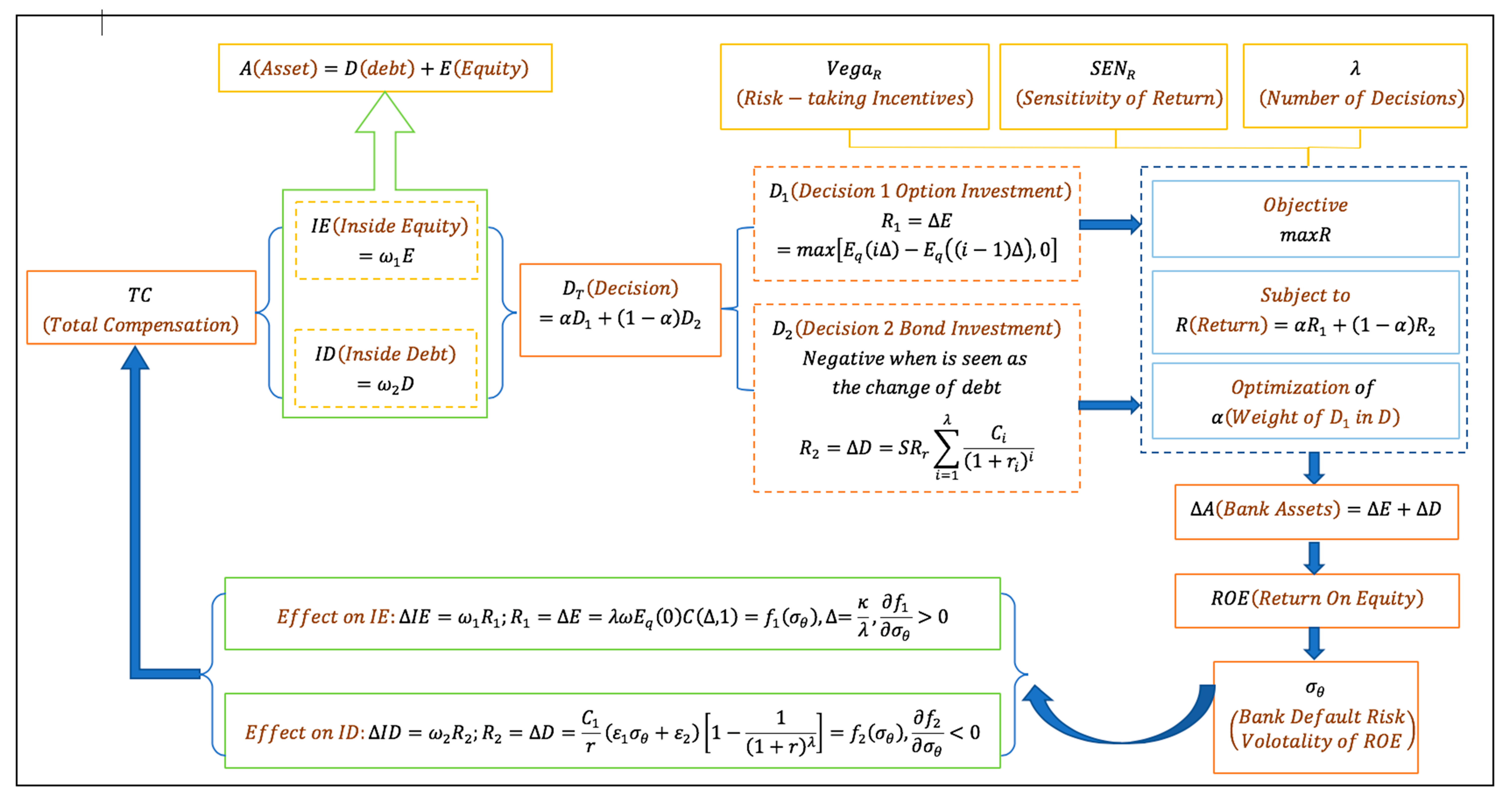
Figure 2.
(a) Function image of the volatility of stock return ratio and the corresponding stock return ratio with respect to the default risk based on Equations (60) and (62) (Note: Parameter values (example bank: Wells Fargo & Co., year: 2015): ); (b) Function image of the decision return of the option investment and the corresponding bond investment with respect to the default risk based on Equations (30) and (32) (Note: Parameter values (example bank: Wells Fargo & Co., year: 2015): . The risk-free rate is the mean of the one-month interest rate of national debt during November 2015 in the U.S.).
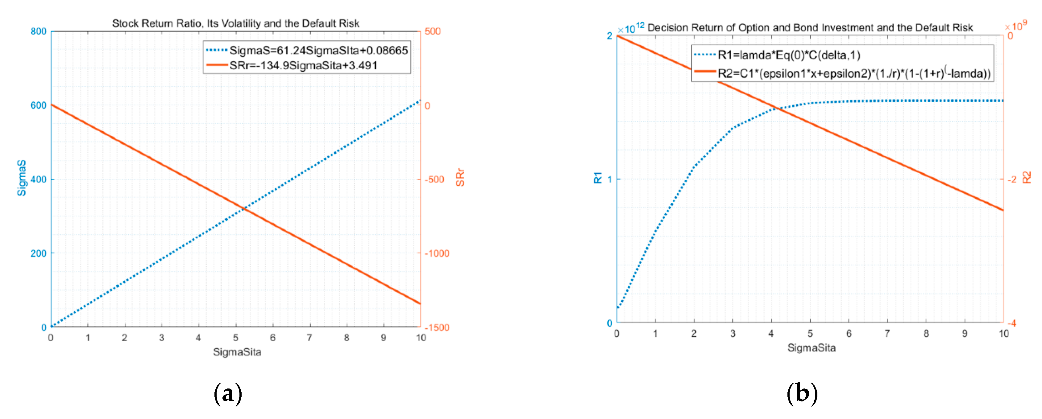
Figure 3.
(a) Function image of the decision return value of the bankers with respect to the default risk when the decision structure coefficient varies based on Proposition 1 (Note: Parameter values (example bank: Wells Fargo & Co., year: 2015): . The risk-free rate is the mean of the one-month interest rate of national debt during November 2015 in the U.S.); (b) Function image of the decision return incentives with respect to the default risk when the decision structure coefficient varies based on Equation (34) of Corollary 1 (Note: Parameter values (example bank: Wells Fargo & Co., year: 2015): . The risk-free rate is the mean of the one-month interest rate of national debt during November 2015 in the U.S.).

Figure 4.
(a) Function image of the decision return value of the bankers with respect to the decision structure coefficient when the default risk varies based on Proposition 1 (Note: Parameter values (example bank: Wells Fargo & Co., year: 2015): . The risk-free rate is the mean of the one-month interest rate of national debt during November 2015 in the U.S.); (b) Function image of the decision return incentives with respect to the decision structure coefficient when the default risk varies based on Equation (34) of Corollary 1 (Note: Parameter values (example bank: Wells Fargo & Co., year: 2015): . The risk-free rate is the mean of the one-month interest rate of national debt during November 2015 in the U.S.).
Figure 5.
(a) Function image of the minimum point and the maximum point of the default risk with respect to the decision structure coefficient based on Equations (35) and (36) of Corollary 1 (Note: Parameter values (example bank: Wells Fargo & Co., year: 2015): . The risk-free rate is the mean of the one-month interest rate of national debt during November 2015 in the U.S.); (b) Function image of and with respect to the number of periods when based on Equations (51) and (52) of Corollary 3 (Note: Parameter values (example bank: Wells Fargo & Co., year: 2015): . The risk-free rate is the mean of the one-month interest rate of national debt during November 2015 in the U.S.).
Figure 6.
(a) Function image of the sensitivity of the decision revenue of the bankers with respect to the default risk when the decision structure coefficient varies based on Equation (48) and Corollary 2 (Note: Parameter values (example bank: Wells Fargo & Co., year: 2015): . The risk-free rate is the mean of the one-month interest rate of national debt during November 2015 in the U.S.); (b) Function image of the sensitivity of the decision revenue of the bankers with respect to the decision structure coefficient when the default risk varies based on Equation (48) and Corollary 2 (Note: Parameter values (example bank: Wells Fargo & Co., year: 2015): . The risk-free rate is the mean of the one-month interest rate of national debt during November 2015 in the U.S.).

Table 1.
Notations and definitions in theoretical analysis.
| Classification | Notations | Definition | Notations | Definition | Notations | Definition | Notations | Definition | Notations | Definition |
|---|---|---|---|---|---|---|---|---|---|---|
| Bank | the bank asset | the bank equity | the bank debt | return on equity | volatility of ROE | |||||
| Compensation | total long-term compensation | inside equity | inside debt | the fraction of equity | the fraction of debt | |||||
| Decision | the banker’s decision-making | option investment | bond investment | the fraction of | return on | |||||
| Option investment | return on | the time interval | the executive’s tenure | the bank equity | number of decision stages | |||||
| Black and Scholes call option price | strike price of the call option | standard cumulative normal distribution | standard normal density | the risk-free rate | ||||||
| Bond investment | return on | cash flow for period | the stock return ratio | slope in Equation (23) | intercept in Equation (23) | |||||
| slope in Equation (21) | intercept in Equation (21) | slope in Equation (22) | intercept in Equation (22) | volatility of stock return ratio | ||||||
| Optimization | Vega of decision return | sensitivity of decision return | decision structure incentives | minimum point of | maximum point of | |||||
| option investment | bond investment | for the monotonicity of | For the monotonicity of | part of expression of | ||||||
| optimal default risk | optimal decision structure | sum of squares due to error | coefficient of determination | root mean square error |
Note: The notation in classification bank and in option investment are both the bank equity; in classification option investment and in optimization are both the decision of option investment; in classification bond investment and in optimization are both the decision of bond investment.
Table 2.
John G. Stumpf’s decision-related variables as CEO of Wells Fargo & Co. ($).
| Year | Age | ||||||
|---|---|---|---|---|---|---|---|
| 2007 | 53 | 99,539.5094 | 2.41 | - | 0.2443 | - | 47,432,000,000 |
| 2008 | 54 | 124,660.0419 | 0.7 | 1.46205 | 0.0324 | 0.022451 | 70,949,000,000 |
| 2009 | 55 | 139,771.0888 | 1.76 | 0.5618 | 0.1574 | 0.007813 | 105,846,000,000 |
| 2010 | 56 | 163,078.1502 | 2.23 | 0.11045 | 0.1486 | 0.0000387 | 119,155,000,000 |
| 2011 | 57 | 145,037.5867 | 2.85 | 0.1922 | 0.167 | 0.000169 | 130,189,000,000 |
| 2012 | 58 | 180,002.6125 | 3.4 | 0.15125 | 0.1792 | 0.0000744 | 145,953,000,000 |
| 2013 | 59 | 238,675.2002 | 3.95 | 0.15125 | 0.1908 | 0.0000673 | 154,646,000,000 |
| 2014 | 60 | 283,438.5322 | 4.17 | 0.0242 | 0.1829 | 0.0000312 | 166,075,000,000 |
| 2015 | 61 | 276,808.1324 | 4.18 | 0.00005 | 0.1735 | 0.0737 | 171,567,000,000 |
| 2016 | 62 | 276,437.767 | 4.03 | 0.01125 | 0.1602 | 0.0000884 | 175,820,000,000 |
Table 3.
The determination of parameters in Equations (20)–(22).
| Curving Fitting | a | b | c | |
|---|---|---|---|---|
| Corresponding Equation | (20) | (21) | (22) | |
| Fit slope | ||||
| Fit intercept | ||||
| Goodness of fit | 0.03544 | 3.188 | 3.953 | |
| 0.9799 | 0.7413 | 0.6791 | ||
| 0.977 | 0.7043 | 0.6333 | ||
| 0.07116 | 0.6748 | 0.7515 | ||
Note: Goodness of fit contains: (a) : the sum of squares due to error; (b) : coefficient of determination; (c) : degree-of-freedom adjusted coefficient of determination; (d) : root mean square error.
© 2020 by the authors. Licensee MDPI, Basel, Switzerland. This article is an open access article distributed under the terms and conditions of the Creative Commons Attribution (CC BY) license (http://creativecommons.org/licenses/by/4.0/).
Share and Cite
MDPI and ACS Style
Ma, T.; Jiang, M.; Yuan, X. Optimize the Banker’s Multi-Stage Decision-Making and the Mechanism of Pay Contract Influencing on Bank Default Risk in the Long-Term Model. Sustainability 2020, 12, 1400. https://doi.org/10.3390/su12041400
AMA Style
Ma T, Jiang M, Yuan X. Optimize the Banker’s Multi-Stage Decision-Making and the Mechanism of Pay Contract Influencing on Bank Default Risk in the Long-Term Model. Sustainability. 2020; 12(4):1400. https://doi.org/10.3390/su12041400
Chicago/Turabian StyleMa, Tianyi, Minghui Jiang, and Xuchuan Yuan. 2020. "Optimize the Banker’s Multi-Stage Decision-Making and the Mechanism of Pay Contract Influencing on Bank Default Risk in the Long-Term Model" Sustainability 12, no. 4: 1400. https://doi.org/10.3390/su12041400
Note that from the first issue of 2016, this journal uses article numbers instead of page numbers. See further details here.