Abstract
This research aims to investigate the extent and nature of productivity growth in manufacturing industries using nonparametric frontier techniques. In order to decompose the total factor productivity (TFP) into technical efficiency change and technological change we use the output-oriented Malmquist productivity index method for 34 Tunisian manufacturing industries over the period 2002–2016. The results indicated that TFP has witnessed an average growth of two percent over the period 2002–2016. The productivity growth identified was attributed to the improvements in the technology (or frontier-shift) rather than improvements or changes in the efficiency.
Keywords:
data envelopment analysis method; productivity index of Malmquist; Tunisia; manufacturing industry JEL Classification:
C14; C61; D24; O14; O47
1. Introduction
Since Solow’s pioneering work, many theoretical and empirical studies have tried to analyze the factors explaining economic growth. Most of these studies concluded that productivity growth is the key to sustained economic growth. (See, among others, [1,2,3,4].)
There are two basic approaches used for the measurement of productivity change: The econometric techniques based on the estimation of a production, cost, or some other functions, and the construction of index numbers using non-parametric methods. The initial technique is an explicit function assigned to the production possibility curve which carries out predictions of its parameters using econometrics which utilize empirical inputs and outputs. The technical efficiency outcome is dependent on the functional form which is taken, which if misstated may lead to outcome bias.
The other technique brings out the proposition that aims at finding out the over-all dynamic productivity transformation indices, which uses the data envelopment analysis (DEA)-based productivity index of Malmquist technique. Most methods advocate for a breakdown into two items; one to find out how efficiency has changed—this is indicated by any motion towards the production possibility curve. The other one indicates a change in the technology of the possibility frontier curve.
The aim of this paper is to develop an output based non-parametric methodology using the Malmquist productivity index methods for calculating productivity growth and to apply it to a sample of Tunisian manufacturing industries. The methodology adopted in this study includes the ideas from measurement of efficiency by [5,6].
Farrell [7] came up with an idea that efficiency can be split into two components, namely the ability and competence of allocation, thus showing the ability of an industry to utilize inputs in the most optimal proportions, taking into consideration their cost price and how technically efficient they are, which shows the capability of an industry to generate maximum output with a given input level [8,9,10]. This way of defining technical efficiency has greatly contributed to the emergence of a variety of techniques that can be used to predict practical productivity. Techniques such as data envelopment analysis (DEA) were brought up by scholars such as Charles, Cooper, and Rhodes. The technique utilizes information from quantities of inputs and outputs. In the process, the technique involves measures of the level of productivity that are both input and output oriented Coelli [11,12,13,14]. According to the study in the DEA technique, there is an attempt to define the frontier by looking at the highest increase in the production level. In regard to the output-oriented case of the technique, the strategy seeks to find out the highest possible proportionate reduction in the use of inputs while the level of output remains constant. The discussion has also relied on Malmquist productivity index (MPI) in the examination of changes in productivity level in regard to manufacturing firms in Tunisia. The technique was brought up by personalities such as Caves, Christensen, and Diewert [15,16].
In the output-orientated case, which is used in this study, the DEA method defines frontier by seeking the maximum proportional increase in output production, with input levels held fixed. While, in the input-orientated case, the DEA method seeks the maximum possible proportional reduction in input usage, with output levels held constant. This study uses the Malmquist productivity index (MPI) to examine productivity change in the Tunisian manufacturing industry. The MPI was introduced by [15,16].
Tunisia is one of the developing countries with a vast industrial base. Indeed, during 1980s, Tunisia adopted the industrial policy (IP), aimed initially to put the national economy on a path of high and sustained growth. This policy contributed to a balanced distribution of industrial activities at a regional level and to support the emergence of a structured manufacturing industry. In order to achieve sustained growth, the Tunisian government implemented accompanying policies, mainly the structural adjustment program (PAS) in the mid-1980s and the industrial modernization program (PMI) in 1996. Moreover, the government ensured the openness and trade liberalization by signing the free trade agreement (FTA) with the European Union (EU) in 1995. The major target of the FTA is to improve the productivity of the manufacturing sector and to increase the export share of manufacturing products. In 2017, the Tunisian industrial sector accounted for 30.4% of the GDP. Approximately 5426 manufacturing companies have already set up in the country and are either totally or partially producing for the European, American, and African markets, among others. Forty-seven percent of these companies are joint ventures or foreign-owned. However, productivity growth in the industrial sector has been the subject matter for intense research over the last two decades due to increasing competition and changing economic situations at the global level. The majority of these studies used a panel of six manufacturing industries or a panel of firms in the Tunisian manufacturing sector, which reflected the analysis to a small extent of the industry. To address such issues and to contribute to the research, this study analyzed data collected from 34 major aggregated manufacturing sub-sectors in Tunisia for identifying the productivity change [17,18,19,20].
2. Background Study
Productivity is one of the important factors of growth and measuring productivity is one of the important approaches for determining and evaluating growth and development. According to the Organization of Economic Cooperation and Development (OECD) definition, productivity is the ratio of volume measure of output to a volume measure of input use (OECD, 2001; Schreyer [21]). The purpose of measuring productivity can be attributed to various reasons which include the following.
- ➢
- Technology: Defined as a technique that can be used to translate inputs into outputs that are required for use in different economies. Technology simplifies work and seeks to make products more useful than they were. For instance, extraction manufacturing of raw materials (Griliches, [22]).
- ➢
- Efficiency: Defined as a production process that makes use of maximum output while utilizing the currently available technology with a given level of inputs that happen to be constant. A production process can be defined to be efficient if it covers the above definition. It can thus be said that technical efficiency is meant to reduce the inefficiencies that might occur in a production process [23].
- ➢
- Real cost savings: It is a very efficient way of defining the level of productivity change (Harberger [24]).
- ➢
- Benchmarking processes of production: In this highly competitive world, it is essential to adopt this practice to identify inefficiencies and compare productivity measures with others in order to identify the competitive position and the measures needed for improving productivity (OECD, 2001).
- ➢
- Living standards: Measuring productivity is among the key elements that can be used to measure and assess the levels of living standards.
There are a number of techniques that can be used to measure the level of productivity change. Productivity measures can be classified into single factor productivity measures (measure of output to a single measure of input); and multifactor productivity measure (measure of output to multiple measures of input) [25]. Single factor productivity measures usually include labor or capital; and multifactor productivity measures include capital and labor, or capital, labor, and intermediate inputs like services, energy, materials, etc. [26]).
The Malmquist index (MI) has gained popularity for measuring productivity change in recent years. A number of studies have shown the effectiveness of the technique in measuring productivity change (Grifell-Tatjé and Lovell [27]). It has also been identified that in the presence of non-constant returns to scale, the Malmquist productivity index does not accurately measure productivity change.
Accordingly, addressing various issues associated with MI, [28] proposed a new way for constructing MI in a global framework which makes use of the lowest level of extrapolation principle on the aggregation of the experienced contemporaneous technologies. It was also found by Pastor and Lovell [29] that the mean MI is not circular and adjacent period components have different measures in productivity change. The authors proposed that a global MI index happens to be circular and gives a single measure of productivity change. A number of studies have been done to implement MI in various international companies.
Other researchers [30] used MI approach for evaluating total factor productivity change across microfinance institutions in the Middle East and North America by investigating 33 institutions and found that overall productivity change was in regress and identified a decline in technological change. Coelli and Rao [14] utilized the DEA approach to find out the MI for evaluating the total factor productivity growth in agriculture across over 93 countries from 1980 to 2000. The shadow prices and value shares that are implicit in the DEA-based Malmquist productivity indices were also derived in the study. Ray and Desli [31] considered various aspects including productivity growth, technical progress, and efficiency change in industrialized countries using MI measures. Similarly, [32] considered a single context of the textile industry on an international scale for measuring the productivity changes using MI from 1995 to 2004 and found only a slight increase in productivity. These studies used MI on a wide scale at an international level or a group of countries, while also limiting to a specific industry, reflecting the wide-scale applicability of MI for measuring productivity, technology, and efficiency change.
Similarly, MI is also used in studies focusing on a particular sector specific to a region or a country which reflected the significant findings. Pharmaceutical and hospital industries in Sweden [33] are used for evaluating productivity developments in recent years. Similarly, they investigated the growth of Norwegian banks’ productivity within the years 1980–1989, reflecting the applicability of MI for measuring productivity during environmental (economic/social/political) changes. Similarly, Price and Weyman-Jones [34] identified a significant increase in the productivity growth of the UK gas industry before and after privatization. Accordingly, MI approach is used for measuring productivity changes/growth across various industries, microfinance institutions in Kenya [35], Malaysian cage fish farming [36] road transport infrastructure in Spain [37], and Nigerian seaports after reform [38], reflecting the applicability of MI approach across various industries.
In the context of Tunisia, there are very few studies found using the concept of MI approach for measuring productivity changes across various sectors. Two studies were identified focusing on the evaluation of productivity changes across the Tunisian schools and educational institutions [39,40,41,42,43]. Zrelli and Belloumi [44] used MI for investigating the impact of environmental strategies on the Tunisian manufacturing industry during 1994–2008 by using data from 26 industries and found an average increase of 1.5% a year. Similarly, technical change and total factor productivity growth in the Tunisian manufacturing industry was evaluated by Kalai and Helali [26] by using data from six industries. They found that the industry achieved poor technological progress rates, and the efficiency gain observed was attributed to improvements in the technology. They observed that the total factor productivity improvement was on an average of 1.93% a year. The research in this area of the Tunisian manufacturing sector is very limited as only two studies were identified in the literature search. Considering these factors and the enhanced applicability of MI approach, this paper investigates productivity change in the Tunisian manufacturing industry.
3. Methodology
This study applies the DEA method and computes the Malmquist index to measure Tunisian’s manufacturing productivity. However, the Malmquist index is demarcated using functions of distance that can be both input and output distance functions. An input distance function depicts the production technology by observing the comparative reduction of the input vector, given an output vector (Coelliet al., 2003). The function of output distance which reflects a maximum proportional expansion of the output vector, given an input vector is an issue that was recognized in this study. To describe the output distance function, a sample of K industry by inputs in the production of outputs in time dated t = 1, …, T is well-thought-out. Multiple inputs and outputs production technology may be defined using the output possibility set, P, which denotes the set of all outputs vectors,, which can be formed using the input vector, through period t = 1, …, T. That is:
Output oriented distance which is also referred to as distance function (Shephard (1970)) is described as follows:
The distance function is equivalent or less than 1 (i.e., D (x, y) ≤ 1), if and only if output y belongs to the production possibility set of x (i.e., y ∈ P (x)). Note that distance function is equivalent to the unit (for instance, D (x, y) = 1) if y belongs to the frontier of the production possibility set. An industry is considered technically effective if the interval function is correspondent to 1.
Now for any given industry in period t, an output-based measure of efficiency can be presumed by the vertical distance ratio ob/oa. The outputs can be increased to make production technically efficient in time t (i.e., movement against the efficient boundary) as shown in Figure 1. By comparison, in vertical distance ratio oe/od in order to realize similar technical efficiency to that originates in time t. Since the frontier has shifted, od/oe exceeds unity, even though it is technically inefficient when compared to the period t + 1 frontier. The MPI measures the total factor productivity (TFP) change between two periods. MPI may be described using an output-oriented method or the input-oriented method. In this study we use the output oriented MPI. Output-orientation refers to the emphasis on the maximum level of outputs that could be produced using a given input vector and a given production technology relative to the observed level outputs. Following Färe and al. (1994), the output oriented MPI between period t (the reference period) and period t + 1 is given by:
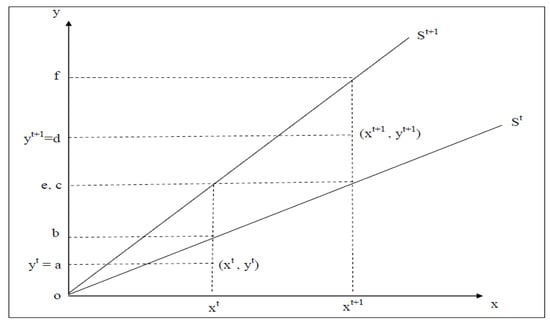
Figure 1.
The Malmquist output-based index and efficiency.
Subscript 0 shows an output-orientation. The notation
represents the distance function from the period t + 1 observation to the period t technology.
MPI is a value in Equation (3). The first ratio signifies the time t Malmquist index and evaluates productivity change from period t to period t + 1 using period t technology as reference. The second ratio represents the period 1 + t Malmquist index and measures productivity change from period t to time t+1 using time t + 1 technology as a reference. Notice that Equation (3) is the geometric mean of first and second ratios. Value of the greater than unity will show positive TFP growth between two periods, whereas a value less than 1 specifies TFP deterioration. According to Färe and al. (1993), the MPI may be decomposed into two components that is an equivalent way of writing this productivity index (Equation(3)) as:
In this equation the fraction outside the bracket calculates the shift in the output-oriented of Farrell technical efficiency over the two periods.
The ratio in the square bracket = calculates the change in technology over the two periods. It is the geometric mean of the change in technology measured at time periods t and t + 1, assessed at xt and also xt+1. Bigger than unity values for the ratios recommend improvement or values less than 1 recommend the contrary. Efficiency change ratio here denotes the enhanced capability of an industry to implement the global technology offered at different time points whereas technical change calculates the consequence of shift in the production frontier resulting from technological advances on industrial output.
MPI in the mathematical Equation (4) comprises four different distance functions ; ; and . Following Färe et al. (1994), and granted that suitable panel data are available, we can calculate these four functions by using DEA linear programs. For each industry, we calculate four distance functions to calculate TFP change between two periods t and t + 1. This requires the solving of four linear programming (LP) problems. Assuming constant returns-to-scale, to begin with, the following output-oriented linear programs are:
where:
and are vectors of output quantities for the i-th industry in period and in period , respectively;
and are vectors of input quantities for the i-th industry in period and in period , respectively;
and are matrixes of output quantities for all N industries in period and in period , respectively;
and are matrixes of input quantities for all N industries in period and in period , respectively;
⅄ is a vector of weights; and is a scalar indicating the technical efficiency score.
It’s good to note that the first two linear programs five and six (LP (5) and (6)) are where the technology and the observation to be evaluated from the same period, and the solution value is less than or equal to 1. The linear programs seven and eight (LP (7) and (8)) occur where reference technology is developed in a one period from the data, whereas the observation to be evaluated is from another period. The parameter should not be greater than or equal to 1, since it should be calculating standard output-oriented technical efficiencies. The data point could lie above the production frontier. Statistically it may lie directly above the construction boundary. This can maximum in LP (8) the point of production from time 1 + t is as compared to technology in an advance epoch. However the technical developments have come about, then a value of theta less than 1 is feasible. This could also likely occur in LP (7) if technical regress has happened, however this is less likely.
For this research, we have utilized the DEA methods to estimate the frontier functions and a data envelopment analysis computer program (DEAP) version 2.1 developed by Coelli (1996) for calculation of Malmquist TFP indexes.
4. Results and Discussion
The data used in this study consist of annual observations of 34 Tunisian manufacturing industries (see Table 1 & Appendix A) for which observations are available over the whole period 2002–2016. The industries included in the study are distributed in six sectors as follows:

Table 1.
Distribution of manufacturing industries.
We note that the industries are distributed as follows across sectors: 26% belong to agriculture and food products (IAF), 12% to the construction materials, ceramics, and glass (CMCG), 24% to the mechanical and electrical industries (MEI), 15% to the chemical industry (CI), 12% to the textile, clothing, and leather industry (TCL), and 12% to other manufacturing industries (OMI).
The data contain data on input and output. We specify variable of yield and incoming variables. Our yield is the cost bought with a market price that is constant. Technology of production is defined as presumptuous of the regular scale of returns: Stock capital and input due to labor is measured for some permanent employees. Statistically they are assembled using a diversity of sources: The general organization of records as well as the quantitative economic system institution, allowing for the construction of an incorporated database. It is worth noting that even though the exertions market became more flexible over the complete duration, the public law for hours worked did now not trade. We expect that the level and the evolution of productivity have been now not raised by using these missing information Pham, T.T et al. (2019), Micieta, et al. (2019), Mark et al. (2019).
The capital stock has been calculated, at constant prices, using the perpetual inventory method for annual investment flows. This method defines the evolution of the capital stock at constant prices as follows:
Where Kt is the capital inventory at the instant t; K (t − 1) is the capital inventory on the spot t −1; It is the funding on the instantaneous t; standard deviation which is a capital depreciation rate.
We have taken into consideration a mean 10% depreciation per year. Our foremost explanation for depreciating prices and productiveness fluctuations never proved to be weighty depreciation charges, as well as the concerned fact absence of the components.
Table 2 shows descriptive statistics of input variable (L). The number of permanent employees increased by 52.5% on average between 2002 and 2016. However, on a year to year base, we observed small changes in the average number of permanent employees.
Table 2.
Descriptive statistics of input variable L (number of permanent employees).
On average, our statistics show an increase in the capital stock during the observed time period by 7.75% (see Table 3). The reason for the increase in capital stock is that some industries have changed from old to new equipment during the period 2002 and 2016.
Table 3.
Descriptive statistics of input variable K (capital stock at a constant price).
Our estimation of value added at constant market prices shows an increase by 83.27% between 2002 and 2016. However, we observe a remarkable increase of 14% between 2007 and 2008 (see Table 4).
Table 4.
Descriptive statistics of output variable VA (value added at constant market prices).
Given that we have 15 annual observations on 34 manufacturing industries, we have a lot of computer output to describe. Our calculations involved the solving of 34 × (15 × 3 − 2) = 1.462 LP problems (Coelli (1996)). We have thousands of pieces of information on the efficiency scores and peers of each industry in each year. We also have measures of technical efficiency change, technical change and TFP change for each industry in each pair of adjacent years. Table 5, Table 6 and Table 7 display the results.
Table 5.
(a) Change (a) in manufacturing industries relative efficiency between time period t and t + 1 (2002 to 2016). Thirty-four Tunisian manufacturing industries; (b) A complement. Change (a) in manufacturing industries relative efficiency between time period t and t + 1(1994 to 2008). Thirty-four Tunisian manufacturing industries.
Table 6.
Shifts (c) in manufacturing industries frontier technology. Averaged geometrically between time period t and t + 1 (2002 to 2016). Thirty-four Tunisian manufacturing industries.
Table 7.
(a) Productivity change (e) in manufacturing industries (annual change between time period t and t + 1 (2002 to 2016). Thirty-four Tunisian manufacturing industries. (b) The complement to Table 7. Productivity change (e) in manufacturing industries (yearly variation amid time phase t and t + 1 (2002 to 2016). Thirty-four Tunisian manufacturing industries.
Table 5 suggests calculated modifications in relative output performance for every individual enterprise and the overall average for all industries. In an output-based model of productiveness exchange quite a value, more than regress value. But, in Table 5, Table 6 and Table 7, we think that improvement in productiveness, as well as improvement in efficiency and time, is indicated by using values greater than 1, while costs less than 1 indicate regress. We are also aware that the mode of LP (l) turned into selected output industry outcome.
The values in Table 5 constitute the period of time not within the Equation (4)’ brackets, for instance changes in competence. For a company that is competent for time t + 1 and for time t maintains its performance relativity. No industry was green in all periods. For the nine industries four, five, eight, nine, 11, 15, 26, 33, and 34, we discovered intervals with declines in performance in addition to periods with upgrades in performance. We discovered no industry with most effective development or only regress in performance at some point of the period 2002 to 2016. For the industries as an whole, five periods confirmed common development in performance, and in nine intervals there was decline in the mean performance. Within the years 2008 and 2009 the total fall in competence is 4.37%. This was observed through a 1.5%development in performance. We checked for minimal changes during the final periods. The bigger shifts inside the frontier from 2003–2004 and 2013–2014 for some industries (20 and four) can be because of errors in pronounced records.
Table 6 presents calculated technical progress/regress as measured by average shifts in the industry frontier from period t to period t + 1. This corresponds to the term in the bracket in Equation (4). Our results showed on average 12 periods with progress and two periods with regress. Between 2007–2008 and 2014–2015 all industries showed technical progress. Here, we note that on average, value added produced by technical staff increased by 13.98% and 7.57%, which may be one explanation for the calculated positive shift in the frontier. The larger shifts in the frontier between 2008–2009 and 2010–2011 for a few industries (manufacture of electric equipment (N°19) and manufacture of oils and other fatty substances (N°4)) may be due to errors in reported data.
On the other hand, for more than half of the industries our calculation showed technical progress of more than 4% between 2007 and 2008. On average we found progress in five periods for the latter part of our study period.
Table 7 summarizes productivity change results in manufacturing industries, that is the evolution of Malmquist output-based productivity index in Equation (4), which is a combination of the efficiency and technical change components, that are discussed above. According to our results, we have had, on average, productivity gains in 13 periods and productivity losses in one period. Again, only three industries (manufacture of electric equipment (N°19), other basic chemical industries (N°23) and para-chemistry (N°24)) showed progress in all periods. For all industries and all periods, we found productivity gains in 366 cases and productivity losses in 110 cases, i.e., progress in 77% of all cases. For the period 2011–2016 we found progress in 81% of all cases. We note that on average, progress in productivity during the five latter years of our study period is mainly explained by positive shifts of the frontier.
Table 8 shows an annual total factor productivity growth of 2%; with technical change (or frontier-shift) contributing 3.1% per year and decline in efficiency change of 1.2%. We can say that during our study period, the increase of productivity is a result of technological progress.
Table 8.
Annual mean technical efficiency change, technical change, and total factor productivity (TFP) change (2002–2016).
In terms of individual industry performance (see Table 9), the most spectacular performance is posted by manufacture of electric equipment (N°19) with an average annual growth of 5.2% in TFP over the study period. Other industries with strong performance are, among others, pharmaceutical industry (N°25) and manufacture of oils and other fatty substances (N°4).
Table 9.
Mean technical efficiency change, technical change, and TFP change (2002–2016).
Table 9 shows the mean technical efficiency change, technical change and TFP change for the 34 industries over the period 2002 to 2016. In terms of individual industry performance, the most spectacular performance is posted by manufacture of electric equipment (N°19) with an average annual growth of 5.2% in TFP, which is due to 5.2% growth in technical change over the study period. Other industries with strong performance are, among others, pharmaceutical industry (N°25) and manufacture of oils and other fatty substances (N°4). The unweighted average (across all industries) growth in TFP is 2%.
Construction materials, ceramic and glass industries (CMCGI); mechanical and electrical industries (MEI); and chemical industries (CHI) are the major performers with an annual TFP growth of 2.6% (mainly due to technical change growth of 3.2%, 3.9%, and 2.2%) followed by other manufacturing industries (OMI), agri-food industries (AFI), and textile, clothing, and leather industries (TCLI). Textile, clothing, and leather industries seem to be the weakest performer with only 1.3% growth in TFP followed by agri-food industries with 1.8% growth in TFP. A surprising result is that over the period 2002–2016, these results show that technical change is the principal source of TFP growth for all sectors as shown in Table 10.
Table 10.
Weighted means of annual technical efficiency change, technical change, and TFP change for the sectors (2002–2016).
Figure 2 shows cumulative TFP indices from 2002 to 2016 for the different sectors. From the figure it is evident that chemical industries have the highest cumulative growth by 2016, followed by mechanical and electrical industries, other manufacturing industries, and clothing and leather industries. Mechanical and electrical industries have a higher cumulative growth than the global growth in TFP. Construction materials, ceramic, and glass industries, and agri-food industries remain as the bottom groups.
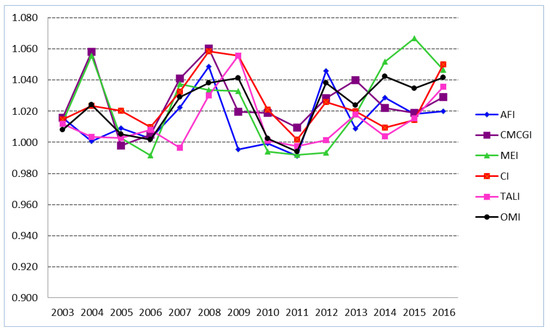
Figure 2.
Cumulative TFP Indices.
For four sectors as shown in Table 11: Other manufacturing industries (OMI); mechanical and electrical industries (MEI); textile, clothing, and leather industries (TCLI); and construction materials, ceramic, and glass industries (CMCGI), the long-run annual average rate of TFP, ranges between 1.306% for textile, clothing, and leather industries and 3.355% for other manufacturing industries over the period 2002–2016. The situation is somewhat different for the two other sectors. In the chemical industries, TFP strongly increases by about 3.470% per year. But, the agri-food industries were characterized by lower rates (0.413%) over the study period.
Table 11.
TFP in six Tunisian manufacturing sectors over the 2002–2016 period.
5. Conclusions
In this paper the productivity growth in 34 Tunisian manufacturing industries over the 2002–2016 period within the framework of the DEA piecewise linear production function and the output-based Malmquist productivity index introduced by Caves, Christensen, and Diewert (1982) is analyzed. This allowed the simultaneous analysis of changes in best-practice due to frontier growth and changes in the relative efficiency of industry to movements towards existing frontiers. The results show that during our study period, the increase of productivity is a result of technological progress. In terms of individual industry performance, the most spectacular performance is posted by manufacture of electric equipment (N°19). Other industries with strong performance are, among others, pharmaceutical industry (N°25) and manufacture of oils and other fatty substances (N°4). Considering the performance of various sectors, construction materials, ceramic, and glass industries (CMCGI); mechanical and electrical industries (MEI); and chemical industries (CHI) are the major performers. Textile, clothing, and leather industries seem to be the weakest performers.
The long run productive performance of Tunisian industries turns to be heterogeneous across sectors and sub-sectors. Some manufacturing activities experience a decline while others strengthen their position and contribute to modify the national production structure. However, these results suffer from a number of limitations. The main limitation is the lack of background or nondiscretionary elements into the study. This oversight is the outcome of insufficient facts and means, and it is difficult to comprehend why the variations in output, competence, and particularly technology, have occurred. Second, the measures of competence and scientific advancement delivered in this reading are best practice, in that the fabrication frontier is a derivative from the illustration itself. There is no information to propose that efficiency modification in manufacturing has not either been commendable nor equivalent to that observed in other manufacturing companies. Lastly, the current reading shares its deterministic appearance in common with other DEA-based methodologies; that is, no opening is made for capacity or condition fault. Nonetheless, the Malmquist index method is exclusively common and can also be instigated in econometric frontiers. This points out a significant space for future research.
Author Contributions
All authors contribute in all works steps and phases equally from beginning to publication. All authors have read and agreed to the published version of the manuscript.
Funding
This research received no external funding.
Acknowledgments
First author would like to thank Deanship of Scientific Research at Majmaah University for supporting this work under the project number No. R-1441-71.
Conflicts of Interest
The authors declare no conflict of interest.
Appendix A
Table A1.
Sample distribution per activities branch.
References
- Afsharian, M.; Ahn, H. The overall Malmquist index: A new approach to measuring productivity changes over time. Ann. Oper. Res. 2014, 226, 1–27. [Google Scholar] [CrossRef]
- Baily, M. Competition, Regulation, and Efficiency in Service Industries. Brook. Pap. Econ. Act. 1993, 1993, 71–159. [Google Scholar] [CrossRef]
- Banker, R.D.; Charnes, A.; Cooper, W.W. Some models for estimating technical and scale inefficiencies in data envelopment analysis. Manag. Sci. 1984, 30, 1078–1092. [Google Scholar] [CrossRef]
- Wolff, E.; Baumol, W.; Blackman, S.A. Productivity and American Leadership: The Long View; MIT Press: Cambridge, MA, USA, 1992. [Google Scholar]
- Yahia, F.B.; Essid, H.; Rebai, S. Do dropout and environmental factors matter? A directional distance function assessment of Tunisian education efficiency. Int. J. Educ. Dev. 2018, 60, 120–127. [Google Scholar] [CrossRef]
- Berg, S.; Førsund, F.; Jansen, E.; Berg, S.; Forsund, F. Malmquist Indices of productivity growth during the Deregulation of Norwegian Banking, 1980–1989. Scand. J. Econ. 1992, 94, S211. [Google Scholar] [CrossRef]
- Farrell, M.J. The measurement of productive efficiency. J. R. Stat. Soc. Ser. A 1957, 120, 253–289. [Google Scholar] [CrossRef]
- Chaffai, M.A.; Plane, P.; Triki, D. Total Factor Productivity in Tunisian Manufacturing Sectors: Convergence or Catch-Up with OECD Members? Working Paper Series N°; The Middle East and North Africa taylor & Francis: Oxford, UK, 2006. [Google Scholar]
- Charnes, A.; Cooper, W.W.; Rhodes, E. Measuring the efficiency of decision-making units. Eur. J. Oper. Res. 1978, 2, 429–444. [Google Scholar] [CrossRef]
- Charnes, A.; Cooper, W.W.; Lewin, A.Y.; Seiford, L.M. Data envelopment analysis theory, methodology and applications. J. Oper. Res. Soc. 1997, 48, 332–333. [Google Scholar] [CrossRef]
- Coelli, T.J.; Rao, D.S. Total Factor Productivity Growth in Agriculture: A Malmquist Index Analysis of 93 Countries 1980–2000; CEPA Working Paper 02/2003; The University of Queensland: Brisbane, Australia, 2003. [Google Scholar]
- Coelli, T.J.; Rao, D.S.P.; O’Donnell, C.J.; Battese, G.E. An Introduction to Efficiency and Productivity; Springer: Berlin, Germany, 1998. [Google Scholar]
- Coelli, T. A Guide to DEAP Version 2.1: A Data Envelopment Analysis (Computer) Program; CEPA Working Paper 96/08; University of New England: Armidale, Australia, 1996. [Google Scholar]
- Coelli, T.; Rao, D. Total factor productivity growth in agriculture: A Malmquist index analysis of 93 countries, 1980–2000. Agric. Econ. 2005, 32, 115–134. [Google Scholar] [CrossRef]
- Caves, D.W.; Christensen, L.R.; Et Diewert, W.E. The economic theory of index numbers and the measurement of input, output, and productivity. Econometrica 1982, 50, 1393–1414. [Google Scholar] [CrossRef]
- Diewert, E.W.; Denis, L. “Measuring New Zealand’sProductivity”, Treasury Working Paper 99/5. 1999. Available online: http://www.treasury.govt.nz/workingpapers/99-5.htm (accessed on 30 May 2018).
- Essid, H.; Ouellette, P.; Vigeant, S. Productivity, efficiency, and technical change of Tunisian schools: A bootstrapped Malmquist approach with quasi-fixed inputs. Omega 2014, 42, 88–97. [Google Scholar] [CrossRef]
- Fare, R.; Grosskopf, S.; Lindgren, B.; Roos, P. Productivity changes in Swedish pharamacies 1980–1989: A non-parametric Malmquist approach. J. Product. Anal. 1992, 3, 85–101. [Google Scholar] [CrossRef]
- Färe, R.; Grosskopf, S.; Lindgren, B.; Roos, P. Productivity Developments in Swedish Hospitals: A Malmquist Output Index Approach. Data Envelopment Analysis: Theory, Methodology, and Applications; Springer: Berlin, Germany, 1994; pp. 253–272. [Google Scholar]
- Färe, R.; Grosskopf, S.; Norris, M.; Zhang, Z. Productivity Growth, Technical Progress, and Efficiency Changes in Industrialized Countries. Am. Econ. Rev. 1994, 84, 66–83. [Google Scholar]
- Schreyer, P. Measuring Productivity. In Proceedings of the OECD Conference on Next Steps for the Japanese SNA Tokyo, Tokyo, Japan, 25 March 2005. [Google Scholar]
- Griliches, Z. Productivity: Measurement Problems. In The New Palgrave: A Dictionary of Economics; Eatwell, J., Milgate, M., Newman, P., Eds.; Palgrave Macmillan: London, UK, 1987. [Google Scholar]
- Nwanosike, F.; Tipi, N.; Warnock-Smith, D. Productivity change in Nigerian seaports after reform: A Malmquist productivity index decomposition approach. Marit. Policy Manag. 2016, 43, 798–811. [Google Scholar] [CrossRef]
- Harberger, A.C. A Vision of the Growth Process. Am. Econ. Rev. 1998, 88, 1–32. [Google Scholar]
- Iliyasu, A.; Mohamed, Z.; Hashim, M. Productivitygrowth, technical change and efficiency change of the Malaysian cage fish farming: An application of Malmquist Productivity Index approach. Aquac. Int. 2014, 23, 1013–1024. [Google Scholar] [CrossRef]
- Kalai, M.; Helali, K. Technical change and total factor productivity growth in the Tunisian manufacturing industry: A Malmquist index approach. Afr. Dev. Rev. 2016, 28, 344–356. [Google Scholar] [CrossRef]
- Grifell-Tatjé, E.; Lovell, C. A note on the Malmquist productivity index. Econ. Lett. 1995, 47, 169–175. [Google Scholar] [CrossRef]
- Kapelko, M.; Lansink, A.O. An international comparison of productivity change in the textile and clothing industry: A bootstrapped Malmquist index approach. Empir. Econ. 2014, 48, 1499–1523. [Google Scholar] [CrossRef]
- Pastor, J.; Lovell, C. A global Malmquist productivity index. Econ. Lett. 2005, 88, 266–271. [Google Scholar] [CrossRef]
- Maroto, A.; Zofío, J. Accessibility gains and road transport infrastructure in Spain: A productivity approach based on the Malmquist index. J. Transp. Geogr. 2016, 52, 143–152. [Google Scholar] [CrossRef]
- Ray, S.C.; Desli, E. Productivity growth, technical progress, and efficiency change in industrialized countries: Comment. Am. Econ. Rev. 1997, 87, 1033–1039. [Google Scholar]
- Morrisson, C.; Talbi, B. La Croissance de L’économie Tunisienne en Longue Période, Etude du Centre de Développement de l’OCDE, Série Croissance; OCDE: Paris, France, 1996. [Google Scholar]
- The Organisation for Economic Co-operation and Development (OECD). Measuring Productivity- OECD Manual- Measurement of Aggregate and Industry-Level Productivity Growth. Available online: https://www.oecd.org/sdd/productivity-stats/2352458.pdf (accessed on 30 May 2018).
- Price, C.; Weyman-Jones, T. Malmquist indices of productivity change in the UK gas industry before and after privatization. Appl. Econ. 1996, 28, 29–39. [Google Scholar] [CrossRef]
- Shephard, R.W. Theory of Cost and Production Functions; Princeton University Press: Princeton, NJ, USA, 1970. [Google Scholar]
- Solow, R.M. Technical Change and the Aggregate Production Function. Rev. Econ. Stat. 1957, 39, 312–320. [Google Scholar] [CrossRef]
- Bassem, B.S. Total factor productivity change of MENA microfinance institutions: A Malmquist productivity index approach. Econ. Model. 2014, 39, 182–189. [Google Scholar] [CrossRef]
- Pham, T.T.; Kuo, T.-C.; Tseng, M.-L.; Tan, R.R.; Tan, K.; Ika, D.S.; Lin, C.J. Industry 4.0 to Accelerate the Circular Economy: A Case Study of Electric Scooter Sharing. Sustainability 2019, 11, 6661. [Google Scholar] [CrossRef]
- Micieta, B.; Binasova, V.; Lieskovsky, R.; Krajcovic, M.; Dulina, L. Product Segmentation and Sustainability in Customized Assembly with Respect to the Basic Elements of Industry 4.0. Sustainability 2019, 11, 6057. [Google Scholar] [CrossRef]
- Mark, B.G.; Hofmayer, S.; Rauch, E.; Matt, D.T. Inclusion of Workers with Disabilities in Production 4.0: Legal Foundations in Europe and Potentials Through Worker Assistance Systems. Sustainability 2019, 11, 5978. [Google Scholar] [CrossRef]
- Wijesiri, M.; Meoli, M. Productivity change of microfinance institutions in Kenya: A bootstrap Malmquist approach. J. Retail. Consum. Serv. 2015, 25, 115–121. [Google Scholar] [CrossRef]
- Zhang, N.; Zhou, P.; Kung, C. Total-factor carbon emission performance of the Chinese transportation industry: A bootstrapped non-radial Malmquist index analysis. Renew. Sustain. Energy Rev. 2015, 41, 584–593. [Google Scholar] [CrossRef]
- Prause, M. Challenges of Industry 4.0 Technology Adoption for SMEs: The Case of Japan. Sustainability 2019, 11, 5807. [Google Scholar] [CrossRef]
- Zrelli, H.; Belloumi, M. Environmental stakeholders, environmental strategies, and productivity of Tunisian manufacturing industries. Middle East Dev. J. 2015, 7, 108–126. [Google Scholar] [CrossRef]


© 2020 by the authors. Licensee MDPI, Basel, Switzerland. This article is an open access article distributed under the terms and conditions of the Creative Commons Attribution (CC BY) license (http://creativecommons.org/licenses/by/4.0/).