Optimal MTS and MTO Hybrid Production System for a Single Product Under the Cap-And-Trade Environment

Abstract

This paper studies the optimal production planning in a hybrid Make-To-Stock (MTS) and Make-To-Order (MTO) production system for a single product under the cap-and-trade environment. The manufacturer aims to minimize the total cost in production, inventory and emissions allowances trading. The decisions include the selection of production mode (pure MTS, pure MTO or hybrid MTS/MTO), the inventory and emissions trading quantity. We derive the optimal solution analytically. We show that the cost of optimal MTO/MTS hybrid production strategy is remarkably less than that of either pure MTO or pure MTS production strategy alone. Compared with the no initial carbon quota and trading environment, there are significant differences in the optimal production decisions under trading environment. When the emissions cost is a source of costs, the manufacturer has to face more costs pressure even if there is no emissions allowance trading. In particular, the results show that the initial emissions allowance determines the optimal production decision and emissions allowance trading decision in cases where the difference between the inventory cost for per unit product and the delayed delivery cost for per unit order is between the minimum and the maximum emissions cost and has no effect on production mode and emissions allowances trading decision in other cases. These conclusions will provide optimal production decision and carbon trading decision for the manufacture under a cap-and-trade environment.

1. Introduction

Since the 1960s, many scholars have paid close attention to two typical modes of production, i.e., Made-To-Stock (MTS) and Made-To-Order (MTO). If a finished goods inventory is held for a product, we say that the product is produced in an MTS mode. Otherwise, we say that the product is produced in an MTO mode ([1]). As [2] indicate, most research in this field has mainly assumed one of the two strategies. For MTS, it is generally believed that this mode can keep inventory levels to avoid stockout, maintain a higher level of service, and reduce the delivery lead time, but incurs a certain amount of inventory cost (see, e.g., [3,4,5]). It is suitable for low value, high stability demands and standardized products. On the other hand, the MTO mode initiates production only after receiving the order and there is no inventory cost (see, e.g., [6,7]), but a longer delivery lead period is expected. The MTO strategy is suitable for products of low service level requirement, high value, and high demand variability (see, e.g., [8,9,10,11], etc.). Considering the significant differences for MTS and MTO production in planning and control decisions, references [10,12] indicate that planning of a hybrid production system is not straightforward.

However, in practice, quite a number of manufacturers use hybrid MTS/MTO mode in production. As [13] emphasized, a proper combination of MTO and MTS can exploit the advantages of both lower inventory and short delivery time. In particular, when the manufacturer faces the standardization requirement and customized lead time requirement simultaneously, mixed production mode becomes more attractive ([4]). For a hybrid MTS/MTO production system, one research directions focus on multi-product systems. In these hybrid MTS/MTO production systems, it is assumed that each product is either pure MTS or pure MTO. For example, [10,14,15] use Markov Decision Processes (MDP) to decide whether MTO or MTS should be chosen. [16,17] develops a nonlinear integer programming for this problem. [18] propose scheduling methods for hybrid MTS/MTO semiconductor fabrication. The other focus on the position of the decoupling point (DP) for MTO and MTS production modes for a single product. [8] adopts the DP concept to the specific characteristics of the food processing industry and develops a frame for a decision which products have to be made to stock and which products have to be made to order. [19] pointed out that market, product and production are the factors that affect the DP positioning and the shifting of the DP upstream or downstream in the manufacturing value chain. [20] extends previous research into a supply network and answers how to position the multiple DPs in a supply network quantitatively. In this paper, we consider a hybrid MTS/MTO production mode for a single product (i.e., some seasonal products, etc.). The same as [1], we assume that the product is not customized. In other words, the product keeps the same in any production mode. In this production system, the manufacturer has to balance the holding cost and service level.

The current globalization is faced by the challenge to meet the continuously growing worldwide demand for capital and consumer goods by simultaneously ensuring a sustainable evolvement of human existence in its social, environmental and economic dimensions ([21]). In the last decade, because the emphasis on adopting eco-friendly practices, implementing sustainability measures, and protecting the environment has continued to grow, many SMEs are now adopting sustainable manufacturing practices ([22]). In the existing studies, scholars often make MTS, MTO or hybrid MTO/MTS production decisions based on production cost, inventory cost, and shortage cost in order to minimize total cost or maximize total profit (see, e.g., [16,23,24]). However, they do not take the effects of emissions allowances trading into consideration. In fact, production activities of manufacturers is one of the main sources of emissions and it is very important to guarantee a balance between socio-economic development and environmental conservation ([25]). How to reduce emissions become a primary target of manufacturers as the emphasis on environment increases. For instance, in order to achieve the goal to reduce emissions per GDP Unit by 40–45% in 2020 compared to 2005, Chinese government has established more stringent regulations for manufacturers to reduce emissions. It has successfully cut down the Energy Intensity per GDP Unit by 16%, and reduced the Carbon Intensity (Carbon Dioxide Emissions per GDP Unit) by 17% in 2011–2015. Researches show that the cap-and-trade is considered to be one of the most effective market-based carbon emission reduction mechanisms ([26]), which has been widely adopted by the United Nations and the European Union. On 19 December 2017, China fully launched the national carbon emission trading market, making it the world’s largest carbon trading market with an initial coverage of over 1700 enterprises and 3 billion tons of carbon emissions. Under the emissions trading mechanism, emissions trading has become a potential profit source to enterprises. Clearly, it will change the cost structure and profit model, and ultimately affect the manufacturers’ production behaviors. Therefore, it is worth discussing the influence of emissions trading mechanism upon the production strategy.

In studies on emissions, the emissions trading price is introduced into the objective function. Some scholars assume that the emissions trading price is exogenous and definite, and the prices of buying and selling are the same (e.g., [27,28]). Some scholars take into account bid-ask price spreads for emissions trading, i.e., different buying and selling prices, and study the impact of emissions reduction mechanism in production. For example, [29] model different selling and buying prices of the allowances and introduce emissions cost as an additional cost of green technology, and set up a multi-period dynamic production planning model under stochastic demands and allowance prices. They determine the optimal production quantity and technical selection scheme based on the impact of emissions trading mechanism on the technology selection and production planning of the manufacturer. On the basis of the studies of [29,30] study the enterprises’ optimal production lot size and optimal emissions under the two mechanisms of emissions trading and emissions tax on EOQ model. They discover that the optimal emissions quantity and emissions trading decisions depend on distinguish price of emissions trading under the emissions trading and allowances system. We adopt emissions trading allowances as a decision variable in the hybrid MTO/MTS production mode of single product on the condition that the initial emissions allowances which price of buying and selling through external market are different.

For single product, it is significant to study the optimal hybrid MTO/MTS production decisions with emissions allowances trading. On the one hand, the hybrid MTO/MTS production decisions for single product can effectively improve the utilization rate of the machine and the level of service. On the other hand, what kind of production mode is adopted to achieve the double goals of economic and environment? The main question is must be answered what is the effects of emissions allowances trading for production decisions because different production mode may deduces different emissions. In order to solve the above problems effectively, we study a hybrid MTS-MTO production for single item under the emissions trading environment in this paper. While most recent researches on hybrid MTS/MTO production use stochastic models, assuming demand (see, [31], etc.), or production times (see, [32], etc.), or lead time (see, [33], etc.) are stochastic, we use a deterministic setting which is similar to the earlier papers on inventory optimization (see, [34], etc.) because it is difficult to get the boundary conditions for optimal production and carbon trading decisions in a random situation. Importantly, deterministic assumption allows us to find the analytical optimal solution. These analytical solutions can help further research on stochastic factors. The results show that the optimal production decisions are different between emissions allowances trading and no emissions allowances trading, and the initial emissions allowances have remarkable influences on the decisions of production mode. In the emissions allowances trading case, the cost of hybrid MTO/MTS optimal production strategy mode is no greater than pure MTO mode and pure MTS mode. We also get the thresholds of optimal production mode and emissions trading quantity which would give an accurate guidance for the manufacturer.

In the following, the paper will be organized as follows. In Section 2, we introduce the mathematical formulation. In Section 3, we derive the optimal production and emissions trading policies analytically. In Section 4, we compare the differences of optimal production decisions with and without emissions allowances. A numerical study is conducted in Section 5 to demonstrate the analytical results and investigate the impacts of parameters, such as demand, production capacity, inventory capacity, and delivery lead time length. We also compare the hybrid MTO/MTS production mode, the MTO production mode, and the MTS production mode. Finally, we conclude the paper in Section 6.

2. Model

2.1. Model Description

At the beginning of the production planning period, the manufacturer obtains $z_0$ units emissions allowances and makes the hybrid production decision and emissions trading decision. We assume that, regardless of the MTO or MTS mode of production, $\alpha$ units emissions are generated when we produce one unit product. Meanwhile, if the MTS mode of production is adopted, the inventory holding cost is $h^{\prime }$ and inventory emissions is ${\beta }^{\prime }$ for per unit product. During the production planning stage, the manufacturer accepts the orders and pays the delayed delivery cost b for each unit if the manufacturer does not complete the orders within delivery lead times. Considering the reality, we assume that customers allow to pick up the goods several times. After the planning stage, the manufacturer needs to keep a nonnegative balance in its allowances account or otherwise pay a penalty $\pi$ for each unit.

In Figure 1, we illustrate the hybrid MTO/MTS production process. At the moment of $t_0$, the manufacturer makes a production decision and an emissions trading decisions for the entire planning period. We assume that the product stock is 0 at the moment of $t_0$ and $t_1$ is the moment that the manufacturer receives orders of D units. In the period of $[t_0,t_1]$, the manufacturer uses the MTS mode to produce y units products and the product stock changes from 0 to y. In the period of $[t_1,t_2]$, the manufacturer adopts MTO mode to produce ${[D-y]}^{+}$ units products.

2.2. Model Formulation

2.2.1. Emissions Trading Cost

Throughout the planning period, if the decision is to purchase emissions allowances, i.e., $z>z_0$, then the cost is $\mu (z-z_0)$. If the decision is to sell emissions allowances, i.e., $z<z_0$, then the profit is $\nu (z_0-z)$. Thus the emissions transaction cost is $\mu {(z-z_0)}^{+}-\nu {[-(z-z_0)]}^{+}$, where ${\left(X\right)}^{+}=max\{X,0\}$, see [29], etc.

2.2.2. Production Cost

The manufacturer produces y units by the MTS mode and ${(D-y)}^{+}$ units by the MTO mode. In this model, MTO production has the same scale effect as MTS production, so we assume that the production cost of the two production methods are the same. The total production cost consists of $cy$ by the MTS mode and $c{[D-y]}^{+}$ by the MTS mode, i.e., $cy+c{[D-y]}^{+}$, see, [20], etc.

2.2.3. Inventory Cost

Throughout the planning period, the inventory cost for the MTO production is negligible, since the finished product by MTO will temporarily stored and do not enter the storage center and fulfill the orders immediately. The same as [20], the inventory holding cost is defined by monetary value per unit and let $h^{\prime }$ is the holding cost per unit. The amount produced by the MTS mode is y and the average inventory level is $\frac{y}{2}$ in $[t_0,t_1]$. Therefore, the inventory cost is $hy$ where $h=\frac{h^{\prime }}{2}$.

2.2.4. Penalty Cost for the Excess Emissions

At the time of $t_0$, the amount of emissions allowances changes to z after the manufacturer makes the trading decision of emissions allowances. Throughout the planning period, the amount of emissions allowances consumed in the MTS production is $\alpha y$, the amount of emissions allowances consumed by stock is $\beta y$ where $\beta =\frac{{\beta }^{\prime }}{2}$, the amount of emissions allowances consumed in the MTO production is $\alpha {(D-y)}^{+}$, so the total emissions allowances consumed in the planning period is $\alpha y+\alpha {(D-y)}^{+}+\beta y$, and the penalty cost for the excess emissions is $\pi {[\alpha y+\alpha {(D-y)}^{+}+\beta y-z]}^{+}$, see [29], etc.

2.2.5. Penalty Cost for Delayed Delivery

At time $t_1$, the manufacturer receives demand D and order delivery lead time l. For a given production capacity M, the maximum amount of products that could be produced within the lead time l is $Ml$, so the unsatisfied demand is ${[D-(y+Ml)]}^{+}$ and then the penalty cost for delayed delivery is $b{[D-(y+Ml)]}^{+}$, see, [35], etc.

2.2.6. Summary

The total cost is the sum of the above five case cost. We define V as the total cost, represented as:

$$\begin{array}{c}\hfill \begin{array}{ccc}V\hfill & =\hfill & \mu {(z-z_0)}^{+}-\nu {[-(z-z_0)]}^{+}+cy+c{(D-y)}^{+}+hy+b{[D-(y+Ml)]}^{+}+\hfill \\ & & \pi {[\alpha y+\alpha {(D-y)}^{+}+\beta y-z]}^{+}.\hfill \end{array}\end{array}$$

(1)

The optimization problem is:

$$\begin{array}{ll}min\hfill & V\hfill \\ \mathrm{s}.\mathrm{t}.\hfill & y\in [0,a]\hfill \end{array}$$

(2)

where $\nu <\mu <\pi$,$a=min\{Y,(t_1-t_0)M\}$.

3. Optimal Policies

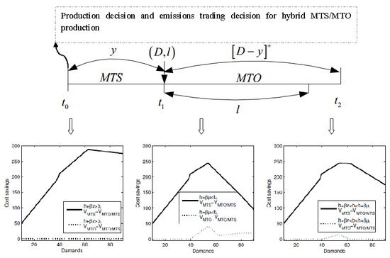
In the manufacturer’s cost function, i.e., Equation (1), we could consider the following situations: 1) Whether the manufacturer decides to buy or sell emissions allowances; 2) whether the products produced in the MTS stage can satisfy the demand for orders; 3) whether the manufacturer exceeds the emissions allowances and pays the penalty of delayed delivery. Based on these situations, we could get the optimal policies analytically:

Theorem 1.

In the planning period, the minimum cost for the manufacturer is:

(i) if $D\le Ml$, then

$$\begin{array}{c}V=\left\{\begin{array}{cc}\mu (\alpha D-z_0)+cD\hfill & 0\le z_0\le \alpha D\hfill \\ \nu (\alpha D-z_0)+cD\hfill & z_0>\alpha D\hfill \end{array}\right.\hfill \end{array}$$

(3)

(ii) if $D>Ml$, then

$$\begin{array}{c}V=\left\{\begin{array}{cc}\mu (\alpha D-z_0)+(D-Ml)b+cD\hfill & 0\le z_0\le \alpha D,h+\beta \mu >b\hfill \\ (\mu \beta +h-b)e+\mu (\alpha D-z_0)+(D-Ml)b+cD\hfill & 0\le z_0\le \alpha D+\beta e,h+\beta \mu <b\hfill \\ \frac{1}{\beta }(h-b)(z_0-\alpha D)+(D-Ml)b+cD\hfill & \alpha D<z_0\le \beta e+\alpha D,\hfill \\ & h+\beta \nu <b<h+\beta \mu \hfill \\ \nu (\alpha D-z_0)+(D-Ml)b+cD\hfill & \alpha D<z_0,h+\beta \nu >b\hfill \\ (\nu \beta +h-b)e+\nu (\alpha D-z_0)+(D-Ml)b+cD\hfill & z_0>\beta e+\alpha D,h+\beta \nu <b\hfill \end{array}\right.\hfill \end{array}$$

(4)

Theorem 1 shows that the minimum cost of a manufacturer can be achieved at various levels of emissions allowances and in different cost boundaries. In the case of lower orders for the product, i.e., $D\le Ml$, the minimum cost of the manufacturer is connected with the initial emissions allowances and emissions from the production of D units. That is, if the initial emissions allowances are less than the emissions for producing D units products, then the minimum cost is $\mu (\alpha D-z_0)+cD$, otherwise, they are $\nu (\alpha D-z_0)+cD$. Moreover, if $D>Ml$, the manufacturer not only needs to consider the level of initial emissions allowances, but also need to make comparison between the delayed delivery cost for unit orders and the sum of the holding cost and the emissions allowances cost for per unit inventory. The minimum cost under different boundary conditions can be shown by Equation (4).

The optimal production decision and emissions trading decision for manufacturer’s minimum cost are as Theorems 2 and 3.

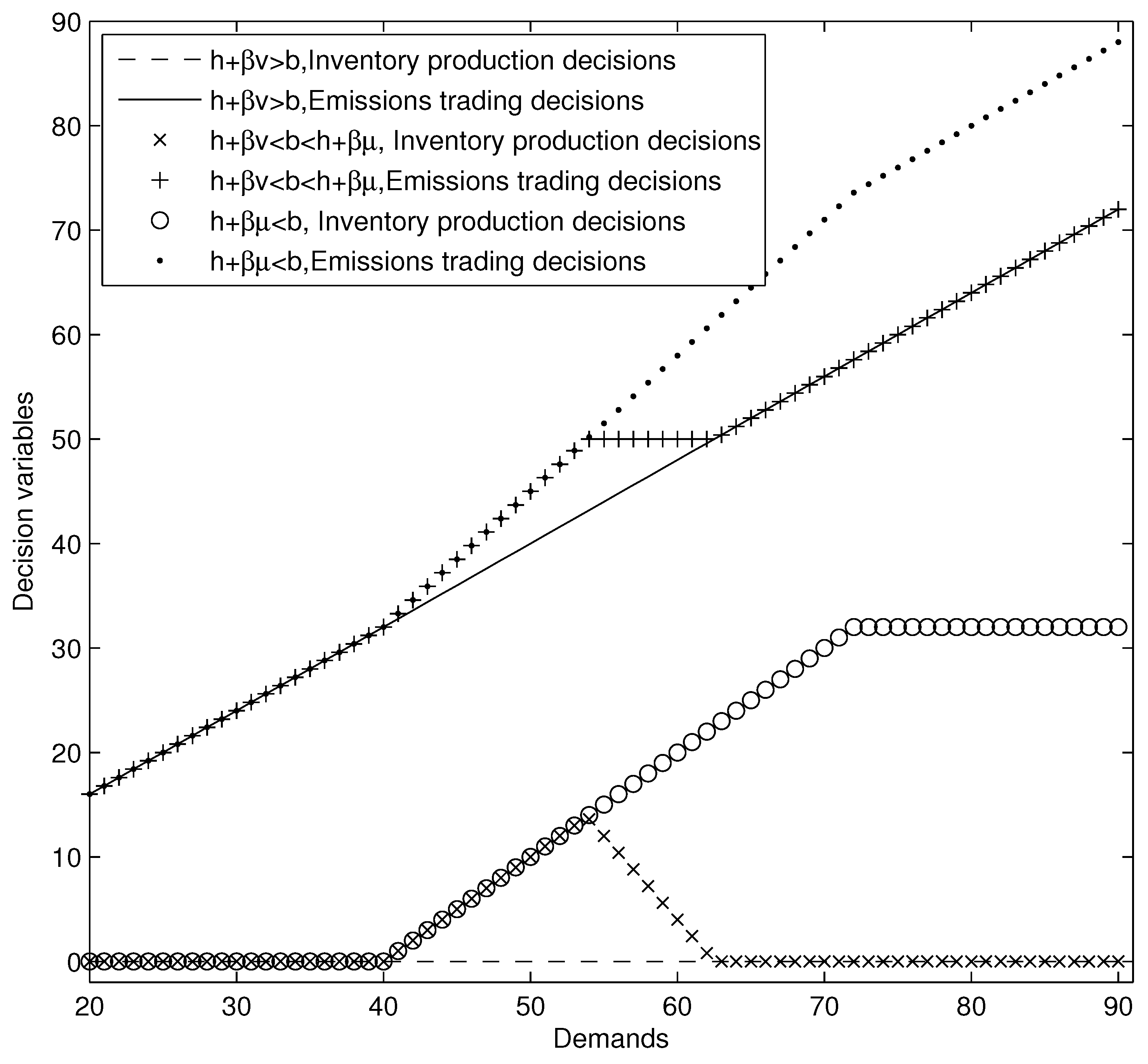
Theorem 2.

In the planning period, manufacturer’s optimal production decisions are as follows:

(i) if $D\le Ml$, then $y=0$;

(ii) if $D>Ml$, then

$$\begin{array}{c}y=\left\{\begin{array}{cc}0\hfill & 0\le z_0\le \alpha D,h+\beta \mu >b,or\alpha D\le z_0,h+\beta \nu >b\hfill \\ e\hfill & 0\le z_0\le \beta e+\alpha D,h+\beta \mu <b,or{z}_0>\beta e+\alpha D,h+\beta \nu <b\hfill \\ \frac{z_0-\alpha D}{\beta }\hfill & \alpha D\le z_0\le \beta e+\alpha D,h+\beta \nu <b<h+\beta \mu \hfill \end{array}\right.\hfill \end{array}$$

(5)

and $e=min(a,D-Ml)$.

According to Theorem 2, when the demand is low, i.e., $D\le Ml$, then the manufacturer’s output meet the orders in the period of lead time, i.e., it chooses not to produce in MTS stage and the production strategy is pure MTO. If $D>Ml$, the manufacturer cannot meet the orders during the period of lead time and need to produce products in MTS stage, then the optimal strategy is a hybrid MTS-MTO production strategy.

If $D>Ml$ and the sum of the MTS holding cost and the maximum emissions cost for per unit inventory are less than the cost of delayed delivery for per unit order, the optimal production decision has nothing to do with the initial emissions allowances, then the optimal hybrid production decision is to produce e units products in the MTS stage. Similarly, if the sum of the MTS holding cost and the minimum emissions cost for per unit inventory are greater than the cost of delayed delivery for per unit order, the optimal production decision has nothing to do with the initial emissions allowances, either. In this case the optimal production decision for MTS stage is produce 0 unit product, and the optimal production strategy becomes the pure MTO strategy. Only when the difference between the inventory cost for per unit product and the delayed delivery cost for per unit order is between the minimum and the maximum emissions cost, the initial emissions allowances affect the production mode and the optimal production decisions. In particular, if the initial emissions allowances are less than the emissions for producing D units products, then the manufacture adopts a pure MTO optimal production strategy; if the initial emissions allowances are greater than the sum of emissions for keeping e units stock and producing D units production, then the manufacture adopts the optimal hybrid MTO/MTS production strategy and produces e units products in MTS stage. Otherwise, it adopts the optimal hybrid MTO/MTS production strategies and products $\frac{z_0-\alpha D}{\beta }$ units products in MTS stage.

Theorem 3.

During the planning period, the optimal emissions allowances trading decisions of the manufacturer are as follows:

(i) if $D\le Ml$, then $z=\alpha D$;

(ii) if $D>Ml$, then

$$\begin{array}{c}z=\left\{\begin{array}{cc}\alpha D\hfill & 0\le z_0\le \alpha D,h+\beta \mu >b,or\alpha D\le z_0,h+\beta \nu >b\hfill \\ \beta e+\alpha D\hfill & 0\le z_0\le \beta e+\alpha D,h+\beta \mu <b,or{z}_0>\beta e+\alpha D,h+\beta \nu <b\hfill \\ z_0\hfill & \alpha D\le z_0\le \beta e+\alpha D,h+\beta \nu <b<h+\beta \mu \hfill \end{array}\right.\hfill \end{array}$$

(6)

and $e=min(a,D-Ml).$

According to Theorem 3, if $D\le Ml$, then the optimal emissions allowances trading decision of the manufacturer is to keep the emissions allowances to $\alpha D$. If $D>Ml$, then the emissions trading decision-making factors relative to the initial emissions allowances and the inventory cost for per unit product and the emissions for per unit inventory and delayed delivery cost for per unit order.

In fact, if $D>Ml$ and the sum of the holding cost and the maximum emissions cost for per unit inventory are less than the cost of delayed delivery for per unit order, the optimal emissions allowances trading decision of the manufacturer is to maintain the emissions allowances to $\beta e+\alpha D$. If the sum of the MTS holding cost and the minimum emissions cost for per unit inventory are greater than the cost of delayed delivery for per unit order, the optimal emissions allowances trading decision is to keep the emissions allowances to $\alpha D$. Moreover, when the difference of the inventory cost for per unit product and the delayed delivery cost for per unit order is between the minimum and the maximum emissions cost, the trading decisions of emissions allowances are determined by the initial emissions allowances. To be specific, if the initial emissions allowances are less than the emissions for producing D units products, then the manufacturer buys emissions allowances up to $\alpha D$; if the initial emissions allowances are greater than the sum of emissions for keeping e units stock and producing D units products, then the manufacturer sells emissions allowances and keeps it to $\beta e+\alpha D$. Otherwise, the optimal trading decisions of emissions allowances are to maintain the present emissions allowances.

From Theorems 1–3, we can get the manufacturer’ optimal production and emissions trading decisions and minimum cost as follows:

Corollary 1.

In the planning period, the emissions trading decisions and the productions decisions and the minimum cost of the manufacturer are as follows:

(i) if $D\le Ml$, then

$$\begin{array}{c}\left\{\begin{array}{cc}0\le z_0\le \alpha D\hfill & y=0,z=\alpha D,V=\mu (\alpha D-z_0)+cD\hfill \\ z_0>\alpha D\hfill & y=0,z=\alpha D,V=\nu (\alpha D-z_0)+cD\hfill \end{array}\right.\hfill \end{array}$$

(7)

(ii) if $D>Ml$, then

$$\begin{array}{c}\left\{\begin{array}{cc}0\le z_0\le \alpha D,h+\beta \mu >b\hfill & y=0,z=\alpha D,\hfill \\ & V=\mu (\alpha D-z_0)+(D-Ml)b+cD\hfill \\ 0\le z_0\le \alpha D+\beta e,h+\beta \mu <b\hfill & y=e,z=\beta e+\alpha D,\hfill \\ & V=(\mu \beta +h-b)e+\mu (\alpha D-z_0)+(D-Ml)b+cD\hfill \\ \alpha D<z_0\le \beta e+\alpha D,h+\beta \nu <b<h+\beta \mu \hfill & y=\frac{z_0-\alpha D}{\beta },z=z_0,\hfill \\ & V=\frac{1}{\beta }(h-b)(z_0-\alpha D)+(D-Ml)b+cD\hfill \\ \alpha D<z_0,h+\beta \nu >b\hfill & y=0,z=\alpha D,\hfill \\ & V=\nu (\alpha D-z_0)+(D-Ml)b+cD\hfill \\ z_0>\beta e+\alpha D,h+\beta \nu <b\hfill & y=e,z=\beta e+\alpha D,\hfill \\ & V=(\nu \beta +h-b)e+\nu (\alpha D-z_0)+(D-Ml)b+cD\hfill \end{array}\right.\hfill \end{array}$$

(8)

In summary, these results show that the manufacturer’s production strategy and emissions trading strategy are mainly affected by the initial emissions allowances, customer demand, production capacity, inventory capacity, emissions for per unit product, etc.

Corollary 2.

In the planning period, the optimal emissions trading decisions z and the optimal productions decisions y meet the following function: $z=\alpha D+\beta y$.

Theorem 2 shows that the initial emissions allowance has effect on the production mode in cases where the unit order delayed delivery cost is between the maximum and minimum inventory cost. Moreover, Corollary 2 shows the linear relationship between the optimal production decision and carbon trading decision. The result gives the emissions trading decision way by initial emissions allowance.

4. Comparison between Emissions Trading and No Emissions Trading

Theorems 1–3 shows that the size of the initial emissions allowances affects optimal production decisions and ultimately affects the total cost under different conditions. In this section, we compare the cases of emissions trading and no emissions trading explicitly.

4.1. Production Decisions

(1)

If $D\le Ml$, the manufacturer adopts the pure MTO mode of production in both cases.

(2)

If $D>Ml$, the optimal production decisions in the absence of emissions trading case is determined by the size between the holding cost of per unit inventory to the delayed delivery cost of per unit order. To be specific, when the holding cost per unit inventory are greater than delayed delivery cost per unit order, the manufacturers adopt the pure MTO mode of production. Otherwise, the hybrid MTO/MTS production strategy that it products e units productions in MTS stage is the optimal production strategy. For the production decision under emissions trading case, when the difference between the holding cost of per unit inventory and delayed delivery cost of per unit order is less than the maximum emissions trading cost of per unit inventory and greater than the minimum emissions trading cost of per unit inventory, the initial emissions allowances affect the optimal production decisions. In particular, if the initial emissions allowances are less than the emissions for producing D units products, the manufacturer adopts the pure MTO mode; if the initial emissions allowances are great than the sum of the emissions for e units inventory and the emissions for D units productions, the manufacturer adopts the hybrid MTO/MTS production strategy for producing e units products in MTS stage. Otherwise, the manufacturer takes the hybrid MTO/MTS production strategy for producing $\frac{z_0-\alpha D}{\beta }$ units products in MTS stage. The conclusions are shown by

Table 1. The comparison of the manufacturer’ decisions between emissions trading and no emissions trading.

	The Case of No Emissions Trading		The Case of Emissions Trading
Demand	Decision-Making	Conditions	Decision-Making	Conditions
$D\le Ml$	$y=0$	_	$y=0$	_
$D>Ml$	$y=0$	$h\ge b$	$y=0$	$0\le z_0\le \alpha D,h+\beta \mu >b$
				or $\alpha D\le z_0,h+\beta \nu >b$
	$y=e$	$h<b$	$y=e$	$0\le z_0\le \beta e+\alpha D,h+\beta \mu <b$
				or $z_0>\beta e+\alpha D,h+\beta \nu <b$
			$y=\frac{z_0-\alpha D}{\beta }$	$\alpha D\le z_0\le \beta e+\alpha D,$
				and $h+\beta \nu <b<h+\beta \mu$

.

As shown in Table 1, in some cases, if there is no emissions trading situation, the initial emissions allowances will not affect the production decision, that is $y=0$; On the other hand, the initial emissions allowances will affect the production decision, such as $y=e$ when there is no emissions trading, but $y=\frac{z_0-\alpha D}{\beta }$ when there is emissions trading. Therefore, the government can regulate the production of firms through the initial emissions allowances. Under the same conditions, the higher the initial emissions allowances, the higher the inventory of firms. So the government can reduce the emission reduction by reducing the initial emissions allowances.

4.2. Total Cost

As shown in

Table 2. The comparison of minimum cost in emissions trading and no emissions trading cases.

	The Case of No Emissions Trading		The Case of Emissions Trading
Demand	Minimum Cost	Conditions	Minimum Cost	Conditions
$D\le Ml$	$V=cD$	_	$V=\mu (\alpha D-z_0)+cD$	$0\le z_0\le \alpha D$
			$V=\nu (\alpha D-z_0)+cD$	$z_0>\alpha D$
$D>Ml$	$V=cD+(D-Ml)b$	$h\ge b$	$V=\mu (\alpha D-z_0)+cD$	$0\le z_0\le \alpha D,$
			$+(D-Ml)b$	$h+\beta \mu >b$
			$V=\nu (\alpha D-z_0)+cD$	$\alpha D<z_0,$
			$+(D-Ml)b$	$h+\beta \nu >b$
	$V=cD+(D-Ml)b+(h-b)e$	$h<b$	$V=\frac{1}{\beta }(h-b)(z_0-\alpha D)+cD$	$\alpha D<z_0\le \beta e+\alpha D,$
			$+(D-Ml)b$	$h+\beta \nu <b<h+\beta \mu$
			$V=\mu (\alpha D+\beta e-z_0)+cD$	$0\le z_0\le \beta e+\alpha D,$
			$+(D-Ml)b+(h-b)e$	$h+\beta \mu <b$
			$V=\nu (\alpha D+\beta e-z_0)+cD$	$z_0>\beta e+\alpha D,$
			$+(D-Ml)b+(h-b)e$	$h+\beta \nu <b$

, if $D\le Ml$, if $0\le z_0\le \alpha D$, the initial emissions allowances are insufficient to cover the emissions for D units products, then the minimum cost in emissions trading case are greater than in no emissions trading case. Otherwise, if $z_0>\alpha D$, the result is just the opposite.

If $D>Ml$, the cost difference between the two cases is equal to the emissions trading cost. However, if $\alpha D<z_0<\beta e+\alpha D$, $h+\beta \nu <d<h+\beta \mu$, there is no emissions allowances trading because the optimal emissions trading decision is to keep the initial emissions allowances, and then the minimum cost in emissions trading case are greater than those in no emissions trading case and the difference is $\frac{1}{\beta }(h-b)(z_0-\alpha D-\beta e)$. Interestingly, this implies that the manufacturer has to face more cost pressure in emissions allowances trading case even if there is no emissions allowance trading.

5. Numerical Studies

5.1. Impact of Demand Fluctuation

Let the cost of unit production is $c=45CNY/unit$, unit inventory cost is $h=4CNY/unitstock$, unit inventory emissions are $\beta =0.5unit/unitstock$, unit production emissions are $\alpha =0.8unit/unit$, the manufacturers’ maximum capacity of per unit time are $M=4unit/unittime$, the largest stocks are $Y=32units$ and $t_1-t_0=10unittime$, order delivery lead time is $l=10unittime$, the initial emissions allowances are $z_0=50units$, the price of emissions purchasing is $\mu =15CNY/unit$, the price of emissions selling is $\nu =10CNY/unit$, the unit penalty cost is $\pi =18CNY/unit$. When $h+\beta \nu >b$, let $b=8CNY/unit$, when $h+\beta \nu <b<h+\beta \mu$, let $b=10CNY/unit$, when $h+\beta \mu <b$, let $b=12CNY/unit$. The effects to the production and emissions trading decisions by the demand fluctuation as shows in Figure 2. Specifically, when $D<Ml$, the manufacturer does not keep the inventory and start to produce after receiving orders, meanwhile sells $z_0-\alpha D$ units emissions allowances; when $D>Ml$, the manufacturer adjustments their decisions basing on the size of the delayed delivery cost, if $h+\beta \nu >b$, then the manufacturer does not keep the inventory and selects pure MTO production mode and retains $\alpha D$ units emissions allowances; if $h+\beta \nu <b<h+\beta \mu$ and if $z_0>\alpha D$, the manufacturer produces $min\{e,\frac{z_0-\alpha D}{\beta }\}$ units of inventory, maintains $min\{\beta e+\alpha D,z_0\}$ units emissions allowances, else if $z_0<\alpha D$, the manufacturer should take pure MTO mode and purchase $\alpha D-z_0$ units emissions allowances; if $h+\beta \mu <b$, the manufacturer should maintain e units MTS stock and $\beta e+\alpha D$ units emissions allowances.

5.2. Impact of Production Capacity

In this section, we discuss the effects of production capacity changes on production and emissions trading decisions. Figure 3 shows that the influence depend on the size of the initial emissions allowances and the actual consumption of emissions allowances and the delayed delivery cost. In this section, when $D=50units,z_0>\alpha D$, we take $z_0=50units$, otherwise, let $z_0=30units$, and the setting of other variables except production capacity as the Section 5.1. As is shown in Figure 3, when $z_0<\alpha D$, $h+\beta \mu >b$ or $\alpha D\le z_0$, $h+\beta k>b$, the changes of capacity does not affect production decisions and emissions allowances trading decisions, as shown in the first and second images in Figure 3. When $h+\beta \mu <b$, the influence of production changes on production decisions and emissions allowances trading decisions are shown in the third and fourth images in Figure 3, with the increase of production capacity from 0 unit/unit time to 2.5 unit/unit time, then the optimal inventory change from 0 unit to 25 units. Moreover, with the further increase of production capacity, the optimal inventory of MTS stages reduce to 0 unit, the conclusion is similar to the emissions trading decision. When $z_0>\alpha D$ and $h+\beta \nu <b<h+\beta \mu$, firstly, with the increasing of production capacity and satisfy $z_0>\beta e+\alpha D$ then the manufacturer increases inventory from 0 unit to 20 units $(=\frac{z_0-\alpha D}{\beta })$, and then keeps the optimal inventory to 20 units $(=\frac{z_0-\alpha D}{\beta })$ regardless the increasing of production capacity because the optimal inventory is $\frac{z_0-\alpha D}{\beta }$ as $\alpha D<z_0<\beta e+\alpha D$. Lastly, as production capacity further increase, e unit decreases and meets $z_0>\beta e+\alpha D$, then the manufacturer’s optimal inventory is e and it means that the manufacture reduces the optimal inventory in MTS stages from 20 units to 0 unit, the conclusion is similar to the emissions trading decisions, as shown in the fifth image in Figure 3.

5.3. Impact of Inventory Capacity

Inventory capacity determines the quantity that demand can be met in MTS stage. So it affects the production and emissions trading decision in a certain extent. In this section, we take $D=50units$ under the conditions $D>Ml$, otherwise we take $D=30units$, other variables excepting inventory capacity are the same as Section 5.1. As can be seen from Figure 4, while $D>Ml$ and $h+\beta \nu <b$, the inventory capacity of the manufacturer has influence on production and emissions trading decisions, and it has no effects in other cases. In this case, e units increases with the increasing of inventory capacity, here $y=e$ and thus the inventory increase also; when the inventory capacity is large enough so that $Y>min((t_1-t_0)M,D-Ml)$, then Y has no direct impact on the production and emissions allowances trading decisions.

5.4. Impact of Lead Time

Lead time affects the production and emissions allowances trading decisions because shorter lead time means higher delayed delivery cost when the manufacturer adopts pure MTO mode. For this case the manufacturer tend to adopt MTS mode or hybrid MTO/MTS mode. In this section, we take $D=50units$, other variables except lead time are the same as Section 5.1. Figure 5 shows: (1) If $h+\beta \nu >b$, i.e., the sum of inventory holding cost and minimum emissions cost for per unit inventory are larger than delayed delivery cost, the fluctuating of lead time does not affect the production and emissions allowances trading decisions; (2) As long as lead time is long enough that is $D<Ml$, the production and emissions allowances trading decisions remain unchanged and inventory is 0 unit in MTS stage and emissions allowances adjust to $\alpha D$ units; (3) With the decrease of lead time, the manufacturer tends to maintain higher levels of inventory and emissions allowances until the maximum that the manufacturer can get or need.

5.5. MTO vs. MTS vs. Hybrid MTS/MTO

For the comparative analysis of cost among pure MTO and pure MTS and hybrid MTS-MTO modes, we assume that inventory capacity is large enough and take $Y=100units$. Moreover, we assume that the inventory is replenished to D for pure MTS mode and the products produced only when the order is arrived for pure MTO mode. Other variables in this section are the same as Section 5.1. Figure 6 shows that the minimum cost is hybrid MTO/MTS mode and the maximum cost is pure MTS mode. Comparing with the pure MTO mode and pure MTS mode, the costs of hybrid MTO/MTS mode climb up and then decline. Specifically, when the delayed delivery cost is less than the sum of holding cost and minimum emissions cost for per unit inventory, the total cost of hybrid MTO/MTS and pure MTO mode are the same, and them significantly lower than the pure MTS production (Figure 6, left). When the delayed delivery cost is larger than the sum of holding cost and maximum emissions cost for per unit inventory, the minimum cost is the hybrid MTO/MTS mode, and then is pure MTO mode, the maximum cost is pure MTS model (Figure 6, middle). When the delayed delivery cost is intervenient, the conclusion is similar to the second case, the cost of hybrid MTO/MTS and pure MTO mode are the same when the demand is large enough, it is showed by Figure 6, right.

6. Conclusions

In this paper, we mainly study the single product mix production decision problem with capacity constraints and inventory constraints under the carbon trading environment. Given the initial emissions allowances and foretasted demand, we design a hybrid MTO/MTS production system. In this system, the manufacturers need to consider whether making carbon trading and how many quantities to trade. At the same time, the manufacturers need to make decision whether production by the MTS before the order arrived, and how many to produce. We make the following contributions.

Firstly, in the existing theoretical research, few scholars have paid attention to the single product hybrid MTS/MTO production decision problems. However, a large number of enterprises have been practicing the feasibility of such a method in practice. So the hybrid MTS/MTO production decision model based on single product is an effective summary of the existing enterprise production practice and an effective promotion of the production operation management theory.

Secondly, we analyze the influence of emissions allowances on production decisions. In recent years, the carbon trading policy has played an important role in the production process. We introduce the initial emission allowance and carbon trading mechanism in the production decision model, and compare the optimal production decision in carbon trading environment and carbon-free trading environment. The results are as follows.

(i) It is not completely different to the optimal production decision under no carbon emission and trading circumstances. In other words, the carbon emission and trade policy, under certain conditions, do not affect the optimal production decision of the manufacturer, and thus will not affect the carbon emission of the enterprise. In this situation, the carbon emission and trade policy do not work to the manufacturer’s carbon emission reduction. Therefore, the government needs to adopt other forms of carbon emission reduction and regulation policies.

(ii) Under certain conditions (see Section 5.5), the carbon emission allowances and trading environment has an important impact on the selection of MTS, MTO and hybrid MTS/MTO optimal production decisions. That is to say, the initial carbon emission allowances will affect the production inventory at the MTS stage, and then will affect the manufacturer’s carbon emission. Concretely speaking, with the increase of the initial carbon allowances, the manufacturer will select the optimal decision to increase the inventory of the MTS phase. Therefore, in this situation, the government can influence and regulate the optimal production decisions of enterprises by assigning different carbon emission allowances, and finally adjust the manufacturer’s carbon emission.

Thirdly, we construct a single product hybrid production decision model based on production capacity and inventory constraints. Our model considers the emissions cost, production cost, inventory cost, penalty cost for excess emissions, and penalty cost for delayed delivery. The results show that the minimum costs of hybrid MTO/MTS production always are less than the minimum cost of pure MTS production. Only when the demand is small, or the production capacity is big, or the lead time is long, or the delivery delay cost is low, the MTO production and the hybrid MTO/MTS production have the same cost. Otherwise, the minimum cost of hybrid MTO/MTS production is less than the minimum cost of pure MTO production, too.

Finally, we study the impacts of main parameters in numerical experiments. Fluctuations in demand, capacity change and the delivery lead time have obvious influence on production and emissions allowances trading decisions, and the influence such as inventory capacity is relatively lower than others. When the demand is less than the output in the pried of lead time such as in smaller demand, enough product capacity, or longer delivery lead time, the hybrid MTO/MTS production turn into the pure MTO production, and optimal emissions allowances is equal to the emissions amounts for producing. Otherwise, the production decision and emissions allowances trading decision are complex. In fact, if the difference between unit order delayed delivery cost and unit inventory holding costs are less than the unit inventory minimum emissions cost, then the hybrid MTO/MTS production also become a pure MTO production and optimal emissions allowances are equal to the emissions amounts for producing. If the difference between unit orders delayed delivery cost and inventory holding cost are great than the unit inventory maximum emissions cost, the optimal hybrid MTO/MTS production decision produces minimum quantity (i.e., e) units productions in MTS stage and the optimal emissions allowances equal the emissions amounts for producing and keeping inventory.

This study can lead to several future research directions. Firstly, the investigation in this paper can be extended to multiple products. Secondly, we can consider the impact of stochastic demand. Thirdly, this study only examines single stage decisions. It is worth studying multi-stage setting.

References

1. Arreola-Risa, A.; DeCroix, G.A. Make-to-order versus make-to-stock in a production–inventory system with general production times. IIE Trans. 1998, 30, 705–713. [Google Scholar] [CrossRef]
2. Soman, C.A.; Van Donk, D.P.; Gaalman, G. Combined make-to-order and make-to-stock in a food production system. Int. J. Prod. Econ. 2004, 90, 223–235. [Google Scholar] [CrossRef] [Green Version]
3. Shao, X.F.; Dong, M. Comparison of order-fulfilment performance in MTO and MTS systems with an inventory cost budget constraint. Int. J. Prod. Res. 2012, 50, 1917–1931. [Google Scholar] [CrossRef]
4. Zhang, Z.G.; Kim, I.; Springer, M.; Cai, G.G.; Yu, Y. Dynamic pooling of make-to-stock and make-to-order operations. Int. J. Prod. Econ. 2013, 144, 44–56. [Google Scholar] [CrossRef]
5. Rafiei, H.; Rabbani, M.; Alimardani, M. Novel bi-level hierarchical production planning in hybrid MTS/MTO production contexts. Int. J. Prod. Res. 2013, 51, 1331–1346. [Google Scholar] [CrossRef]
6. Gupta, D.; Benjaafar, S. Make-to-order, make-to-stock, or delay product differentiation? A common framework for modeling and analysis. IIE Trans. 2004, 36, 529–546. [Google Scholar] [CrossRef] [Green Version]
7. Ebadian, M.; Rabbani, M.; Jolai, F.; Torabi, S.; Tavakkoli-Moghaddam, R. A new decision-making structure for the order entry stage in make-to-order environments. Int. J. Prod. Econ. 2008, 111, 351–367. [Google Scholar] [CrossRef]
8. Van Donk, D.P. Make to stock or make to order: The decoupling point in the food processing industries. Int. J. Prod. Econ. 2001, 69, 297–306. [Google Scholar] [CrossRef]
9. Chang, K.H.; Lu, Y.S. Queueing analysis on a single-station make-to-stock/make-to-order inventory-production system. Appl. Math. Model. 2010, 34, 978–991. [Google Scholar] [CrossRef]
10. Beemsterboer, B.; Land, M.; Teunter, R. Hybrid MTO-MTS production planning: An explorative study. Eur. J. Oper. Res. 2016, 248, 453–461. [Google Scholar] [CrossRef]
11. Dai, Z.; Zhou, H.; Wen, F.; He, S. Efficient predictability of stock return volatility: the role of stock market implied volatility. N. Am. J. Econ. Finance. 2020, 52, 101174. [Google Scholar] [CrossRef]
12. Wang, Z.; Qi, Y.; Cui, H.; Zhang, J. A hybrid algorithm for order acceptance and scheduling problem in make-to-stock/make-to-order industries. Comput. Ind. Eng. 2019, 127, 841–852. [Google Scholar] [CrossRef]
13. Kalantari, M.; Rabbani, M.; Ebadian, M. A decision support system for order acceptance/rejection in hybrid MTS/MTO production systems. Appl. Math. Model. 2011, 35, 1363–1377. [Google Scholar] [CrossRef]
14. Carr, S.; Duenyas, I. Optimal admission control and sequencing in a make-to-stock/make-to-order production system. Oper. Res. 2000, 48, 709–720. [Google Scholar] [CrossRef]
15. Iravani, S.M.; Liu, T.; Simchi-Levi, D. Optimal production and admission policies in make-to-stock/make-to-order manufacturing systems. Prod. Oper. Manag. 2012, 21, 224–235. [Google Scholar] [CrossRef]
16. Rajagopalan, S. Make to order or make to stock: Model and application. Manag. Sci. 2002, 48, 241–256. [Google Scholar] [CrossRef]
17. Dai, Z.; Zhu, H. A modified Hestenes-Stiefel-type derivative-free method for large-scale nonlinear monotone equations. Mathematics 2020, 8, 168. [Google Scholar] [CrossRef] [Green Version]
18. Eivazy, H.; Rabbani, M.; Ebadian, M. A developed production control and scheduling model in the semiconductor manufacturing systems with hybrid make-to-stock/make-to-order products. Int. J. Adv. Manuf. Technol. 2009, 45, 968–986. [Google Scholar] [CrossRef]
19. Olhager, J. Strategic positioning of the order penetration point. Int. J. Prod. Econ. 2003, 85, 319–329. [Google Scholar] [CrossRef]
20. Sun, X.; Ji, P.; Sun, L.; wang, Y. Positioning multiple decoupling points in a supply network. Int. J. Prod. Econ. 2008, 113, 943–956. [Google Scholar] [CrossRef]
21. Stock, T.; Seliger, G. Opportunities of sustainable manufacturing in industry 4.0. Procedia Cirp 2016, 40, 536–541. [Google Scholar] [CrossRef] [Green Version]
22. Ghafoorpoor Yazdi, P.; Azizi, A.; Hashemipour, M. An empirical investigation of the relationship between overall equipment efficiency (OEE) and manufacturing sustainability in industry 4.0 with time study approach. Sustainability 2018, 10, 3031. [Google Scholar] [CrossRef] [Green Version]
23. Dai, Z.; Zhu, H. Stock return predictability from mixed model perspective. Pac.-Basin Financ. J. 2020, 60, 101267. [Google Scholar] [CrossRef]
24. Dai, Z.; Zhou, H. Prediction of Stock Returns: Sum-of-the-Parts Method and Economic Constraint Method. Sustainability 2020, 12, 541. [Google Scholar] [CrossRef] [Green Version]
25. Li, X.; Yin, D.; Zhang, X.; Croke, B.F.; Guo, D.; Liu, J.; Jakeman, A.J.; Zhu, R.; Zhang, L.; Mu, X.; et al. Mapping the Distribution of Water Resource Security in the Beijing-Tianjin-Hebei Region at the County Level under a Changing Context. Sustainability 2019, 11, 6463. [Google Scholar] [CrossRef] [Green Version]
26. Hua, G.; Cheng, T.; wang, S. Managing carbon footprints in inventory management. Int. J. Prod. Econ. 2011, 132, 178–185. [Google Scholar] [CrossRef]
27. Zhang, B.; Xu, L. Multi-item production planning with carbon cap and trade mechanism. Int. J. Prod. Econ. 2013, 144, 118–127. [Google Scholar] [CrossRef]
28. Zakeri, B.; Syri, S. Electrical energy storage systems: A comparative life cycle cost analysis. Renew. Sustain. Energy Rev. 2015, 42, 569–596. [Google Scholar] [CrossRef]
29. Gong, X.; Zhou, S.X. Optimal production planning with emissions trading. Oper. Res. 2013, 61, 908–924. [Google Scholar] [CrossRef]
30. He, P.; Zhang, W.; Xu, X.; Bian, Y. Production lot-sizing and carbon emissions under cap-and-trade and carbon tax regulations. J. Clean. Prod. 2015, 103, 241–248. [Google Scholar] [CrossRef]
31. Williams, T. Special products and uncertainty in production/inventory systems. Eur. J. Oper. Res. 1984, 15, 46–54. [Google Scholar] [CrossRef]
32. Adan, I.J.B.F.; wal, J.V.D. Combining make to order and make to stock. Oper. Res. Spektrum 1998, 20, 73–81. [Google Scholar] [CrossRef]
33. Rafiei, H.; Rabbani, M.; Vafa-Arani, H.; Bodaghi, G. Production-inventory analysis of single-station parallel machine make-to-stock/make-to-order system with random demands and lead times. Int. J. Manag. Sci. Eng. Manag. 2017, 12, 33–44. [Google Scholar] [CrossRef]
34. Zangwill, W.I. A deterministic multi-period production scheduling model with backlogging. Manag. Sci. 1966, 13, 105–119. [Google Scholar] [CrossRef]
35. Jiang, L.; Geunes, J. Impact of introducing make-to-order options in a make-to-stock environment. Eur. J. Oper. Res. 2006, 174, 724–743. [Google Scholar] [CrossRef]
Figure 1. Hybrid Make-To-Order (MTO)/Make-To-Stock (MTS) production.
Sustainability 12 02426 g001
Figure 2. Impact of demand fluctuation.
Sustainability 12 02426 g002
Figure 3. Impact of production capacity.
Sustainability 12 02426 g003
Figure 4. Impact of inventory capacity.
Sustainability 12 02426 g004
Figure 5. Impact of lead time.
Sustainability 12 02426 g005
Figure 6. MTO vs. MTS vs. hybrid MTS/MTO.
Sustainability 12 02426 g006