Abstract
The Red List of Ecosystems, proposed by the International Union for Conservation of Nature can determine the status of ecosystems for biodiversity conservation. In this study, we applied the Red List of Ecosystems Categories and Criteria 2.0 with its four major criteria (A, B, C, and D) to assess twelve dominant ecosystems in the Xilin River Basin, a representative grassland-dominating area in China. We employed Geographical Information Systems and remote sensing to process the obtained satellite products from the years 2000 to 2015, and generated indicators for biological processes and degradation of environment with boreal ecosystem productivity simulator. The results show that all twelve ecosystems in the Xilin River Basin confront varying threats: Artemisia frigida grassland and Festuca ovina grassland face the highest risk of collapse, sharing an endangered status; Filifolium sibiricum meadow grassland and Leymus chinensis grassland have a least concern status, while the remaining eight ecosystems display a vulnerable status. This study overcomes the limits of data deficiency by introducing the boreal ecosystem productivity simulator to simulate biological processes and the plant–environment interaction. It sheds light on further application of the Red List of Ecosystems, and bridges the research gap and promote local ecosystems conservation in China.
1. Introduction
Extinction risk is an important factor considered in the process of setting priorities for biodiversity conservation and further sustainable development. The International Union for Conservation of Nature (IUCN) is regarded as a pioneer in extinction risk assessment and biodiversity conservation. Although the IUCN Red List of Threatened Species (RLTS) has been widely accepted and used to identify the threat status of species, it still has potential limitations in terms of biodiversity assessment at a broader scale [1]. To complement the RLTS, the IUCN held a workshop to develop an ecosystem-centered assessment in 2008. In 2014, the IUCN Council adopted the Red List of Ecosystems (RLE) Categories and Criteria 2.0 as an official global standard for assessing the risks to ecosystems [1]. Ecosystem assessment based on the RLE can provide multiple indicators of biotic diversity, while individual species assessment is limited in its ability to represent biodiversity as a whole. Additionally, ecosystem assessment considers the decline in the extent and status of habitats and ecosystems [1,2]. Furthermore, ecosystem assessment can be applied from the regional to a global level with the incorporation of geographical information systems (GIS) and remote sensing (RS) data, while species assessment is more time consuming, and cannot readily incorporate landscape-level data [1,3]. Ecosystem assessment is more cost-effective and can help develop landscape-level conservation strategies [2]. To date, 2821 ecosystems in 100 countries including Asia, Africa, Australia, and the Americas have been assessed following the RLE protocol [4,5,6,7,8,9]. The RLE has the potential to inform global biodiversity reporting. In the future, expanding the coverage of the RLE assessments will be key to maximizing global conservation impacts over the coming decades [9,10,11,12].
The RLE has four major criteria: (A) reduction in geographic distribution; (B) restricted geographic distribution; (C) environmental degradation; (D) disruption of biotic processes and interactions. Criteria C and D have more difficulty in assessing than criteria A and B [4,5]. A few studies conducted assessments under criteria C and D based on a large number of observation data [9]. However, the availability of observation data is often limited by many other factors, for example, the environment, the equipment, the financial and time cost, and the cooperation willingness. Many studies failed to incorporate criteria C and D because of the lack of data [4,5,6,7,8]. To overcome the limits of data deficiency and increase the efficiency of the IUCN RLE, we applied the boreal ecosystem productivity simulator (BEPS) to simulate complex biological processes. BEPS is a process model and useful tool for revealing the mechanisms of biological process and plant–environment interaction. Besides, it requires fewer data and has higher accuracy than other process models [13].
China is one of the twelve countries with mega-biodiversity characterized by 34,984 known species of higher plants, ranking it the third globally [14]. Yet, the application of the IUCN RLE in China is rare [15,16,17,18,19]. To date, only one available study about systematic ecosystem assessment based on the IUCN RLE in China has been identified [20,21]. Tan et al. (2017) managed to systematically assess 105 natural ecosystems of vegetation in Southwestern China based on the IUCN RLE incorporating spatial information of degraded ecosystems at the hierarchy of spatial domains [20,21]. Yet in their study, only two criteria (A and B) were used and other important criteria (C, D) were not applied because of the data deficiency and the complexity of biotic and abiotic processes. To further expand the coverage of the IUCN RLE and establish an assessment system for widespread use in China, we try to bridge this gap by extending the application of the RLE and adopting more criteria (A, B, C, D). Outputs of BEPS representing biological and environmental processes were assessed under criteria C and D.
The Xilin River Basin (XRB) is a representative grassland-dominant and biodiversity-rich area in the world. It is officially protected by UNESCO/MAB (United Nations Educational, Scientific and Cultural Organization/Man and Biosphere) [22]. Over the past decades, the area of natural grassland has declined with increases in desertification, urbanization, and salinization. The degradation will gradually pose a threat to sustainable utilization and regional sustainable development of grassland resources [23]. Nonetheless, there is no established framework for monitoring the status of ecosystems and particularly identifying those at high risk of collapse. Thus, the risk assessment of the systematic ecosystem in the XRB is of great importance to arouse the public awareness of ecosystem conservation and aid governors in biodiversity conservation.
In this study, we evaluated the threat status of twelve dominant ecosystems that account for more than 70% of the study area in the XRB. Regarding the previous studies during 1980–2015, precipitation and above-ground biomass in the XRB changed most frequently and significantly during 2000–2015 [24]. To track the status of ecosystems and decide the possibility of ecosystem collapse in the future by maintaining this current trend, and to further explore how different grasslands were influenced and threatened by changeable climate and environment, we selected 2000–2015 as the study period. We established a set of quantitative indicators of ecosystem assessment regarding RLE Categories and Criteria 2.0. Our aims are to (1) explore the potential application of the RLE in China and provide a scientific foundation for ecosystem assessment, ecological prediction, environmental management, and conservation strategies in the future; and (2) assess the status of twelve dominant ecosystems and identify those most at risk of biodiversity loss to facilitate the identification of conservation priorities and the improvement of monitoring programs in the XRB.
2. Materials and Methods
2.1. The Study Area
The XRB, encompasses Xilin Hot City and Keshikten Banner (Figure 1A), Inner Mongolia, within a northern, semi-arid, and farming-pastoral ecotone of China. The XRB is a representative grassland-dominant and biodiversity-rich area in China. In the basin, grassland accounts for 89% of the total study area and contains 629 spermatophyte species in 291 genera from 74 families including a large number of Eurasian initial species [24]. The Basin covers an area of 33,401 km2 and ranges from 43°26′~44°39′ N to 115°32′~117°12′ E [25], with the elevation decreasing from southeast to northwest [26]. Total of 80% of the XRB is covered by grassland, with Leymus chinensis grassland and Stipa capillata grassland as the dominant ecosystems [27]. The data at the Xilin Hot Meteorological Station shows that the mean annual precipitation is 272 mm, 80–86% of which occurring from May to September, showing a semi-arid continental climate. The mean annual temperature is 2.59 °C, with an average of 19.19 °C in the summer and −16.67 °C in the winter [28]. Spatially different soil types, including chernozem soil, dark chestnut soil, and light chestnut soil, stretch from southeast to northwest [29,30,31].
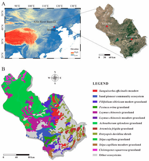
Figure 1.
(A): Location of the Xilin River Basin (XRB); (B): distribution of twelve ecosystems in the XRB. The base maps of A on the left and right are from Diva-GIS (www.diva-gis.org) and Google Earth respectively.
2.2. Data
2.2.1. Ecosystem Classification Data
Land cover data and vegetation data were obtained from the Ministry of Ecology and Environment Centre for Satellite Application on Ecology and Environment (China) (http://www.secmep.cn). Thirteen land cover types were classified based on the land cover classification system (LCCS) defined by the Food and Agriculture Organization of the United Nations (FAO). To determine the precision of the RS interpretation, the classification results were assessed via Kappa coefficients. The Kappa coefficients for 2000 and 2015 are 86.03% and 83.55%.
In this study, we assessed the ecosystem at the genus level. According to the Database for Ecosystems and Ecosystem Services Zoning in China, each ecosystem genus is determined by constructive species (co-constructive species) [32]. We named ecosystems with its constructive species: Ostryopsis davidiana shrub, Sanguisorba officinalis meadow, Stipa capillata grassland, Artemisia frigida grassland, Cleistogenes squarrosa grassland, Leymus chinensis grassland, Achnatherum splendens grassland, sandy pioneer plant communities (grassland), Festuca ovina grassland, Leymus chinensis meadow grassland, Stipa capillata meadow grassland, and Spiraea salicifolia shrub (Figure 1B). Twelve ecosystems were grouped into nine ecosystem families and three ecosystem orders based on the IUCN Habitats Classification Scheme 3.0 in combination with Database for Ecosystems and Ecosystem Services Zoning in China [32]. These twelve dominant ecosystems, occupying more than 70% of the area were selected as the assessment targets.
2.2.2. Other Data
Leaf area index (LAI), normalized difference vegetation index (NDVI), meteorological, and soil data were used in the BEPS to develop the indicators for evaluating ecosystem status. We utilized the MOD13A1 and MOD15A2 16-day NDVI product and LAI product at a 500-m spatial resolution in 2000 and 2015, respectively (derived from EOS/MODIS of NASA) [33]. We applied the MODIS Reprojection Tools (the National Center for Supercomputing Applications, Chicago, US) to covert downloaded MODIS-NDVI and MODIS-LAI from HDF to TIFF and re-project output data to WGS84. Monthly MODIS-NDVI and monthly MODIS-LAI were obtained from 16-day NDVI product and 16-day LAI product based on maximum value composite (MVC) in ArcGIS (Esri, California, US). The XRB zoning map was used to extract the monthly NDVI and LAI grids in the region from 2000 to 2015. The meteorological data, including the average monthly temperature, monthly precipitation, monthly net radiation, and monthly mean relative humidity during 2000~2015, were collected from the Chinese Meteorological Data Sharing Service Network [34]. Data on the available water-holding capacity of soil were compiled in a GIS soil database at the geographical information monitoring cloud platform [35].
2.3. Methods
2.3.1. Ecosystem Assessment System
According to the IUCN criteria, ecosystems were classified into eight categories. Initially, all ecosystems are considered not evaluated (NE). Ecosystems should be evaluated using all criteria. If the data for all criteria are unavailable, the ecosystem should be classified as data deficient (DD). Once data are available, the status of an ecosystem is assigned to one of the remaining six categories based on the criteria and threshold: least concern (LC), near threatened (NT), vulnerable (VU), endangered (EN), critically endangered (CR), and collapsed (CO). The assessment was conducted at the ecosystem level instead of the single-species level, which is consistent with other the IUCN RLE-based studies.
- The absolute rate of decline
According to the Guidelines for the Application of IUCN Red List of Ecosystems Categories and Criteria, the time frames of assessment (under criteria A, C, and D) include the past 50 years, any 50 years and since 1750 [36]. Because of the data deficiency, assessments of changes in the past were not conducted. Assessment of future changes was based on the predictions of changes over any 50 years. Two scenarios including the proportional rate of decline (PRD) and the absolute rate of decline (ARD) were proposed to predict the future changes. Here we assume that variables decrease linearly every year. This model might introduce uncertainty, more efforts are needed to generate a more realistic model. We made predictions of changes for any 50 years (2000–2050) based on ARD over 15 years. A 15-year interval is common in the IUCN RLE-based grassland studies [2]. It is consistent with official guidelines for the RLE as well. The Guidelines for the Application of IUCN Red List of Ecosystems Categories and Criteria 2.0 provides an example study using 1986–2001 to first estimate an observed rate of change over 15 years, and then extrapolating projected losses to 2036 [36]. Given the above-mentioned reasons, we consider the time interval here is appropriate. The change in the ecosystems from 2000 to 2050 can be predicted from Equation (1):
where is the value at year and is the value at year . In the present study, the temporal scale is 15 years from 2000 to 2015. R is a proportion of change (%).
- Criterion A: reduction in geographic distribution
Criterion A is to identify ecosystems that are undergoing a decline in areas that influences the risk of collapse [5]. In this study, we evaluated the threat status of ecosystems under subcriterion A2 (reduction over any 50 years) by calculating the area they occupied. Future change assessment was based on the prediction of changes of geographical distribution from 2000 to 2050 calculated by the equation (1).
- Criterion B: restricted geographic distribution
The primary role of criterion B is to identify ecosystems whose distributions are restricted to the extent, facing the risk of collapse under threatening events or processes [37]. Criterion B was used to assess restricted distribution in terms of the extent of occurrence (EOO) (B1), the area of occupancy (AOO) (B2), and the number of locations (served as B3 here). The EOO was estimated using a minimum convex polygon enclosing all the sites within an ecosystem type. The AOO was calculated by counting the number of 10 × 10 km grains within the EOO covered by an ecosystem.
- Criterion C: environmental degradation
Criterion C evaluates the risk of ecosystem collapse caused by the degradation of the abiotic environment [38]. It was used to assess environmental degradation over the past 50 years (C1), any 50 years (C2), and since 1750 (C3) based on the changes in abiotic variables. In the analysis, soil water deficit (SWD) and soil carbon (SC) were selected as environmental indicators to assess environmental degradation. SWD and SC in 2050 were calculated by the Equation (1). Regarding the guidelines, the key to assessing criteria C and D is relative severity. It is because relative severity is essential for comparing risks among ecosystems suffering from different degradation [36]. In this study, the values of parameters in 2000 are regarded as the initial values and collapse value is assumed to be zero. The relative severity of decline is calculated as
where the parameter in 2000 and represents the parameter in 2050.
- Criterion D: disruption of biotic processes and interactions
Criterion D considers the extent of the ecosystem that is subjected to the disruption of biotic processes and the severity of disruption [39]. Here, the dimidiate pixel model and BEPS were applied to simulate biological processes and construct biological indicators. Vegetation fractional coverage (VFC), vegetation evaporation (EV), net primary production (NPP), belowground net primary production (BNPP), aboveground net primary production (ANPP), gross primary production (GPP), and net ecosystem production (NEP) are selected to represent the biological process. The change of these seven indicators from 2000 to 2050 is calculated by the Equation (1). The relative severity of decline was calculated by the Equation (2) as well. In this contribution, we only focus on the dynamics of vegetation. We realize that ecosystems have multiple components and fauna is important as well. Yet it is still challenging not only for our study but for other studies [21]. Fauna is highly movable and it is difficult to track them every year and make predictions for several decades. Besides, interactions between fauna and flora are complicated, and it might cause more uncertainties for assessment if we could not tackle this issue properly. More importantly, since quantification and assessment of fauna indicators for the RLE have not had consistency so far, it is hard to assess them [36]. More efforts will be needed to improve the assessment of biotic processes and interactions.
- Determining the threat level
For criteria C and D, we calculated the relative severity of the decline. Then we categorized relative severity (≥30%) into three degrees: ≥80% (d1), ≥50% (d2), and ≥30% (d3). Different relative severity degrees were combined with a proportion of area they occupied to assign threat levels for twelve ecosystems. Table 1 is an overview of sub-criteria and thresholds adopted in this study. Following the precautionary principle, the overall risk status of the ecosystem will be the highest risk category obtained by any of the assessed criteria.

Table 1.
Subcriteria and thresholds applied in this study.
2.3.2. Boreal Ecosystem Productivity Simulator (BEPS)
Process-based biogeochemical models can integrate the input data, automate the modeling, and produce the output of ecological parameters. It has been a useful tool for revealing mechanisms of biological process and plant–environment interaction. BEPS is a more reliable process model than others in terms of availability and quality of required data and accuracy of simulation results. Accuracy of BEPS simulation is estimated 60% for single pixel (1 km2) and 75% for 3 × 3 pixels (9 km2) [40]. In this study, nine indicators were developed based on the BEPS to assess environmental degradation and the decline of biotic processes (Table 2). More details about BPES can be found in the reference paper. To evaluate the accuracy of model results, we compared the NPPs of Stipa capillata grassland and Festuca ovina grassland obtained from ground measurements with those obtained from the BEPS. In 2015, for Stipa capillata grassland, the R2 value of the relationship between observed and modeled NPP was 0.725, whereas that of Festuca ovina grassland was 0.603. According to the previous studies [41,42,43,44], the modeled results are appropriate for use in an ecosystem assessment system. An overview of the conceptual framework is shown in Figure 2.
Table 2.
Outputs of boreal ecosystem productivity simulator (BEPS) selected as parameters for criteria C and D.
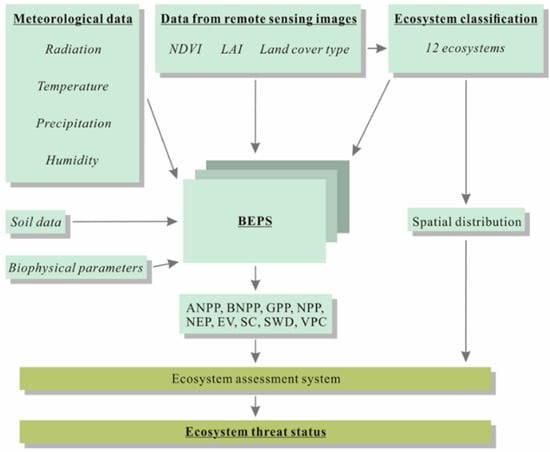
Figure 2.
The conceptual framework showing inputs/outputs data of BEPS and spatial data serve as inputs data for the assessment of ecosystems.
3. Results
3.1. Criterion A, Reduction in Geographic Distribution
Reduction from 2000 to 2050 (A2)
From 2000 to 2015, the total area had decreased by 0.5%. Stipa capillata grassland occupied the greatest area, and from 2000 to 2015, it experienced the most noticeable decrease of 93.4 km2. Artemisia frigida grassland accounted for the smallest proportion of the total area. From 2000 to 2050, Stipa capillata grassland, Achnatherum splendens grassland, and sand pioneer plant community ecosystems were simulated to decrease by 41.22%, 40.01%, and 42.54%, respectively, while the remaining ecosystems experienced slight increases (Figure 3). According to sub-criterion A2 (decrease > 30%), Stipa capillata grassland, Achnatherum splendens grassland, and sand pioneer plant community ecosystems were assigned to the VU category, whereas the other nine ecosystems were assigned to LC. Because of the lack of data necessary to evaluate the geographic changes over the past 50 years and since 1750, the status of all twelve ecosystems under criteria A1 and A3 are listed as DD.
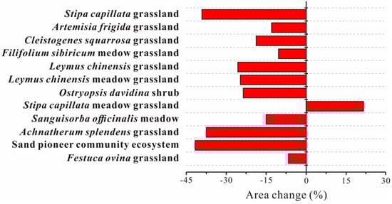
Figure 3.
Simulated change of areas of twelve ecosystems from 2000 to 2050.
3.2. Criterion B, Restricted Geographic Distribution
3.2.1. EOO (B1)
Stipa capillata grassland was the most widely distributed ecosystem type, covering an area of 31,154 km2, whereas Festuca ovina grassland was the most limited type (Table 3, Figure 4). Artemisia frigida grassland, Cleistogenes squarrosa grassland, Ostryopsis davidina shrub, Sanguisorba officinalis meadow grassland, sand pioneer community ecosystem, and Festuca ovina grassland each occupied less than 10,000 km2; and according to sub-criterion B1, they all have VU status. The remaining ecosystems were assigned into LC.
Table 3.
Restricted distribution of twelve ecosystems.
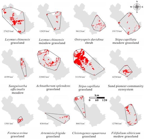
Figure 4.
Restricted distribution of twelve ecosystems in the XRB in 2015.
3.2.2. AOO (B2)
The area occupied by the ecosystems was at 10 × 10 km grain size, and those occupying less than 1 km2 were excluded as Figure 5 shows. Analogous to the geographic distributions, Stipa capillata grassland accounted for the largest number, with 178 grid cells, whereas Festuca ovina grassland accounted for the smallest number, with only nine grid cells. According to the evaluation sub-criterion B2, Festuca ovina grassland, which occupied fewer than 20 grid cells, belongs to the EN category. Artemisia frigida grassland, Cleistogenes squarrosa grassland, Leymus chinensis meadow grassland, Sanguisorba officinalis meadow grassland, and sand pioneer community ecosystem occupied less than 50 grid cells and were assigned to the VU category. The remaining ecosystems belonged to the LC category.
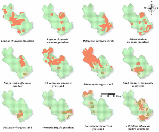
Figure 5.
Grids of distribution of different ecosystems in the XRB in 2015. The orange cells represent ecosystems under the measurement of B2.
3.2.3. Number of Locations (B3)
According to the sub-criterion B3, easily affected locations of each ecosystem were counted. Festuca ovina grassland had less than five locations, and it belonged to the EN category. Artemisia frigida grassland, Sanguisorba officinalis meadow grassland, and sand pioneer community ecosystem occupied less than ten locations; thus, these ecosystems belonged to the VU category. The remaining ecosystems belonged to the LC category.
3.3. Criterion C, Environmental Degradation
Environmental Degradation from 2000 to 2050 (C2)
From 2000 to 2050, none of the ecosystems showed noticeable declines in SWD and SC, and areas with decreasing trends in environment quality accounted for less than 1% of the total (Figure 6 and Figure 7). According to sub-criterion C2, twelve ecosystems were assessed as LC. C1 and C3 are not assessable because of data deficiency.
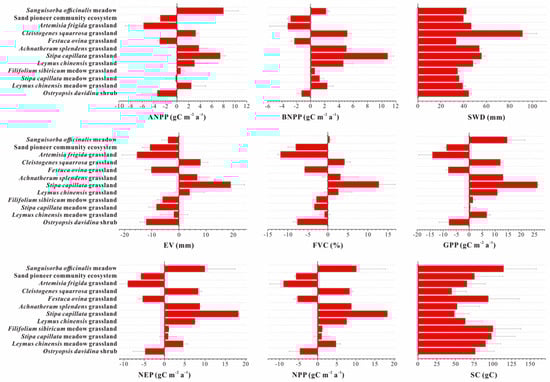
Figure 6.
Change of environment status (SWD, SC) and biological process (ANPP, BNPP, EV, FVC, GPP, NEP, and NPP) for twelve ecosystems from 2000 to 2015.
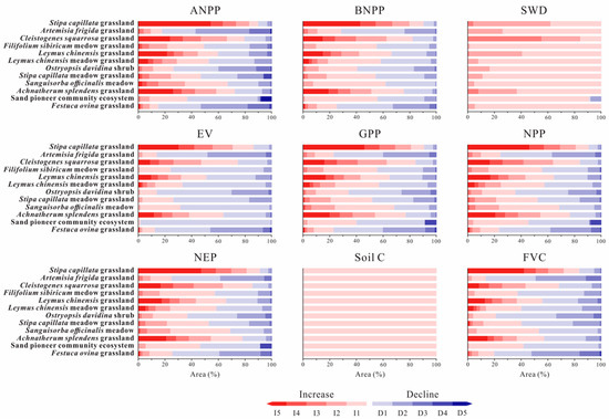
Figure 7.
The fraction of extent of twelve ecosystems affected by the change of environment status (SWD, SC) and biological process (ANPP, BNPP, EV, FVC, GPP, NEP, and NPP) from 2000 to 2050. (decline = D, increase = I): D1 (0–20%), D2 (20–40%), D3 (40–60%), D4 (60–80%), D5 (80–100%), I1 (0–20%), I2 (20–40%), I3 (40–60%), I4 (60–80%), I5 (80–100%).
3.4. Criterion D, Disruption of Biotic Processes and Interactions
Disruption of Biotic Process and Interactions from 2000 to 2050 (D2)
The biotic interactions and biological processes were quantitatively assessed by ANPP, BNPP, GPP, NPP, NEP, EV, and VFC. Total of 93.45% of Artemisia frigida grassland and 52.36% of Festuca ovina grassland were assigned into d2 and d1 respectively. Ostryopsis davidina shrub in d3 and Stipa capillata meadow grassland in d2 accounted for 81.15% and 35.44% respectively. According to sub-criterion D2, Artemisia frigida grassland and Festuca ovina grassland were at the EN level. Ostryopsis davidina shrub and Stipa capillata meadow grassland were at the VU level. D1 and D3 are not assessable because of data deficiency.
3.5. Assessment Result of Twelve Ecosystems
Based on RLE, we assigned the threat levels to the twelve ecosystems in the XRB. As Table 4 shows, Artemisia frigida grassland and Festuca ovina grassland faced EN-level threat; Filifolium sibiricum meadow grassland and Leymus chinensis grassland had LC status; and the remaining are at the VU level, which was the most common.
Table 4.
The threat level of all twelve ecosystems in the XRB. Following the precautionary principle, the highest risk category obtained by any of the assessed criteria will be the overall risk status of the ecosystem.
Different ecosystems faced different threats caused by various factors (Figure 8). Artemisia frigida grassland and Festuca ovina grassland faced the highest risks of collapse because of the declines in restricted distribution and environmental quality. Compared with Artemisia frigida grassland, Festuca ovina grassland experienced a more severe decline in restricted distribution. Achnatherum splendens grassland and Stipa capillata grassland were identified to be vulnerable resulting from the degradation in geographic distribution, whereas Leymus chinensis meadow grassland, Sanguisorba officinalis meadow, and Cleistogenes squarrosa grassland were identified as vulnerable because of the declines in restricted distribution and degradation. Ostryopsis davidina shrub and Stipa capillata meadow grassland suffered from the degradation because of environmental quality decline, whereas sand pioneer community ecosystem faced threat caused by declines in geographic distribution and restricted distribution. Thus, to conserve the different ecosystems, different measures should be taken. For example, for Artemisia frigida grassland and Festuca ovina grassland, measures on conservation of habitat can be taken.
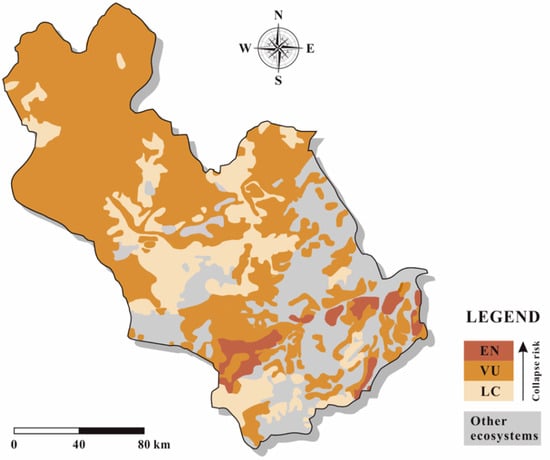
Figure 8.
The extent of the threat status of biodiversity in the study area.
4. Discussion
4.1. Implications and Limitations
Twelve selected local ecosystem genera were evaluated by the IUCN RLE in combination with GIS, RS, and BEPS. According to Keith et al. (2015), RLE-based ecosystem assessments should be judged by whether it achieves conservation and management ends, whether its limitations can be compensated by its advantages and benefit, and whether it performs better than alternative methods [45]. In this study, the threat status of each ecosystem was tracked and threat levels were assigned to each ecosystem systematically. It will promote its current and potential applications in legislation, policy, environmental management, and education in China. Besides, it can be more widely used and efficient than other current assessments in China. Considering these aspects, we think our ecosystem-centered study is appropriate. In addition, results are consistent with the previous studies, indicating that the status of multiple ecosystems in Inner Mongolia can be assessed by the RLE [5,36,37,38,39]. It demonstrates the feasibility and possibility of applying the IUCN RLE in China. It also proves that data deficiency can be overcome to some extent by introducing the BEPS. BEPS as a virtual lab allows us to get biological indicators of vegetation and environment with high accuracy. It can be improved as knowledge, data availability, and quality improve [46]. BEPS can be adjusted and applied with higher accuracy in the future study.
However, there are potential limitations in this study. The persistence of biota within an ecosystem relies on biotic processes and interaction. These include predatory, species invasions, and trophic and pathogenic processes, et cetera. Diversity of organisms and process are important. Significant disruptions in process and interactions can even cause a collapse of the ecosystem [1,36]. However, in this study, our results only depend on the biological process and dynamics of vegetation. Other important elements in the ecosystem such as animal activities, trophic diversity, a spatial flux of organisms, interaction diversity are not taken into account. Though our assessment performs well, more effort in selecting biodiversity indicators and presenting complicity of the ecosystem is needed. Besides, the assessment still has uncertainties in spatial and functional symptoms [36]. Possible errors in mapping and classification can result in biased distribution. Because of the lack of data, we failed to calculate the past decline to distinguish directional change. For the future, study about reducing assessment errors and developing a more comprehensive model is necessary.
4.2. Future Predictions and Conservation Strategy for Local Ecosystems
In the XRB, Artemisia frigida grassland and Festuca ovina grassland face the highest threat level, EN, because of declines in biological processes and restricted distribution. If the trend persists, Artemisia frigida grassland and Festuca ovina grassland will be at the risk of collapse in the future. Other ecosystems with VU classification face survival challenges from geographic and restricted distribution. They would face higher levels of threats unless effective ecological management programs are implemented.
In the past decades of the XRB, the irregularity of patches and the degree of fragmentation have increased, with the area of dominant patches and patch connectivity decreasing [47,48]. Landscape alteration in the XRB is detrimental to ecosystem growth since it limits species immigration and emigration, which further affects the predictor–prey network and leads to the gene pool and biodiversity loss. Land use considered the main driver of landscape change should be managed properly. According to the previous studies, during the past decades, the area of grassland has decreased with city expansion, farmland reclamation, and mine exploration in Xilin Hot. Besides, mines in Xilin Hot are concentrated in grassland in the XRB, which increase local habitat fragmentation [49]. Control of the intensity of mining, allocation of mining spots, and management of the human landscape are important for conserving local ecosystems. Establishing the protected areas and land use management system is beneficial for protecting ecosystems against degradation. The ANPP of degraded ecosystems increased by 69% and vegetation cover increased by 45% after the areas were fenced [30].
4.3. Biodiversity Conservation Based on the IUCN RLE in China
Though the RLE can be used in the study area, there are some potential limitations in applying it widely. To improve the assessment and promote the application of the IUCN RLE in China, additional progress is needed. Except for variables mentioned in this study, a broad set of variables that are potentially useful for quantifying biotic processes and associated functional declines could be further considered. These could include changes in species richness, composition, and dominance; relative abundance of species functional types, guilds or alien species; measures of interaction diversity; measures of niche diversity and structural complexity [36]. For example, in China, by 2003, the number of invasive species reached 283, and invasive organisms can threaten local ecosystems through range expansion [50,51]. Thus, the system of ecosystem assessment could take a relative abundance of alien species into consideration to identify the major threats to local systems in regions suffering bio-invasion. Furthermore, there are inconsistencies between Chinese nature reserve classification and IUCN protected area categories in classification standards, management targets and functions [52]. To maximize the accuracy of comprehensive assessment, the adjustment of nature reserve classification to better correspond with IUCN protected area classification could be taken into accounts.
According to the China National Biodiversity Conservation Strategy and Action Plan (2011–2030), major challenges in biodiversity conservation include a lack of monitoring systems for biodiversity and limited awareness of biodiversity conservation [14]. The reasonable application of IUCN RLE can be of benefit to address these two major issues to some extent. The criteria are easily quantified and used, and they can directly reflect the status and changes of ecosystems. They will help establish a dynamic monitoring network for ecosystems in China [22]. Also, ecosystems whose services and functions are closely correlated with human beings are important for human wellbeing, and ecosystem assessment results can serve as a good educational tool to raise public awareness of biodiversity conservation [53]. The IUCN RLE can also contribute to the design of protected areas, smart city, natural resource management strategies, and frameworks for sustainable development [54].
5. Conclusions
In this study, we assessed the threat level of twelve dominant ecosystems on the base of IUCN RLE in the XRB by integrating the tools of geographical information systems, remote sensing, and boreal ecosystem productivity simulator. The integrated tools overcome the limits of data deficiency and increase the efficiency of the IUCN RLE to some extent. The results indicate that Artemisia frigida grassland and Festuca ovina grassland are facing EN-level threat; Filifolium sibiricum meadow grassland and Leymus chinensis grassland are at LC-level threatened status, and the remaining eight ecosystems are at VU-level threatened status. Artemisia frigida grassland and Festuca ovina grassland will be at the risk of collapse if this trend maintains. According to assessment results, conservation of habitat and land management are proposed for local biodiversity conservation. Although there are potential uncertainties and limitations, our preliminary results are consistent with previous studies. It demonstrates the applicational feasibility of the IUCN RLE in China and possibility of combining the IUCN RLE with the model. Our study will shed light on the future study, protection, and restoration of the XRB and further application of the IUCN RLE in China. For future studies, with the development of real-time tracking and computing, more aspects of the ecosystem will be explored and presented. The coverage of the IUCN RLE will be expanded and it will be possible to report biodiversity at the global level.
Author Contributions
Conceptualization, K.Z.; formal analysis, X.M., D.W., and R.H.; funding acquisition, L.G.; methodology, K.Z.; supervision, L.G.; visualization, H.H. and X.M.; writing of original draft and revisions, X.M., H.H., and L.G. All authors have read and agreed to the published version of the manuscript.
Funding
This study was funded by the National Key R&D Program of China FUNDER, grant number 2017YFC0505601 and innovation team project of Chinese Nationalities Affairs Commission (10301-0190040129).
Acknowledgments
We acknowledge the constructive comments of the three anonymous reviewers.
Conflicts of Interest
The authors declare no conflict of interest.
References
- Rodríguez, J.P.; Rodríguez-Clark, K.M.; Baillie, J.E.; Ash, N.; Benson, J.; Boucher, T.; Brown, C.; Burgess, N.D.; Collen, B.E.; Jennings, M.; et al. Establishing IUCN red list criteria for threatened ecosystems. Conserv. Biol. 2011, 25, 21–29. [Google Scholar] [CrossRef] [PubMed]
- Rodríguez, J.P.; Balch, J.K.; Rodríguez-Clark, K.M. Assessing extinction risk in the absence of species-level data: Quantitative criteria for terrestrial ecosystems. Conserv. Biol. 2007, 16, 183–209. [Google Scholar] [CrossRef]
- Bradley, B.A. Assessing ecosystem threats from global and regional change: Hierarchical modeling of risk to sagebrush ecosystems from climate change, land use and invasive species in Nevada, USA. Ecography 2010, 33, 198–208. [Google Scholar] [CrossRef]
- Barrett, S.; Yates, C.J. Risks to a mountain summit ecosystem with endemic biota in southwestern Australia. Austral Ecol. 2015, 40, 423–432. [Google Scholar] [CrossRef]
- Williams, R.J.; Wahren, C.H.; Stott, K.A.J.; Camac, J.S.; White, M.; Burns, E.; Harris, S.; Nash, M.; Morgan, J.W.; Venn, S.; et al. An International Union for the Conservation of Nature Red List ecosystems risk assessment for alpine snow patch herb fields, South-Eastern Australia. Austral Ecol. 2015, 40, 433–443. [Google Scholar] [CrossRef]
- Wardle, G.M.; Greenville, A.C.; Frank, A.S.; Tischler, M.; Emery, N.J.; Dickman, C.R. Ecosystem risk assessment of Georgina gidgee woodlands in central Australia. Austral Ecol. 2015, 40, 444–459. [Google Scholar] [CrossRef]
- Tozer, M.G.; Leishman, M.R.; Auld, T.D. Ecosystem risk assessment for Cumberland Plain Woodland, New South Wales, Australia. Austral Ecol. 2015, 40, 400–410. [Google Scholar] [CrossRef]
- International Union for Conservation of Nature and Natural Resources (IUCN). Available online: http://www.iucnredlistofecosystems.org/resources/outreach/progress-rle-2014%E2%80%9015/ (accessed on 2 March 2016).
- Bland, L.M.; Nicholson, E.; Miller, R.M.; Andrade, A.; Carré, A.; Etter, A.; Ferrer-Paris, J.R.; Herrera, B.; Kontula, T.; Lindgaard, A.; et al. Impacts of the IUCN Red List of Ecosystems on conservation policy and practice. Conserv. Lett. 2019, 12, e12666. [Google Scholar] [CrossRef]
- Lytras, M.D.; Visvizi, A.; Sarirete, A. Clustering smart city services: Perceptions, expectations, responses. Sustainability 2019, 11, 1669. [Google Scholar] [CrossRef]
- Visvizi, A.; Lytras, M.D. Smart Cities: Issues and Challenges: Mapping Political, Social and Economic Risks and Threats; Elsevier: Amsterdam, The Netherlands, 2019; pp. 350–372. [Google Scholar]
- Visvizi, A.; Lytras, M.D.; Mudri, G. Smart Villages in the EU and Beyond; Emerald Publishing: Bingley, UK, 2019; pp. 20–27. [Google Scholar]
- Liu, J.; Chen, J.M.; Cihlar, J.; Park, W.M. A process-based boreal ecosystem productivity simulator using remote sensing inputs. Remote Sens. Environ. 1997, 62, 158–175. [Google Scholar] [CrossRef]
- Ministry of Environmental Protection of the People’s Republic of China (MEPPRC). China National Biodiversity Conservation Strategy and Action Plan (2011–2030); Biodiversity Office: Beijing, China, 2010. [Google Scholar]
- Ma, J. Ecosystem Assessment of Ebinur Watershed Natural Reserve. Sci. Technol. Innov. Her. 2013, 8, 46–47. [Google Scholar]
- Xiao, J.M.; Yang, S.Y. Application of the PSR Model to the Assessment of Island Ecosystem. J. Xiamen Uni. (Nat. Sci.) 2007, 46(z1), 191–196. [Google Scholar] [CrossRef]
- Di, B.F.; Yang, Z.; Ai, N. Evaluation on Degraded Ecosystem in Jinshajiang Xerothermic Valley Using RS and GIS-A Case Study of Yuanmou County in Yunnan. Sci. Geogr. Sin. 2005, 25, 450–484. [Google Scholar]
- Cai, K.; Qin, C.Y.; Li, J.Y.; Zhang, Y.; Niu, Z.C.; Li, X.W. Preliminary study on phytoplanktonic index of biotic integrity (P-IBI) assessment for lake ecosystem health: A case of Taihu Lake in Winter. Acta Ecol. Sin. 2012, 36, 1431–1441. [Google Scholar]
- Yan, Z.C.C.S.L.; Jie, L.Q.J.X.D. Ecosystem Assessment of Xarxili Natural Reserve in Xinjiang. Sci. Technol. Innov. Her. 2013, 146–149. [Google Scholar] [CrossRef]
- Tan, J.; Li, A.; Lei, G. Establish IUCN Red List of ecosystems in Southwestern China based on remote sensing data. In Proceedings of the IEEE International Geoscience and Remote Sensing Symposium (IGARSS), Beijing, China, 10–15 July 2016; pp. 1307–1310. [Google Scholar]
- Tan, J.; Li, A.; Lei, G.; Bian, J.; Chen, G.; Ma, K. Preliminary assessment of ecosystem risk based on IUCN criteria in a hierarchy of spatial domains: A case study in Southwestern China. Biol. Conserv. 2017, 215, 152–161. [Google Scholar] [CrossRef]
- Zhu, C.; Fang, Y.; Zhou, K.X.; Mu, S.J.; Jiang, J.L. IUCN Red List of Ecosystems, a new tool for biodiversity conservation. Acta Ecol. Sin. 2015, 35, 2826–2836. [Google Scholar]
- He, C.; Tian, J.; Gao, B.; Zhao, Y. Differentiating climate-and human-induced drivers of grassland degradation. in the Liao River Basin, China. Environ. Monit. Assess. 2015, 187, 4199. [Google Scholar] [CrossRef]
- Ren, H.; Zheng, S.; Bai, Y. Effects of grazing on foliage biomass allocation of grassland communities in XRB, Inner Mongolia. J. Plant Ecol. (Chin. Ver.) 2009, 33, 1065–1074. [Google Scholar]
- Tong, C.; Yong, W.; Wu, Y.; Zhao, L.; Jiang, C.; Yong, S. Change in the spatial structure of grassland vegetation in the XRB from 1985 to 1999. Acta Sci. Nat. Uni. NeiMonggol (Nat. Sci. Ed.) 2001, 3, 562–566. [Google Scholar]
- Han, Y.; Niu, J.; Zhang, Q.; Dong, J.; Zhang, X.; Kang, S. The changing of vegetation pattern and its driven forces of grassland in XRB in thirty years. Chin. J. Grassl. 2014, 36, 70–77. [Google Scholar]
- Zhang, X.; Niu, J.; Buyantuev, A.; Zhang, Q.; Dong, J.; Kang, S.; Zhang, J. Understanding grassland degradation and restoration from the perspective of ecosystem services: A case study of the XRB in Inner Mongolia, china. Sustainability 2016, 8, 594. [Google Scholar] [CrossRef]
- Chen, S.; Liu, J.; Zhuang, D.; Xiao, X.M.; Boles, S. Quantifying land use and land cover change in XRB using multi-temporal Landsat TM/ETM sensor data. Acta Geogr. Sin. Chin. Ed. 2003, 58, 45–52. [Google Scholar]
- Zhang, X.; Niu, J.; Zhang, Q.; Dong, J.; Zhang, J. Soil conservation function and its spatial distribution of grassland ecosystems in XRB, Inner Mongolia. Acta Pratacultuae Sinica 2005, 24, 12–20. [Google Scholar]
- Xi, X.K.; Zhu, Z.; Hao, X. Grassland Plant Communities Classification and Diversity Analysis in the XRB. Ecol. Environ. Sci. 2016, 25, 1320–1326. [Google Scholar]
- Hao, R.; He, J.L.; Dan, S.; Liu, Y.P.; Liang, Z.Q. Effects of vegetation restoration methods on soil and water conservation of degraded grassland in Xilinhe River watershed. Grassl. Turf. 2016, 36, 52–57. [Google Scholar] [CrossRef]
- IUCN Habitats Classification Scheme Version 3. Available online: http://www.iucnredlist.org/technical-documents/classification-schemes/habitats-classification-scheme-ver3 (accessed on 25 May 2016).
- EOS/MODIS of NASA. Available online: http://edcimswww.cr.usgs.gov/pub/imswelcome/ (accessed on 23 April 2016).
- Chinese Meteorological Data Sharing Service Network. Available online: http://cdc.cma.gov.cn (accessed on 25 June 2016).
- Geographical Information Monitoring Cloud Platform. Available online: www.dsac.cn (accessed on 27 August 2016).
- Bland, L.M.; Keith, D.A.; Miller, R.M.; Murray, N.J.; Rodríguez, J.P. Guidelines for the Application of IUCN Red List of Ecosystems Categories and Criteria, Version 1.1; International Union for the Conservation of Nature: Gland, Switzerland, 2017. [Google Scholar]
- Auld, T.D.; Leishman, M.R. Ecosystem risk assessment for Gnarled Mossy Cloud Forest, Lord Howe Island, Australia. Austral Ecol. 2015, 40, 364–372. [Google Scholar] [CrossRef]
- Rodríguez, J.P.; Keith, D.A.; Rodríguez-Clark, K.M.; Murray, N.J.; Nicholson, E.; Regan, T.J.; Miller, R.M.; Barrow, E.G.; Bland, L.M.; Boe, K.; et al. A practical guide to the application of the IUCN Red List of Ecosystems criteria. Philos. Trans. Royal Soc. B Biol. Sci. 2015, 370, 20140003. [Google Scholar] [CrossRef]
- Lal, R. Soil carbon sequestration impacts on global climate change and food security. Science 2004, 304, 1623–1627. [Google Scholar] [CrossRef]
- Cui, B.; Yang, Q.; Yang, Z.; Zhang, K. Evaluating the ecological performance of wetland restoration in the Yellow River Delta, China. Ecol. Eng. 2009, 35, 1090–1103. [Google Scholar] [CrossRef]
- Zhang, F.; Tiyip, T.; Ding, J.; Sawut, M.; Johnson, V.C.; Tashpolat, N.; Gui, D. Vegetation fractional coverage change in a typical oasis region in Tarim River Watershed based on remote sensing. J. Arid Land 2013, 5, 89–101. [Google Scholar] [CrossRef]
- Davidson, E.A.; Verchot, L.V.; Cattanio, J.H.; Ackerman, I.L.; Carvalho, J.E.M. Effects of soil water content on soil respiration in forests and cattle pastures of eastern Amazonia. Biogeochemistry 2000, 48, 53–69. [Google Scholar] [CrossRef]
- Liu, Z.; Zhou, Y.; Ju, W.; Gao, P. Simulation of soil water content in farm lands with the BEPS ecological model. Trans. Chin. Soc. Agric. Eng. 2011, 27, 67–72. [Google Scholar]
- Lu, W.; Fan, W.Y.; Tian, T. Parameter optimization of BEPS model based on the flux data of the temperate deciduous broad-leaved forest in Northeast China. J. Appl. Ecol. 2016, 27, 1353–1358. [Google Scholar]
- Keith, D.A.; Rodríguez, J.P.; Brooks, T.M.; Burgman, M.A.; Barrow, E.G.; Bland, L.; Comer, P.J.; Franklin, J.; Link, J.; McCarthy, M.A.; et al. The IUCN red list of ecosystems: Motivations, challenges, and applications. Conserv. Lett. 2015, 8, 214–226. [Google Scholar] [CrossRef]
- Wang, X.X.; Sun, T.; Zhu, Q.J.; Liu, X.; Chen, S.H. Spatio-temporal variation of net primary productivity estimated with BEPS model in the urban area. J. Arid Land Resour. Environ. 2014, 28, 1–5. [Google Scholar] [CrossRef]
- Liu, H.L.; Xu, X.M.; Jiao, R.; Liang, W.T. 2016. Relationship between annual precipitation and vegetation cover in the XRB. Sci-tech Paper 2016, 9, 289–290. [Google Scholar]
- Sulungaowa, B.; Suya, B. Influence of Climatic Variation on the Evolution of Landscape Pattern of XRB. Meteor. J. Inn. Mong. 2015, 23–27. [Google Scholar]
- Tong, C.; Xi, F.J.; Yang, J.R.; Yong, W.Y.; Zhang, P.; Yong, S.P. Remote sensing monitoring on degraded steppe and determination of reasonable grazing intensity for the restoration of steppe in middle reach of Xilin river basin. Acta Pratacult. Sin. 2003, 12, 78–83. [Google Scholar]
- Keith, D.A.; Rodriguez, J.P.; Barrow, E.G. A framework for monitoring the status of Australia’s ecosystems based on IUCN’s new global standard. In Valuing Nature: Protected Areas and Ecosystem Services; Australian Committee for IUCN Inc.: Sydney, Australia, 2015; pp. 62–68. Available online: www.aciucn.org.au (accessed on 3 February 2020).
- Zheng, Y.Q.; Zhang, C.H. Current status and progress of studies in biological invasion of exotic trees. Sci. Silvae Sin. 2006, 42, 114–122. [Google Scholar]
- Wang, Z.; Jiang, M.K.; Zhu, G.Q.; Tao, S.M.; Zhou, H.L. Comparison of Chinese nature reserve classification with IUCN protected area categories. Rural Eco-Environ. 2004, 20, 72–76. [Google Scholar]
- Murray, N.J.; Ma, Z.; Fuller, R.A. Tidal flats of the Yellow Sea: A review of ecosystem status and anthropogenic threats. Austral Ecol. 2015, 40, 472–481. [Google Scholar] [CrossRef]
- Visvizi, A.; Lytras, M.D. Smart cities research and debate: What is in there? In Smart Cities: Issues and Challenges: Mapping Political, Social and Economic Risks and Threats; Elsevier: Amsterdam, The Netherlands, 2019; pp. 1–14. [Google Scholar]
© 2020 by the authors. Licensee MDPI, Basel, Switzerland. This article is an open access article distributed under the terms and conditions of the Creative Commons Attribution (CC BY) license (http://creativecommons.org/licenses/by/4.0/).