Multi-Period Generation Expansion Planning for Sustainable Power Systems to Maximize the Utilization of Renewable Energy Sources

Abstract

The increasing penetration of renewable energy brings great challenges to the planning and operation of power systems. To deal with the fluctuation of renewable energy, the main focus of current research is on incorporating the detailed operation constraints into generation expansion planning (GEP) models. In most studies, the traditional objective function of GEP is to minimize the total cost (including the investment and operation cost). However, in power systems with high penetration of renewable energy, more attention has been paid to increasing the utilization of renewable energy and reducing the renewable energy curtailment. Different from the traditional objective function, this paper proposes a new objective function to maximize the accommodation of renewable energy during the planning horizon, taking into account short-term operation constraints and uncertainties from load and renewable energy sources. A power grid of one province in China is modified as a case study to verify the rationality and effectiveness of the proposed model. Numerical results show that the proposed GEP model could install more renewable power plants and improve the accommodation of renewable energy compared to the traditional GEP model.

1. Introduction

Generation expansion planning (GEP), which has been studied continuously in recent decades, plays a critical role in the power sector and sustainable energy development [1,2]. It mainly aims to acquire an optimal generation mix by determining the time, location, size, and type of different candidate generating facilities to meet the future load demand, guaranteeing that the power system stays reliable and secure [3]. With the planning horizon varying from several years to several decades, GEP models can be divided into short- and mid-term planning models (5–15 years) [4,5,6] and long-term planning models (20–50 years) [7,8].

Traditionally, the GEP model generally consists of two separate modules, i.e., the investment decision module and the operation assessment module [9,10]. The first module is to determine the generation mix so that it can meet the peak load growth as well as the total electricity consumption every year according to the estimated utilization hours of different types of power plants [11]. The second module is used to check the reliability and feasibility of the generation mix provided by the first module, typically relying on the deterministic or probabilistic production simulation method [12]. In early years, these two modules are separated and solved iteratively in order to reduce the computational burden of GEP problems. However, the drawback of such a separated structure is that GEP models only provide the feasible expansion plan rather than the optimal one.

With the rapid development of computing power in recent years, it has now become possible to combine the investment decision module and the operation assessment module together in the GEP model [13]. This is also known as the GEP model with detailed operation constraints. The advantage of merging two modules is that power system operation in different load levels can be modeled more accurately by GEP problems. Thus, such GEP models could provide a more economic and more reliable generation expansion plan [14,15,16].

To date, several approaches have been proposed to model the detailed operation constraints in GEP problems. The most commonly-used approach is to construct several load blocks using the load duration curve (LDC), where one block represents one load level and its corresponding duration time [17]. Then, the operation constraints of all load levels would be added to GEP models. This approach has been widely applied into several GEP problems, such as single-area GEP [18], multi-area GEP [5], expansion co-planning of combined power and natural gas systems [19], and generation investment in the electricity market [20]. The benefit of this approach using load blocks is its lower computational burden than considering all operation constraints of several days. However, load blocks are from some discrete time, which cannot represent the continuous variation and uncertainty of renewable energy sources (RES) [21].

As the RES penetration has increased rapidly in recent years, power system flexibility, ramping capability, and sufficient reserve are urgently required to deal with the inherent intermittency and uncertainty of RES [22,23,24]. However, ramping and reserve requirements can only be modeled on multiple sequential times, e.g., 24 h of one day. In addition, the operation constraints to model these requirements (such as ramping constraints and minimum up/down time limits) are usually neglected or simplified in the conventional GEP models. To address this challenge, several studies have been carried out to consider the chronological sequence of RES and then incorporate the detailed operation constraints in GEP models [25,26,27,28,29,30,31]. Their findings reveal that neglecting or simplifying the detailed operation constraints may have great impacts on the results of GEP models. Specifically, experimental results in [28,29] showed that the GEP model without these operation constraints may underestimate carbon emissions, RES curtailments, and even the values of load not served. Numerical results in [30] showed that flexible generation capacity and wind curtailment are both underestimated in GEP models without considering the detailed operation constraints. Reference [31] concludes that the power system flexibility is likely to be overestimated if no or simplified operation constraints are considered. Therefore, to deal with the challenge brought by high penetration of renewable energy generation, it becomes necessary to consider the detailed operation constraints in GEP models. However, it would be time-consuming if operational constraints of all days are considered in the GEP model, especially in the multi-period planning model, since the model would become computationally intractable [29,32]. To deal with this problem, selecting typical days or weeks of a year in the GEP model incorporating operational constraints is seen as an alternative and efficient way to reduce the computational burden and increase efficiency.

On the other hand, the aforementioned GEP model mainly aims to minimize the total cost (including the investment and operation cost). Actually, in power systems with high penetration of RES, these cost-oriented GEP models may cause a significant amount of RES curtailment [33]. However, in recent years, more attention has been paid to increasing the utilization of renewable energy and reducing the renewable energy curtailment. Therefore, it is urgent to develop a novel GEP model with the aim of increasing the accommodation of renewable energy generation as well as making power systems as “green” as possible.

Different from the traditional objective function, this paper proposes the multi-year GEP model with an alternative objective function to maximize the accommodation of renewable energy during the planning horizon, taking into account short-term operation constraints and uncertainties from load and renewable energy generation. To make a trade-off between model accuracy and computational tractability, a typical day selection approach based on the k-means clustering technique is adopted to decrease the computational complexity and increase the efficiency of solving our proposed GEP model. Finally, an actual power grid in one province of China is modified as the testing system to verify the effectiveness of our proposed GEP model. Numerical results show that our proposed GEP model installs more renewable power plants and improves the accommodation of renewable energy compared to the traditional GEP model.

The remainder of this paper is organized as follows. Section 2 describes our proposed GEP model with the objective of maximizing the accommodation of renewable energy generation. Section 3 introduces the solution framework to compute our proposed GEP model. Numerical results of case studies in one province grid in China are shown in Section 4. Finally, Section 5 presents the main conclusions.

2. Mathematical Formulation

In this section, the mathematic formulation of the GEP model with the objective of maximizing the accommodation of renewable energy and its detailed constraints are introduced.

2.1. Objective Function

The objective function to maximize the accommodation of renewable energy generation is shown by Equation (1), which contains the utilization of wind and solar energy over the planning period. $P_{i,y,k,t}^{\mathrm{W}}$ and $P_{i,y,k,t}^{\mathrm{S}}$ represent the hourly power outputs of wind and solar power plants, respectively. $\Delta t$ is the duration of a time interval, equal to 1 h in this paper. Specifically, the accommodation of RES generation (including wind and solar electricity generation) is firstly calculated over all time periods of one representative day ($t\in T$) and then scaled to the annual accommodation using the weight of a representative day ${\omega }_{y,k}$. Note that ${\omega }_{y,k}$ is determined as the number of daily profiles in the corresponding cluster divided by the total number of daily profiles in one year, which is explained in Section 3.2 in detail. Finally, the total accommodation of RES generation over the planning horizon is the sum of RES utilization of all years ($y\in Y$).

$$\max {\displaystyle \sum _{y\in Y}{\displaystyle \sum _{k\in K}{\omega }_{y,k}{\displaystyle \sum _{t\in T}\left({\displaystyle \sum _{i\in {\Theta }^{\mathrm{W}}}{P}_{i,y,k,t}^{\mathrm{W}}\Delta t}+{\displaystyle \sum _{i\in {\Theta }^{\mathrm{S}}}{P}_{i,y,k,t}^{\mathrm{S}}\Delta t}\right)}}}$$

(1)

The objective function presented above should satisfy a couple of constraints, including budget and investment constraints, system-wide operation constraints, and plant-wide operation constraints, which are displayed as follows.

2.2. Budget and Investment Constraints

The upper limit of the investment cost during the planning horizon is set by Equation (2) [34,35]. It means the total investment cost cannot exceed the desired investment budget $\overline{C}$. As we can see, the annual investment cost is a function of the capital cost $c_i^{\mathrm{inv}}$ and the installed capacity of candidate plants of each year (i.e., ${\overline{P}}_i^{\mathrm{unit}}\left(X_{i,y}-X_{i,y-1}\right)$, where $X_{i,y}$ is the number of installed units in plant i of year y). Since the proposed model is a multi-period GEP model, the total investment cost throughout the planning horizon is obtained by summing up the investment cost per year.

$${\displaystyle \sum _{y\in Y}{\pi }_y{\displaystyle \sum _{i\in {\Theta }^{\mathrm{C}}}{\tau }_i{c}_i^{\mathrm{inv}}{\overline{P}}_i^{\mathrm{unit}}\left(X_{i,y}-X_{i,y-1}\right)}}\le \overline{C}$$

(2)

where ${\tau }_i$ is the capital recovery factor and ${\pi }_y$ is the present-worth value. In Equation (2), the investment cost of one unit has been converted into its equivalent annual cost (EAC) via the capital recovery factor ${\tau }_i$. Given the discount rate $r$, ${\tau }_i$, and ${\pi }_y$ are calculated as follows.

$${\tau }_i=(r{(1+r)}^{L_i})/({(1+r)}^{L_i}-1)$$

(3)

$${\pi }_y={(1+r)}^{1-y}$$

(4)

On the other hand, the total number of installed units of either candidate or existing plants in one year is denoted by $X_{i,y}$. Therefore, candidate plants should be subject to some logical constraints (Equations (5) and (6)). Since unit retirements are not considered in this paper, the total number of installed units in a candidate plant of this year cannot be less than that of the previous year, as shown in Equation (5). Moreover, the total number of installed units in one year is constrained by Equation (6) due to the limitations of construction and manufacturing capability. As for the existing plant ($i\in {\Theta }^{\mathrm{E}}$), $X_{i,y}$ is fixed as a constant over the planning horizon as described in Equation (7), equal to the number of existing units.

$$X_{i,y-1}\le X_{i,y},\forall i\in {\Theta }^{\mathrm{C}},\forall y$$

(5)

$$0\le X_{i,y}\le {\overline{X}}_{i,y}^{},\forall i\in {\Theta }^{\mathrm{C}},\forall y$$

(6)

$$X_{i,y}=X_i^0,\forall i\in {\Theta }^{\mathrm{E}},\forall y$$

(7)

2.3. System-Wide Operation Constraints

System-wide operation constraints are presented as Equations (8)–(10). Constraint (8) ensures that the total installed capacity should satisfy the adequacy requirement (one aspect of power system reliability evaluation). This requires that the system have the ability to supply all demand at all times taking account of scheduled and unscheduled equipment outages. Note that the capacity credit of renewable energy plant (i.e., ${\lambda }_{i,y}^{\mathrm{W}}$ or ${\lambda }_{i,y}^{\mathrm{S}}$) is less than one, meaning that the reliable (or firm) capacity of renewable energy plant cannot reach its nominal installed capacity due to the randomness of RES generation [36]. Power balance Constraint (9) requires that the sum of the power generated by all plants plus the net exchange power on all tie lines should be equal to the load. On the other hand, we also consider the dynamic Constraint (10) to make sure that the system has enough operating reserve at each time to deal with the increasing uncertainty coming from RES generation. The left-hand side of Constraint (10) represents the available operating reserve provided by all on-line units and all tie lines. The right-hand side of Constraint (10) represents the total reserve requirement from load variation and RES uncertainty.

$${\displaystyle \sum _{i\in \left\{{\Theta }^{\mathrm{G}},{\Theta }^{\mathrm{H}}\right\}}{X}_{i,y}{\overline{P}}_i^{\mathrm{unit}}}+{\displaystyle \sum _{i\in {\Theta }^{\mathrm{W}}}{X}_{i,y}{\lambda }_{i,y}^{\mathrm{W}}{\overline{P}}_i^{\mathrm{unit}}}+{\displaystyle \sum _{i\in {\Theta }^{\mathrm{S}}}{X}_{i,y}{\lambda }_{i,y}^{\mathrm{S}}{\overline{P}}_i^{\mathrm{unit}}}\ge {\overline{D}}_y^{}\left(1+R_y^{\mathrm{D}}\right),\forall y$$

(8)

$${\displaystyle \sum _{i\in {\Theta }^{\mathrm{G}}}{P}_{i,y,k,t}^{\mathrm{G}}}+{\displaystyle \sum _{i\in {\Theta }^{\mathrm{H}}}{P}_{i,y,k,t}^{\mathrm{H}}}+{\displaystyle \sum _{i\in {\Theta }^{\mathrm{W}}}{P}_{i,y,k,t}^{\mathrm{W}}}+{\displaystyle \sum _{i\in {\Theta }^{\mathrm{S}}}{P}_{i,y,k,t}^{\mathrm{S}}}+{\displaystyle \sum _{l\in {\Theta }^{\mathrm{L}+}}{P}_{l,y,k,t}^{\mathrm{Tie}}}-{\displaystyle \sum _{l\in {\Theta }^{\mathrm{L}-}}{P}_{l,y,k,t}^{\mathrm{Tie}}}=D_{y,k,t},\forall y,\forall k,\forall t$$

(9)

$$\begin{array}{r}{\displaystyle \sum _{i\in {\Theta }^{\mathrm{G}}}{\alpha }_{i,y,k,t}{\overline{P}}_i^{\mathrm{unit}}}+{\displaystyle \sum _{i\in {\Theta }^{\mathrm{H}}}{X}_{i,y}{\overline{P}}_i^{\mathrm{unit}}}+{\displaystyle \sum _{i\in {\Theta }^{\mathrm{W}}}{X}_{i,y}{\overline{P}}_i^{\mathrm{unit}}{\varphi }_{i,y,k,t}^{\mathrm{W}}}+{\displaystyle \sum _{i\in {\Theta }^{\mathrm{S}}}{X}_{i,y}{\overline{P}}_i^{\mathrm{unit}}{\varphi }_{i,y,k,t}^{\mathrm{S}}}+{\displaystyle \sum _{l\in {\Theta }^{\mathrm{L}}}{\overline{P}}_l^{\mathrm{Tie}}}-D_{y,k,t}\\ \ge {\epsilon }^{\mathrm{D}}{D}_{y,k,t}+{\epsilon }^{\mathrm{W}}{\displaystyle \sum _{i\in {\Theta }^{\mathrm{W}}}{X}_{i,y}{\overline{P}}_i^{\mathrm{unit}}{\varphi }_{i,y,k,t}^{\mathrm{W}}}+{\epsilon }^{\mathrm{S}}{\displaystyle \sum _{i\in {\Theta }^{\mathrm{S}}}{X}_{i,y}{\overline{P}}_i^{\mathrm{unit}}{\varphi }_{i,y,k,t}^{\mathrm{S}}},\forall y,\forall k,\forall t\end{array}$$

(10)

2.4. Thermal Power Plant Constraints

The operation of thermal power plants should satisfy Constraints (11)–(16). Note that $P_{i,y,k,t}^{\mathrm{G}}$ represents the sum of power outputs generated by all on-line units in a thermal power plant. ${\alpha }_{i,y,k,t}$, $u_{i,y,k,t}$ and $d_{i,y,k,t}$ are introduced as the number of on-line, start-up and shut-down units for the thermal power plant, respectively. The generation range of each thermal power plant is restricted by Equation (11) with its minimum and maximum on-line capacity. Furthermore, the ramping constraint of each thermal power plant is formulated as Equation (12), where $R{U}_i^{\mathrm{G}}$ and $R{D}_i^{\mathrm{G}}$ define its upward/downward ramping capability. Minimum start-up and shut-down time limits are represented by Equations (13)–(15) [30]. Low-carbon policy Constraint (16) limits that the annual carbon emission produced by all thermal power plants should not exceed the carbon cap [37].

$${\alpha }_{i,y,k,t}{\underset{¯}{P}}_i^{\mathrm{unit}}\le P_{i,y,k,t}^{\mathrm{G}}\le {\alpha }_{i,y,k,t}{\overline{P}}_i^{\mathrm{unit}},\forall i\in {\Theta }^{\mathrm{G}},\forall y,\forall k,\forall t$$

(11)

$$-{\alpha }_{i,y,k,t}R{D}_i^{\mathrm{G}}\le P_{i,y,k,t}^{\mathrm{G}}-P_{i,y,k,t-1}^{\mathrm{G}}\le {\alpha }_{i,y,k,t}R{U}_i^{\mathrm{G}},\forall i\in {\Theta }^{\mathrm{G}},\forall y,\forall k,\forall t$$

(12)

$${\alpha }_{i,y,k,t}-{\alpha }_{i,y,k,t-1}=u_{i,y,k,t}-d_{i,y,k,t},\forall i\in {\Theta }^{\mathrm{G}},\forall y,\forall k,\forall t$$

(13)

$${\displaystyle \sum _{\tau =t-T_i^{\mathrm{on}}+1}^t{u}_{i,y,k,\tau }}\le {\alpha }_{i,y,k,t},\forall i\in {\Theta }^{\mathrm{G}},\forall y,\forall k,\forall t$$

(14)

$${\displaystyle \sum _{\tau =t-T_i^{\mathrm{off}}+1}^t{d}_{i,y,k,\tau }}\le X_{i,y}-{\alpha }_{i,y,k,t},\forall i\in {\Theta }^{\mathrm{G}},\forall y,\forall k,\forall t$$

(15)

$${\displaystyle \sum _{k\in K}{\omega }_{y,k}\sum _{t\in T}{\displaystyle \sum _{i\in {\Theta }^{\mathrm{G}}}{Q}_i^G{P}_{i,y,k,t}^{\mathrm{G}}\Delta t}}\le {\overline{Q}}_Y,\forall y$$

(16)

2.5. Hydropower Plant Constraints

The operation of hydropower plants should satisfy Constraints (17) and (18). The generation capacity of an individual hydropower plant is determined by Constraint (17). As for a hydropower plant with a large reservoir, its maximum available energy during all dispatchable periods is limited by Constraint (18).

$$X_{i,y}{\underset{¯}{P}}_i^{\mathrm{unit}}\le P_{i,y,k,t}^{\mathrm{H}}\le X_{i,y}{\overline{P}}_i^{\mathrm{unit}},\forall i\in {\Theta }^{\mathrm{H}},\forall y,\forall k,\forall t$$

(17)

$${\displaystyle \sum _{t\in T}{P}_{i,y,k,t}^{\mathrm{H}}\Delta t}\le E_{i,y,k}^{\mathrm{H}},\forall i\in {\Theta }^{\mathrm{H}},\forall y,\forall k$$

(18)

2.6. Renewable Energy Plant Constraints

As for renewable energy plants, their actual generation is limited by their forecasting result, as shown in Equations (19) and (20). ${\varphi }_{i,y,k,t}^{\mathrm{W}}$ and ${\varphi }_{i,y,k,t}^{\mathrm{S}}$ are predicted nominal factors of wind and solar power output in one station, respectively. They can be generated by the RES output simulation module described in Section 3.

$$0\le P_{i,y,k,t}^{\mathrm{W}}\le X_{i,y}{\overline{P}}_i^{\mathrm{unit}}{\varphi }_{i,y,k,t}^{\mathrm{W}},\forall i\in {\Theta }^{\mathrm{W}},\forall y,\forall k,\forall t$$

(19)

$$0\le P_{i,y,k,t}^{\mathrm{S}}\le X_{i,y}{\overline{P}}_i^{\mathrm{unit}}{\varphi }_{i,y,k,t}^{\mathrm{S}},\forall i\in {\Theta }^{\mathrm{S}},\forall y,\forall k,\forall t$$

(20)

2.7. Transmission Tie Line Constraints

Operating constrains of transmission tie lines are given by Equations (21)–(23). The power exchange on the tie line is limited by its maximum and minimum transmission capacity, as shown in Equation (21). Similar to thermal power plants, the ramping capacity of tie lines is limited by Equation (22). Finally, Constraint (23) limits that the annual exporting energy through transmission tie lines should be very close to its setting value $E_{l,y}^{\mathrm{Tie}}$. ${\delta }_l^{\mathrm{Tie}}$ is the acceptable trading bias. In this paper, transmission tie lines are divided into two groups, i.e., the importing group ($l\in {\Theta }^{\mathrm{L}+}$) and the exporting group ($l\in {\Theta }^{\mathrm{L}-}$). For the sake of simplicity, we suppose that the importing or exporting status of every transmission tie line would not change throughout the planning horizon.

$${\underset{¯}{P}}_l^{\mathrm{Tie}}\le P_{l,y,k,t}^{\mathrm{Tie}}\le {\overline{P}}_l^{\mathrm{Tie}},\forall l\in {\Theta }^{\mathrm{L}\pm },\forall y,\forall k,\forall t$$

(21)

$$-R{D}_l^{\mathrm{Tie}}\le P_{l,y,k,t}^{\mathrm{Tie}}-P_{l,y,k,t-1}^{\mathrm{Tie}}\le R{U}_l^{\mathrm{Tie}},\forall l\in {\Theta }^{\mathrm{L}\pm },\forall y,\forall k,\forall t$$

(22)

$$E_{l,y}^{\mathrm{Tie}}\left(1-{\delta }_l^{\mathrm{Tie}}\right)\le {\displaystyle \sum _{k\in K}{\omega }_{y,k}{\displaystyle \sum _{t\in T}{P}_{l,y,k,t}^{\mathrm{Tie}}\Delta t}}\le E_{l,y}^{\mathrm{Tie}}\left(1+{\delta }_l^{\mathrm{Tie}}\right),\forall l\in {\Theta }^{\mathrm{L}\pm },\forall y$$

(23)

2.8. Renewable Portfolio Standard Requirement

The renewable portfolio standard (RPS) constraint is shown as Equation (24), requiring that a certain minimum share of electricity demand (including the exporting energy via transmission tie lines) should be supplied by renewable energy generation each year.

$${\displaystyle \sum _{k\in K}{\omega }_{y,k}{\displaystyle \sum _{t\in T}\left({\displaystyle \sum _{i\in {\Theta }^{\mathrm{W}}}{P}_{i,y,k,t}^{\mathrm{W}}\Delta t}+{\displaystyle \sum _{i\in {\Theta }^{\mathrm{S}}}{P}_{i,y,k,t}^{\mathrm{S}}\Delta t}\right)}}\ge {\rho }_y{\displaystyle \sum _{k\in K}{\omega }_{y,k}{\displaystyle \sum _{t\in T}\left(D_{y,k,t}+{\displaystyle \sum _{l\in {\Theta }^{\mathrm{L}-}}{P}_{l,y,k,t}^{\mathrm{Tie}}}\right)}},\forall y$$

(24)

Finally, our proposed GEP model to increase the RES utilization is made up of the objective Function (1) and Constraints (2)–(24). This GEP model is one of mixed-integer linear programming (MILP) problems. How to solve this problem is introduced in the next section.

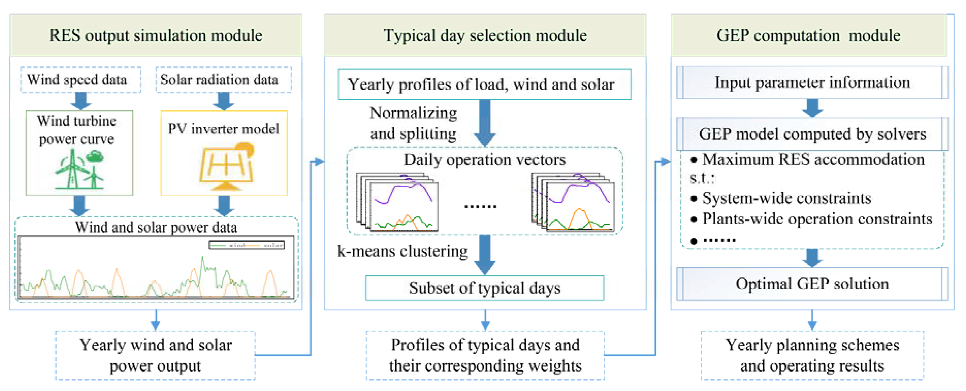
3. Solution Framework

The solution framework for solving the proposed GEP model is demonstrated systematically in Figure 1. Our solution framework contains three modules, i.e., RES output simulation module, typical day selection module, and GEP computation module. The first two modules provide input information for our proposed GEP model, and the final module is used to solve our proposed GEP model. Details of three modules in our solution framework are introduced as below.

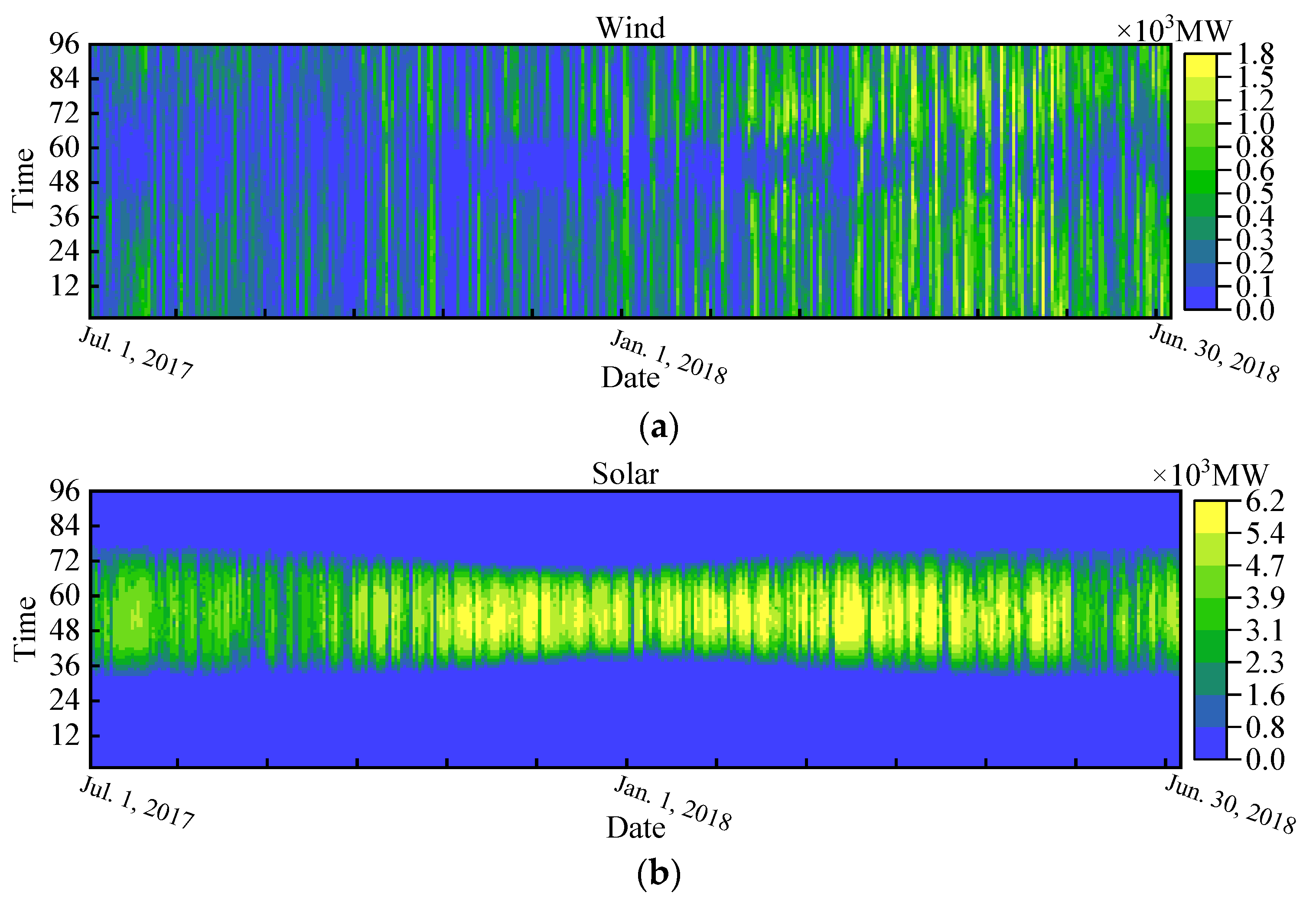
3.1. RES Output Simulation Module

The first module was used to simulate RES output at each wind or solar power plant, since no historical data of RES output are available for GEP problems [38]. In this module, we first assume that wind speed follows the Weibull distribution. Given the probability density mentioned above, the stochastic differential equation proposed by [39] is then used to generate time series of wind speed in all potential wind power plants. After that, hourly wind speed data are transferred into hourly wind power data through the typical wind turbine power curve. As for solar output simulation, we use the methodology proposed in [40] to first generate the daily clearness index. Then, an hourly solar radiation in PV panel is obtained by combining the daily clearness index and incoming solar radiation data. After that, hourly solar radiation data are transferred into hourly solar power data through the typical PV inverter model. Finally, wind and solar simulation data generated by this model are sent to the next module.

3.2. Typical Day Selection Module

Our proposed GEP model would become very computationally challenging if it contains operation constraints of all days in one year. To address this challenge, the second module was designed to select a subset of representative days and reduce the model complexity before solving our proposed GEP problems. Yearly profiles of load, wind, and solar are first normalized and then split into daily profiles of 365 days, respectively. Then, a high-dimensional vector (called “daily operating vector”) is constructed by putting a daily load profile, daily wind profile, and daily solar profile of the same day together [32]. Next, the well-known k-means clustering algorithm [41] is used to cluster all daily operating vectors, yielding a subset of representative days that capture a wide variety of operating conditions (including load, wind, and solar) in different seasons. The typical day selection process introduced above would be repeated to generate all representative days of every year over the planning horizon. Finally, load, wind, and solar profiles of representative days provide information for $D_{y,k,t}$, ${\varphi }_{i,y,k,t}^{\mathrm{W}}$, ${\varphi }_{i,y,k,t}^{\mathrm{S}}$ of our proposed GEP model, respectively. The weight of a representative day ${\omega }_{y,k}$ is calculated as the vector number in each cluster, divided by the total number of daily vectors.

3.3. GEP Computation Module

The previous two modules provide necessary parameter information, such as wind and solar profiles of representative days, for our proposed GEP model. In the final module, we used commercial solvers (for example, CPLEX) to efficiently solve our proposed GEP model, since this model is a MILP problem. After that, the GEP results and operating results of every year over the planning horizon were obtained. The RES accommodation results were calculated by scaling the obtained operating results via the weight of each representative day.

4. Results and Discussion

In this section, a testing system of one province in China is used to verify the effectiveness of our proposed GEP model. Numerical results from our proposed model and the traditional model are compared. All computations are carried out in C++ environment and MILP problems are solved by CPLEX on a desktop computer with 16 GB of RAM and a processor clocking at 3.40 GHz. When using CPLEX to solve MILP problems, the optimality gap is set to 0.01%.

4.1. Case Data

An actual power grid of one province located in Northwest China is modified as the testing system used in case studies, who has very rich resource of hydro energy and solar energy. In this system, its power generation mainly comes from hydro, thermal, wind and solar power plants. The installed capacity of all types of power generation in 2018 is summarized in

Table 1. The installed and potential capacity of different types of power generations in the testing system.

Type	Installed Capacity [GW] (2018)	Potential Capacity [GW] (2025)
Thermal	3.55	7.70
Hydro	10.86	16.92
Wind	2.05	5.55
Solar	9.42	18.92

. As indicated by Table 1, the installed capacity from wind and solar power plants has already reached 44% of the total capacity in 2018. On the other hand, the proportion of hydro power capacity is nearly 42%. Hence, almost all electricity demand in this testing system is provided by clean energy resources.

We choose historical data of the chosen area to simulate RES output for solving our proposed GEP model. Time-series data of wind and solar power outputs with 15-min time resolution from July 1, 2017 to June 30, 2018 (365 days in total) are visualized via the heat map in Figure 2. Note that Figure 2 shows the total power generated from all wind or solar plants in the testing system.

The planning horizon is set as from 2021 to 2025 and the discount rate r takes the value of 10%. The potential capacity of all types of power generation in 2025 is also shown in Table 1. The peak load of this system in 2018 is 9.25 GW and the annual growth rate of its peak load is expected to be 8% in future. The static reserve rate of each year $R_y^{\mathrm{D}}$ is set as 15% according to [42]. The transmission bias ${\delta }_l^{\mathrm{Tie}}$ is fixed as 5% in this paper. All capacity information mentioned above is available in [43,44,45].

All parameters of candidate units used in our case studies are shown in

Table 2. Parameters of candidate units for thermal power plant.

Plant	Maximum/ Minimum Capacity [MW]	Maximum Allowed Number	Capital Cost [k$/MW]	Fixed O&M Cost [k$/MW-yr]	Life [yr]	Ramping Up/Down Rate [MW/h]	Carbon Emission Rate [kg/MWh]	Minimum Up/Down Time [h]	Start-up/Shut-down Cost [$/MW]	Fuel Cost [$/MWh]
Coal1	138/82.8	4	571	11	40	41.4	852	4	99	18.3
Coal2	260/156	2	583	12	40	78	839	4	186	18.0
Coal3	330/198	2	589	12	40	132	831	8	236	17.8
Coal4	350/210	2	594	12	40	140	825	8	250	17.7
Coal5	660/330	2	500	10	40	198	817	8	471	17.5
Gas	200/40	2	494	10	40	200	424	2	143	57.3

,

Table 3. Parameters of candidate units for hydro power plant.

Plant	Maximum/ Minimum Capacity [MW]	Maximum Allowed Number	Capital Cost [k$/MW]	Fixed O&M Cost [k$/MW-yr]	Life [yr]	Ramping Up/Down Rate [MW/h]
Hydro1	120/0	6	1600	32	50	120
Hydro2	300/0	6	1607	32	50	300
Hydro3	320/0	6	1621	32	50	320
Hydro4	400/0	4	1629	32	50	400

,

Table 4. Parameters of candidate units for wind power plant.

Plant	Maximum/ Minimum Capacity [MW]	Maximum Allowed Number	Capital Cost [k$/MW]	Fixed O&M Cost [k$/MW-yr]	Life [yr]
Wind1	50/0	10	1071	43	35
Wind2	300/0	10	1071	43	35

and

Table 5. Parameters of candidate units for solar power plant.

Plant	Maximum/ Minimum Capacity [MW]	Maximum Allowed Number	Capital Cost [k$/MW]	Fixed O&M Cost [k$/MW-yr]	Life [yr]
Solar1	50/0	50	1029	41	30
Solar2	100/0	40	1029	41	30
Solar3	150/0	20	1029	41	30

. These parameters are public and come from [43,46]. The exchange rate between USD and RMB is set to 7 in this paper. On the other hand, it is assumed that all parameters will not change in the planning horizon. This means that we do not consider the influence of technology advances on all parameters of power plants. Since we do not consider the investment on the transmission system in this paper, the grid structure in the planning horizon is supposed to be the same with the structure of the year 2018.

4.2. Results

To verify the effectiveness of our proposed approach, we compare results of two GEP models. These two models are specified as follows.

• GEP-TO: This refers to the traditional GEP approach. Its objective is to find the least-cost generation mix. The total cost considered in GEP-TO model consists of the investment cost, the fixed operation and maintenance (O&M) costs, the fuel cost and the start-up cost of thermal plants.
• GEP-NO: This refers to our proposed GEP model with the alternative objective of maximizing the accommodation of RES. Our GEP-NO model is formulated by (1)–(24).

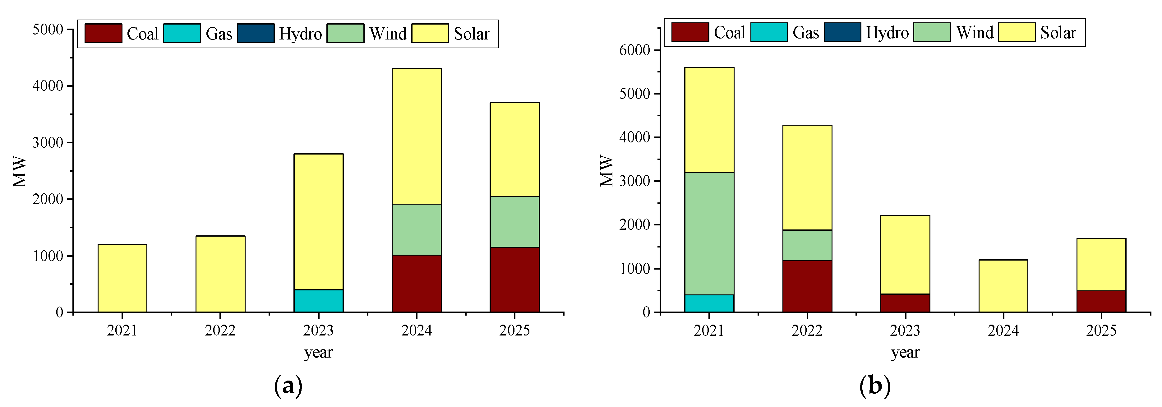
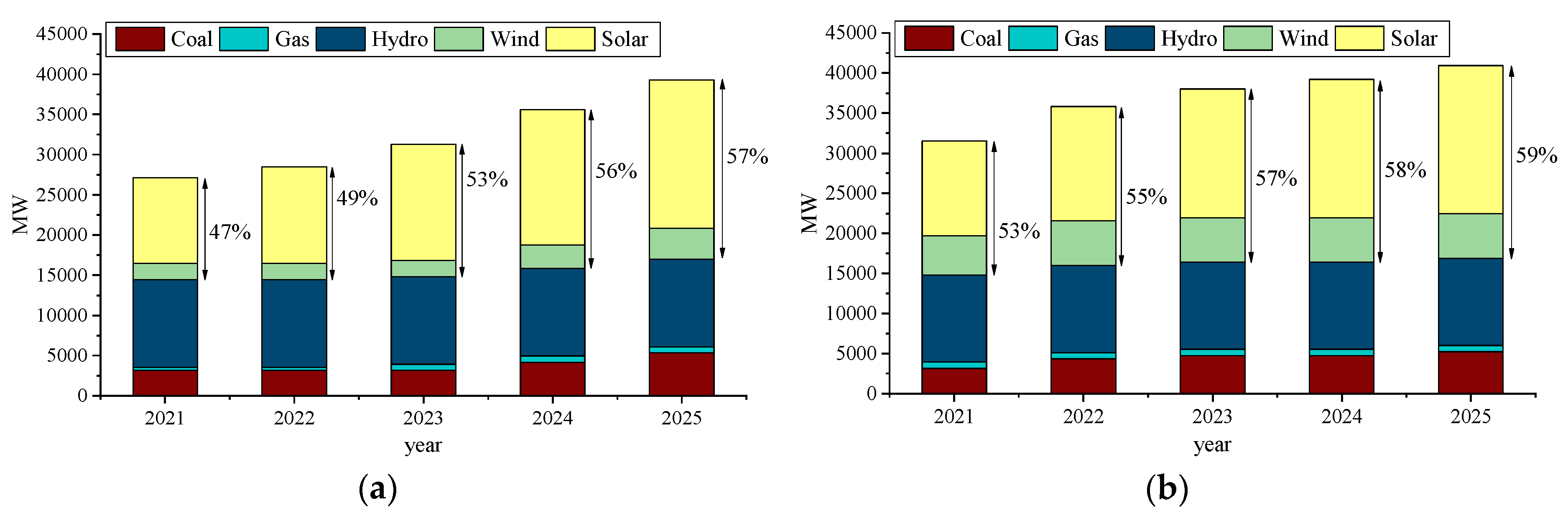
4.2.1. Comparison of the Installed Capacity between GEP-TO and GEP-NO

The installed capacity of each year obtained from GEP-TO and GEP-NO models is compared in Figure 3. Detailed planning results including yearly installed capacity and yearly investment cost of GEP-TO and GEP-NO models are given in

Table 6. Comparison of planning results between GEP-TO and GEP-NO models.

Year	Plant Type	GEP-TO		GEP-NO
		Installed Capacity (MW)	Investment Cost (Billion $)	Installed Capacity (MW)	Investment Cost (Billion $)
2021	Thermal	0	0.131	0	0.593
	Gas	0		400
	Wind	0		2800
	Solar	1200		2400
2022	Thermal	0	0.134	1180	0.373
	Gas	0		0
	Wind	0		700
	Solar	1350		2400
2023	Thermal	0	0.233	414	0.182
	Gas	400		0
	Wind	0		0
	Solar	2400		1800
2024	Thermal	1010	0.313	0	0.098
	Gas	0		0
	Wind	900		0
	Solar	2400		1200
2025	Thermal	1148	0.234	488	0.109
	Gas	0		0
	Wind	900		0
	Solar	1650		1200
Total		13,358	1.046	14,982	1.356

. From Figure 3a, we can observe that GEP-TO approaches install many solar power plants every year. This is mainly because GEP-TO model uses the least cost as its objective and solar power plants have lower investment cost than wind power plants. Another reason is that there are more solar resources in the testing system, as shown in Table 4 and Table 5. Wind power plants are installed until the year 2024. With the load growth every year, other two types of power generation are also installed in GEP-TO model. 400 MW of gas power units are added in 2023. Coal fired units are installed in 2024 and 2025.

In comparison with the traditional GEP-TO model, to increase the accommodation of RES generation, our proposed GEP-NO model installs 2800 MW of wind power capacity and 2400 MW of solar power capacity in the first year as shown in Figure 3b. However, GEP-TO model only installs 1200 MW of solar power capacity and no wind power capacity in the first year. In the second year, our proposed GEP-NO model installs 700 MW of wind power capacity and 2400 MW of solar power capacity, which are also significantly larger than 1350 MW of solar power capacity installed by the traditional GEP-TO model. Another difference is that thermal power plants (including coal fired and gas units) are installed in GEP-NO model every year except for the year of 2024. But, the installed capacity of thermal power plant every year is relatively small in GEP-NO model. Because of the high investment cost, no hydro power plants are installed during the planning horizon in both GEP-NO and GEP-TO models.

From Figure 3 and Table 6, it can be seen that GEP-NO model prefers to install both renewable power plants and thermal power plants simultaneously. And, more renewable power plants would be installed in our proposed GEP-NO model compared with the traditional GEP-TO model. On the other hand, these renewable power plants are also installed much earlier in our proposed GEP-NO model than the traditional GEP-TO model. Thus, more RES generation could be accommodated in GEP-NO model, although the total investment of GEP-NO model is a little bit higher than that of GEP-TO model.

4.2.2. Comparison of the Generation Mix between GEP-TO and GEP-NO

Figure 4 presents the generation mix of GEP-TO and GEP-NO models every year over the planning horizon. Detailed yearly cumulative installed capacity of all plant types and total installed capacity results of the two models are provided in

Table 7. Comparison of cumulative installed capacity of all plant types and total installed capacity results between GEP-TO and GEP-NO models.

Year	Plant Type	GEP-TO		GEP-NO
		Cumulative Installed Capacity (MW)	Total Installed Capacity (MW)	Cumulative Installed Capacity (MW)	Total Installed Capacity (MW)
2021	Thermal	3160	27,126	3160	31,526
	Gas	390		790
	Hydro	10,875		10,875
	Wind	2045		4845
	Solar	10,656		11,856
2022	Thermal	3160	28,476	4340	35,806
	Gas	390		790
	Hydro	10,875		10,875
	Wind	2045		5545
	Solar	12,006		14,256
2023	Thermal	3160	31,276	4754	38,020
	Gas	790		790
	Hydro	10,875		10,875
	Wind	2045		5545
	Solar	14,406		16,056
2024	Thermal	4170	35,586	4754	39,220
	Gas	790		790
	Hydro	10,875		10,875
	Wind	2945		5545
	Solar	16,806		17,256
2025	Thermal	5318	39,284	5242	40,908
	Gas	790		790
	Hydro	10,875		10,875
	Wind	3845		5545
	Solar	18,456		18,456

. As indicated in Figure 4, compared with the proportion (44%) of wind & solar energy in 2018, both GEP-TO and GEP-NO models increase the share of wind and solar energy year after year from 2021 to 2025. However, our proposed GEP-NO model increases the proportion of wind & solar energy more rapidly than the traditional GEP-TO model. Specifically, in the first year (2021), the share of wind & solar energy in GEP-NO model has already reached 53%, which is significantly larger than that in GEP-TO model (only 47%). In the last year (2025), GEP-NO model yields to 59% of wind and solar energy, which is also larger than 57% in GEP-TO model. Reasons for a higher share of RES generation in GEP-NO model than GEP-TO model are that more wind power capacity are installed in our proposed GEP-NO model in the first year (2021). This also increases the accommodation of RES generation over the planning horizon. As demonstrated in Table 7, the cumulative installed capacity of all plant types except hydro plant type has been increased at various levels since the first year of the planning horizon in the two models. Specifically, solar resource in both GEP-TO and GEP-NO models has nearly reached its potential capacity in the last year (the cumulative installed capacity of solar plants in both models is 18456 MW), while in GEP-NO model there is no potential capacity left for wind resource (5545 MW). The total capacity of GEP-NO model in the last year is 40908 MW, which is 1624 MW larger than that of GEP-TO model. Accordingly, the extra installed capacity results in the additional investment cost in GEP-NO model.

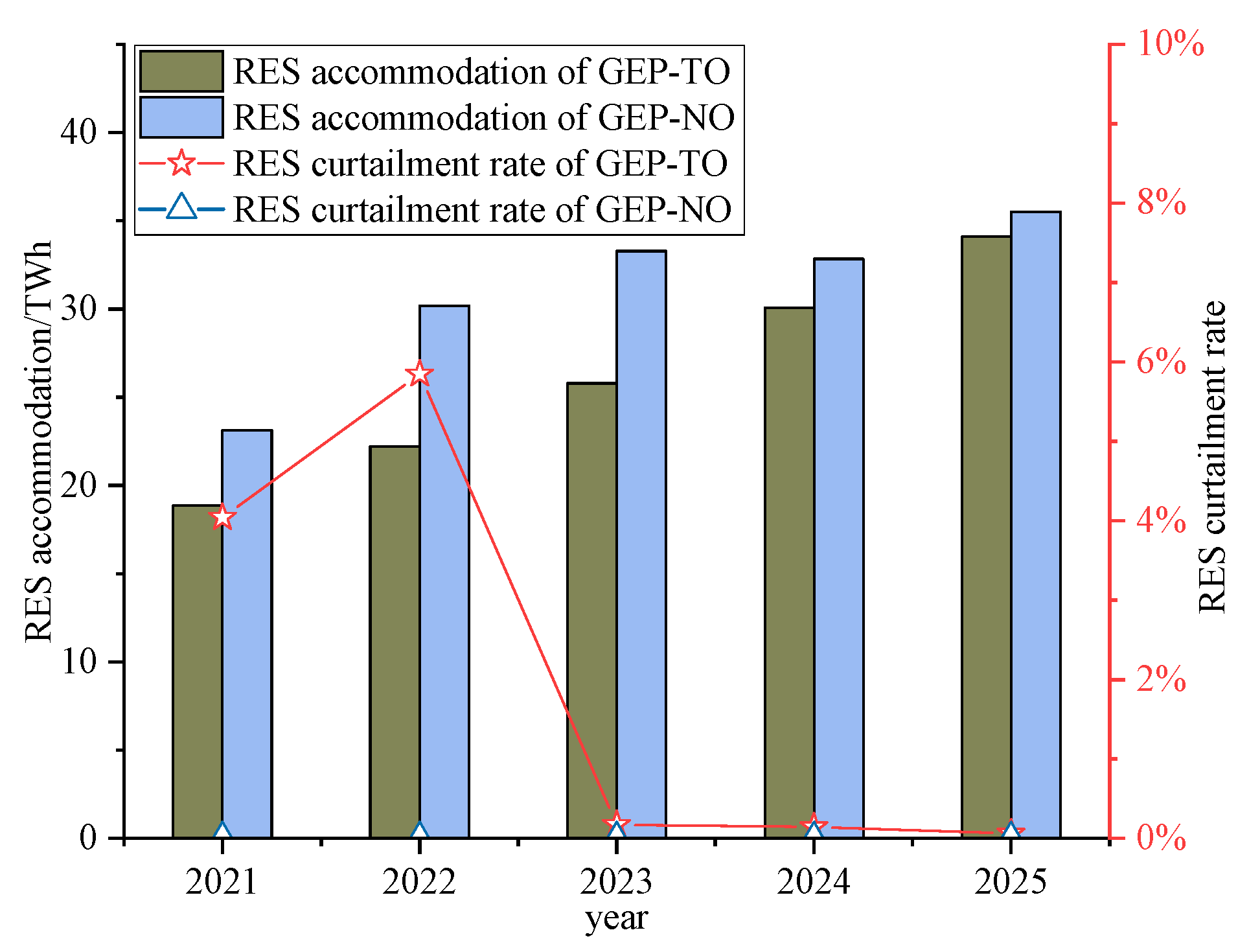
4.2.3. Comparison of the RES Accommodation and Curtailment between GEP-TO and GEP-NO

RES accommodation and curtailment of GEP-TO and GEP-NO models are shown and compared in Figure 5 and

Table 8. Comparison of the amount of RES accommodation and curtailment between GEP-TO and GEP-NO models.

Year	RES Accommodation (TWh)		RES Curtailment (TWh)
	GEP-TO	GEP-NO	GEP-TO	GEP-NO
2021	18.873	23.126	0.794	0.000
2022	22.208	30.183	1.379	0.000
2023	25.794	33.282	0.045	0.000
2024	30.061	32.840	0.044	0.000
2025	34.092	35.498	0.021	0.000

. In this paper, only wind and solar energy are considered as RES. From Figure 5 and Table 8, it can be seen that RES accommodation in GEP-NO model is higher than that in GEP-TO model every year. The five-year electricity generated from RES in GEP-NO model is 154.93 TWh, much larger than 131.03 TWh in GEP-TO model. No RES is curtailed in GEP-NO model. However, RES curtailment has occurred in GEP-TO model over the five-year period, with the maximum curtailment amount of 1.379 TWh and the curtailment rate of 5.85% in the year of 2022. These show that our proposed GEP-NO model can significantly improve RES accommodation and reduce RES curtailment compared to the traditional GEP-TO model.

On the other hand, GEP-NO model accommodates more RES generation in the first three years (from 2021 to 2023) than GEP-TO model. Specially, in 2022 and 2023, compared with GEP-TO model, our proposed GEP-NO model increases the RES accommodation by 7.98 TWh and 7.49 TWh, respectively. This is because more wind and solar generation are installed in the first three years, as demonstrated in Table 6. However, in the last two years, the difference of RES accommodation between GEP-TO and GEP-NO models is relatively small, only 2.78 TWh in 2024 and 1.41 TWh in 2025. This is because almost all of wind and solar resource have been developed and there is no enough potential RES available for GEP in the last two years. As presented in Table 8, a considerable amount of renewable energy in GEP-TO model is curtailed in the first two years, to be precise, 0.794 TWh in 2021 and 1.379 TWh in 2022. In the following three years, the amount of yearly RES curtailment of GEP-TO model falls to less than 0.05 TWh. By contrast, no RES curtailment has occurred in GEP-NO model over the five years. One reason is that some dispatchable units like gas power units and coal fired units are installed in first two years in GEP-NO model compared with GEP-TO model, as illustrated in Figure 3. It should be clarified that the amount of RES accommodation and curtailment in both models are computed without considering the transmission network of the chosen region. A multi-period GEP model with a network-constrained unit commitment model will be studied in further research.

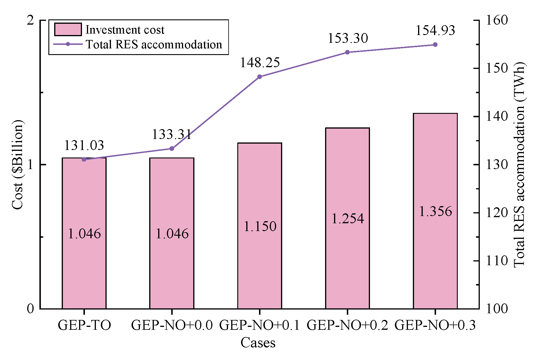
4.2.4. Sensitive Analysis of Key Control Parameters

The investment cost budget is a critical parameter in our proposed GEP model. In other words, decision makers would set up the desired budget level according to their trade-off between the economy and RES accommodation. Planning results may change greatly at distinct levels of investment cost budget, which generally yields to different RES accommodation results. To analyze the impact of investment cost budget on planning schemes and RES accommodation, we choose the investment cost obtained by GEP-TO model as the benchmark, and then four subcases with different investment rates are designed based on GEP-NO model, defined as follows:

• GEP-NO+0.0: The rate of the investment cost of GEP-NO model is 1 time (1+0.0) that of GEP-TO model.
• GEP-NO+0.1: The rate of the investment cost of GEP-NO model is 1.1 times (1+0.1) that of GEP-TO model.
• GEP-NO+0.2: The rate of the investment cost of GEP-NO model is 1.2 times (1+0.2) that of GEP-TO model.
• GEP-NO+0.3: The rate of the investment cost of GEP-NO model is 1.3 times (1+0.3) that of GEP-TO model.

Figure 6 shows the comparison of investment cost and total RES accommodation between GEP-TO and GEP-NO models with different investment rates. As indicated in Figure 6, with the growing rate, the total RES accommodation in all four subcases of GEP-NO model increases accordingly, from 133.31 to 154.93 TWh. Compared with GEP-TO model, GEP-NO+0.0 model increases RES accommodation by 2.28 TWh although their investment costs are the same. By contrast, the accommodation of RES in GEP-NO+0.1 model is 14.94 TWh higher than that in GEP-NO+0.0 model because more wind and solar power plants are installed in the first two years. The difference of RES accommodation between GEP-NO+0.1 and GEP-NO+0.2 model is 5.05 TWh. However, the growth of RES accommodation slows down (only 1.63 TWh) when the investment cost rate rises from 1.2 to 1.3, since the additional investment cost brings only a small number of installed renewable units and they are mainly installed in the end of the planning period.

4.2.5. Proposals of management implications

Though the deployment of RES has been increased strongly in the past decade, how to invest RES reasonably to meet the goal of sustainable development and ensure RES accommodation as much as possible is still challenging for decision makers in power systems. Based on planning results in our case studies, some management implications are proposed as suggestions for decision makers:

• For some cost-oriented cases, the traditional GEP model would yield to a least-cost planning scheme, while it could not guarantee renewable energy generation to be fully utilized.
• The proposed GEP model with the objective of maximizing RES accommodation could be applied in the case with very rich renewable energy resource. Although our proposed model may result in more investment cost, it can increase the accommodation of RES efficiently and reduce the amount of RES curtailment.
• The selection of the investment cost budget (presented in constraint (2)) in our proposed GEP model depends on the conservative level of decision makers. Compared to a risk-averser, a risk-taker would be willing to pay more to install more RES and accommodate more renewable energy. Therefore, the investment cost would be higher. On the other hand, the investment cost budget in our proposed model can be determined by a two-stage method. In the first stage, the traditional GEP model is calculated to obtain the optimal investment cost over the planning period. Then in the second stage, decision makers can set up their desired investment budget, which is somewhat higher than the optimal investment cost derived from the first stage. After that, our proposed GEP model can be computed with this investment budget.

5. Conclusions

In this paper, we proposed a novel generation expansion planning (GEP) approach for power systems with high penetration of renewable energy. This model contains short-term operating constraints and an alternative objective to maximize the accommodation of renewable energy sources (RES). To make our proposed GEP model computational tractable, k-means clustering is used to select a subset of representative days and reduce the model complexity.

The effectiveness of our proposed model is verified on a real system in one province of China with high penetration of RES. Numerical results indicate that our proposed GEP model prefers to install more renewable power plants much earlier than the traditional GEP model with the objective to minimize the total investment cost. Although its total investment cost is a little bit higher than the traditional model, more RES generation could be accommodated in our proposed GEP model. Thus, our proposed approach provides better planning results to increase the utilization of renewable energy and reduce the renewable energy curtailment. Meanwhile, decision makers in power systems should make the tradeoff between the total cost and the accommodation of RES. More accommodation of RES is generally realized by allowing more investment in renewable energy generation.

References

1. Sadeghi, H.; Rashidinejad, M.; Abdollahi, A. A comprehensive sequential review study through the generation expansion planning. Renew. Sustain. Energy Rev. 2017, 67, 1672–1682. [Google Scholar] [CrossRef]
2. Koltsaklis, N.E.; Dagoumas, A.S. State-of-the-art generation expansion planning: A review. Appl. Energy 2018, 230, 563–589. [Google Scholar] [CrossRef]
3. Conejo, A.J.; Baringo, L.; Jalal Kazempour, S.; Siddiqui, A.S. Investment in Electricity Generation and Transmission: Decision Making under Uncertainty; Springer International Publishing: Cham, Switzerland, 2016; ISBN 9783319295015. [Google Scholar]
4. Roh, J.H.; Shahidehpour, M.; Fu, Y. Market-based coordination of transmission and generation capacity planning. IEEE Trans. Power Syst. 2007, 22, 1406–1419. [Google Scholar] [CrossRef]
5. Khodaei, A.; Shahidehpour, M.; Wu, L.; Li, Z. Coordination of short-term operation constraints in multi-area expansion planning. IEEE Trans. Power Syst. 2012, 27, 2242–2250. [Google Scholar] [CrossRef]
6. Wang, P.; Wang, C.; Hu, Y.; Varga, L.; Wang, W. Power generation expansion optimization model considering multi-scenario electricity demand constraints: A case study of Zhejiang province, China. Energies 2018, 11, 1498. [Google Scholar] [CrossRef] [Green Version]
7. Alizadeh, B.; Jadid, S. A dynamic model for coordination of generation and transmission expansion planning in power systems. Int. J. Electr. Power Energy Syst. 2015, 65, 408–418. [Google Scholar] [CrossRef]
8. Munoz, F.D.; Watson, J.P. A scalable solution framework for stochastic transmission and generation planning problems. Comput. Manag. Sci. 2015, 12, 491–518. [Google Scholar] [CrossRef]
9. Wang, X.; McDonald, J.R. Modern Power System Planning; McGraw-Hill Companies: New York, NY, USA, 1994. [Google Scholar]
10. Brouwer, A.S.; van den Broek, M.; Seebregts, A.; Faaij, A. Operational flexibility and economics of power plants in future low-carbon power systems. Appl. Energy 2015, 156, 107–128. [Google Scholar] [CrossRef] [Green Version]
11. Chen, Q.; Kang, C.; Xia, Q.; Zhong, J. Power generation expansion planning model towards low-carbon economy and its application in China. IEEE Trans. Power Syst. 2010, 25, 1117–1125. [Google Scholar] [CrossRef] [Green Version]
12. Billinton, R.; Gao, Y.; Karki, R. Application of a joint deterministic-probabilistic criterion to wind integrated bulk power system planning. IEEE Trans. Power Syst. 2010, 25, 1384–1392. [Google Scholar] [CrossRef]
13. Connolly, D.; Lund, H.; Mathiesen, B.V.; Leahy, M. A review of computer tools for analysing the integration of renewable energy into various energy systems. Appl. Energy 2010, 87, 1059–1082. [Google Scholar] [CrossRef]
14. Kim, J.; Kim, K. Integrated model of economic generation system expansion plan for the stable operation of a power plant and the response of future electricity power demand. Sustainability 2018, 10, 2417. [Google Scholar] [CrossRef] [Green Version]
15. Poncelet, K.; Delarue, E.; Six, D.; Duerinck, J.; D’haeseleer, W. Impact of the level of temporal and operational detail in energy-system planning models. Appl. Energy 2016, 162, 631–643. [Google Scholar] [CrossRef] [Green Version]
16. Gacitua, L.; Gallegos, P.; Henriquez-Auba, R.; Lorca, Á.; Negrete-Pincetic, M.; Olivares, D.; Valenzuela, A.; Wenzel, G. A comprehensive review on expansion planning: Models and tools for energy policy analysis. Renew. Sustain. Energy Rev. 2018, 98, 346–360. [Google Scholar] [CrossRef]
17. Turvey, R.; Anderson, D. Electricity Economics: Essays and Case Studies; World Bank by Johns Hopkins University Press: Baltimore, MD, USA, 1977. [Google Scholar]
18. Baringo, L.; Conejo, A.J. Correlated wind-power production and electric load scenarios for investment decisions. Appl. Energy 2013, 101, 475–482. [Google Scholar] [CrossRef]
19. Ding, T.; Hu, Y.; Bie, Z. Multi-stage stochastic programming with nonanticipativity constraints for expansion of combined power and natural gas systems. IEEE Trans. Power Syst. 2017, 33, 317–328. [Google Scholar] [CrossRef]
20. Kazempour, S.J.; Conejo, A.J.; Ruiz, C. Strategic generation investment using a complementarity approach. IEEE Trans. Power Syst. 2011, 26, 940–948. [Google Scholar] [CrossRef]
21. Zhang, Y.; Wang, J.; Zeng, B.; Hu, Z. Chance-constrained two-stage unit commitment under uncertain load and wind power output using bilinear benders decomposition. IEEE Trans. Power Syst. 2017, 32, 3637–3647. [Google Scholar] [CrossRef] [Green Version]
22. Koltsaklis, N.E.; Georgiadis, M.C. A multi-period, multi-regional generation expansion planning model incorporating unit commitment constraints. Appl. Energy 2015, 158, 310–331. [Google Scholar] [CrossRef]
23. Lu, Z.; Li, H.; Qiao, Y. Probabilistic flexibility evaluation for power system planning considering its association with renewable power curtailment. IEEE Trans. Power Syst. 2018, 33, 3285–3295. [Google Scholar] [CrossRef]
24. Khastieva, D.; Dimoulkas, I.; Amelin, M. Optimal investment planning of bulk energy storage systems. Sustainability 2018, 10, 610. [Google Scholar] [CrossRef] [Green Version]
25. Shortt, A.; Kiviluoma, J.; O’Malley, M. Accommodating variability in generation planning. IEEE Trans. Power Syst. 2013, 28, 158–169. [Google Scholar] [CrossRef]
26. Wogrin, S.; Duenas, P.; Delgadillo, A.; Reneses, J. A new approach to model load levels in electric power systems with high renewable penetration. IEEE Trans. Power Syst. 2014, 29, 2210–2218. [Google Scholar] [CrossRef]
27. Han, X.; Liao, S.; Ai, X.; Yao, W.; Wen, J. Determining the minimal power capacity of energy storage to accommodate renewable generation. Energies 2017, 10, 468. [Google Scholar] [CrossRef] [Green Version]
28. Palmintier, B.S.; Webster, M.D. Impact of operational flexibility on electricity generation planning with renewable and carbon targets. IEEE Trans. Sustain. Energy 2016, 7, 672–684. [Google Scholar] [CrossRef]
29. Abdin, I.F.; Zio, E. An integrated framework for operational flexibility assessment in multi-period power system planning with renewable energy production. Appl. Energy 2018, 222, 898–914. [Google Scholar] [CrossRef] [Green Version]
30. Chen, X.; Lv, J.; McElroy, M.B.; Han, X.; Nielsen, C.P.; Wen, J. Power system capacity expansion under higher penetration of renewables considering flexibility constraints and low carbon policies. IEEE Trans. Power Syst. 2018, 33, 6240–6253. [Google Scholar] [CrossRef]
31. Du, E.; Zhang, N.; Kang, C.; Xia, Q. A high-efficiency network-constrained clustered unit commitment model for power system planning studies. IEEE Trans. Power Syst. 2018, 34, 2498–2508. [Google Scholar] [CrossRef]
32. Liu, Y.; Sioshansi, R.; Conejo, A.J. Hierarchical clustering to find representative operating periods for capacity-expansion modeling. IEEE Trans. Power Syst. 2018, 33, 3029–3039. [Google Scholar] [CrossRef]
33. Luo, G.L.; Li, Y.L.; Tang, W.J.; Wei, X. Wind curtailment of China’s wind power operation: Evolution, causes and solutions. Renew. Sustain. Energy Rev. 2016, 53, 1190–1201. [Google Scholar] [CrossRef]
34. Nikoobakht, A.; Aghaei, J.; Shafie-Khah, M.; Catalao, J.P.S. Assessing increased flexibility of energy storage and demand response to accommodate a high penetration of renewable energy sources. IEEE Trans. Sustain. Energy 2019, 10, 659–669. [Google Scholar] [CrossRef]
35. Wei, J.; Zhang, Y.; Wang, J.; Cao, X.; Khan, M.A. Multi-period planning of multi-energy microgrid with multi-type uncertainties using chance constrained information gap decision method. Appl. Energy 2020, 260, 114188. [Google Scholar] [CrossRef]
36. Ueckerdt, F.; Brecha, R.; Luderer, G. Analyzing major challenges of wind and solar variability in power systems. Renew. Energy 2015, 81, 1–10. [Google Scholar] [CrossRef]
37. Huang, H.; Liang, D.; Liang, L.; Tong, Z. Research on China’s power sustainable transition under progressively levelized power generation cost based on a dynamic integrated generation–transmission planning model. Sustainability 2019, 11, 2288. [Google Scholar] [CrossRef] [Green Version]
38. Zhang, Y.; Wang, J. K-nearest neighbors and a kernel density estimator for GEFCom2014 probabilistic wind power forecasting. Int. J. Forecast. 2016, 32, 1074–1080. [Google Scholar] [CrossRef]
39. Zhang, N.; Kang, C.; Duan, C.; Tang, X.; Huang, J.; Lu, Z.; Wang, W.; Qi, J. Simulation methodology of multiple wind farms operation considering wind speed correlation. Int. J. Power Energy Syst. 2010, 30, 264. [Google Scholar] [CrossRef]
40. Santos, J.M.; Pinazo, J.M.; Canada, J. Methodology for generating daily clearness index index values Kt starting from the monthly average daily value Kt. Determining the daily sequence using stochastic models. Renew. Energy 2003, 28, 1523–1544. [Google Scholar] [CrossRef]
41. Kotzur, L.; Markewitz, P.; Robinius, M.; Stolten, D. Impact of different time series aggregation methods on optimal energy system design. Renew. Energy 2018, 117, 474–487. [Google Scholar] [CrossRef] [Green Version]
42. Notice on the Issuance of the Risk Warning for Coal-Fired Power Planning and Construction in 2022. Available online: http://zfxxgk.nea.gov.cn/auto84/201904/t20190419_3655.htm (accessed on 27 March 2019).
43. Annual Report on the Development of China’s Power Industry in 2018. Available online: http://www.cec.org.cn/d/file/yaowenkuaidi/2018-06-14/a041f73a9cd2115d94e55d815f9b4b4e.pdf (accessed on 14 June 2018).
44. Wind Power Grid Connection and Operation in 2018. Available online: http://www.nea.gov.cn/2019-01/28/c_137780779.htm (accessed on 28 January 2019).
45. Photovoltaic Power Generation Statistics in 2018. Available online: http://www.nea.gov.cn/2019-03/19/c_137907428.htm (accessed on 19 March 2019).
46. Research on the Mechanism Reform of On-Grid Tariffs for China. Available online: http://www.raponline.org/wpcontent/uploads/2016/05/generationdispatchcompensationreform-cn-2016-mar.pdf (accessed on 24 March 2016).
Figure 1. Solution framework of the proposed generation expansion planning (GEP) model.
Sustainability 12 01083 g001
Figure 2. Wind and solar power outputs with 15-min time resolution from 1 July 2017 to 30 June 2018 in the testing system. (a): Total power outputs generated from all wind farms; (b): Total power outputs generated from all solar stations.
Sustainability 12 01083 g002
Figure 3. Comparison of the installed capacity between GEP-TO and GEP-NO models: (a) Installed capacity results of GEP-TO model; (b) Installed capacity results of GEP-NO model.
Sustainability 12 01083 g003
Figure 4. Comparison of the generation mix between GEP-TO and GEP-NO models (the percentage indicates the share of wind and solar power generation every year): (a) Generation mix results of GEP-TO model; (b) Generation mix results of GEP-NO model.
Sustainability 12 01083 g004
Figure 5. Comparison of RES accommodation and curtailment rate between GEP-TO and GEP-NO models.
Sustainability 12 01083 g005
Figure 6. Comparison of the investment cost and the total RES accommodation between GEP-TO and GEP-NO models with different investment cost rates.
Sustainability 12 01083 g006