A Neural Network-Based Sustainable Data Dissemination through Public Transportation for Smart Cities

Abstract

In recent years, there has been a big data revolution in smart cities dues to multiple disciplines such as smart healthcare, smart transportation, and smart community. However, most services in these areas of smart cities have become data-driven, thus generating big data that require sharing, storing, processing, and analysis, which ultimately consumes massive amounts of energy. The accumulation process of these data from different areas of a smart city is a challenging issue. Therefore, researchers have started aiming at the Internet of vehicles (IoV), in which smart vehicles are equipped with computing and storage capabilities to communicate with surrounding infrastructure. In this paper, we propose a subcategory of IoV as the Internet of buses (IoB), where public buses enable a service as a data carrier in a smart city by introducing a neural network-based sustainable data dissemination system (NESUDA), where opportunistic sensing comprises delay-tolerant data collection, processing and disseminating from one place to another place around the city. The objective was to use public transport to carry data from one place to another and to reduce the traffic from traditional networks and energy consumption. An advanced neural network (NN) algorithm was applied to locate the realistic arrival time of public buses for data allocation. We used the Auckland transport (AT) buses data set from the transport agency to validate our model for the level of accuracy in predicted bus arrival time and scheduled arrival time to disseminate data using bus services. Data were uploaded onto buses as per their dwelling time at each stop and terminals within the coverage area of deployed RSU. The offloading capacity of our proposed data dissemination system showed that it could be utilized to effectively complement traditional data networks. Moreover, the maximum offloading capacity at each parent stop could reach up to 360 GB with a huge saving of energy consumption.

1. Introduction

Nowadays, a huge surge in Internet traffic raises many concerns over the capacity of the infrastructure. All the mobile devices are equipped with wireless network interfaces and which introduce new demands in the wireless network leading to the digital society with the emerging trend of “big data” with features of high-volume, high-velocity, and high-variety. With a limited spectrum of resources, mobile operators may be struggling to provide adequate bandwidth to handle the amount of traffic generated by their users. These big data sources in a smart city are posing sustainability challenges to achieve ecosystem balance and, at the same time, perform the day-to-day data transmission activities. Therefore, recently, much attention has been focused on accommodating big data needs by leveraging the traffic burden from the traditional network to other networks, which is also known as data offloading. This technique helps to reduce the congestion over the conventional network and make bandwidth available for other users for effective usage. The Cisco visual networking index (VNI) [1] has revealed that fixed networks have been used to offload data from mobile data in 2019, and it was approximately 51% of total global traffic. Therefore, it is possible to offload data from the network to another available network as per the user’s preferences. Similarly, we also require an alternative approach to alleviate this pressure on the existing infrastructure. Thus, efficient data dissemination mechanisms considering the urban Internet bandwidth consumption should be designed. We consider in addition to the traditional network to shift traffic and improve bandwidth utilization. Therefore, Wi-Fi enabled and on-board unit (OBU) equipped buses and bus stops show the potential for forming the communication backbone. The main aim is to utilize public transport buses to carry data from one place to another place on their predefined route. Our public transport system exploits nearby communications, short-term storage at bus stops, and predictable bus movement to deliver non-real-time information. We used the public transport network due to their scheduled movement and fixed timetable. However, we noticed a delay in bus arrival time in real-life due to some uncertainties. Therefore, we applied an ANN algorithm to have more realistic information on bus arrival time at each bus stop. To validate our idea, we used Auckland Transport (AT) historical data to analyze bus daily movement patterns and applied an advanced neural network algorithm to understand the variance between predicted arrival time and schedule travel time for more realistic information to authenticate that public transport can be used as an energy-efficient communication channel. All public vehicles stop at bus stops for a long or short duration known as bus dwell time during their fixed travel route, and data were uploaded and downloaded at these bus stops only. It was important to be within the range of the interfaces for better and fast communication between bus stops and buses. We utilized the bus arrival time, departure time, and speed of all public buses to load and offload the data. However, there were some factors such as signals, traffic fluctuations, peak hours, and road incidents, which often lead to delay in set schedules and results in irregularities in journey times and bus arrival times. Many other factors are available that lead to the variation of public bus travel times, and some of these factors were not measurable. Unexpected delays could be predicted. However, we emphasize more on historical data provided by the transport agency and carry out analysis to get the most accurate prediction results. The main contributions of this paper are the following:

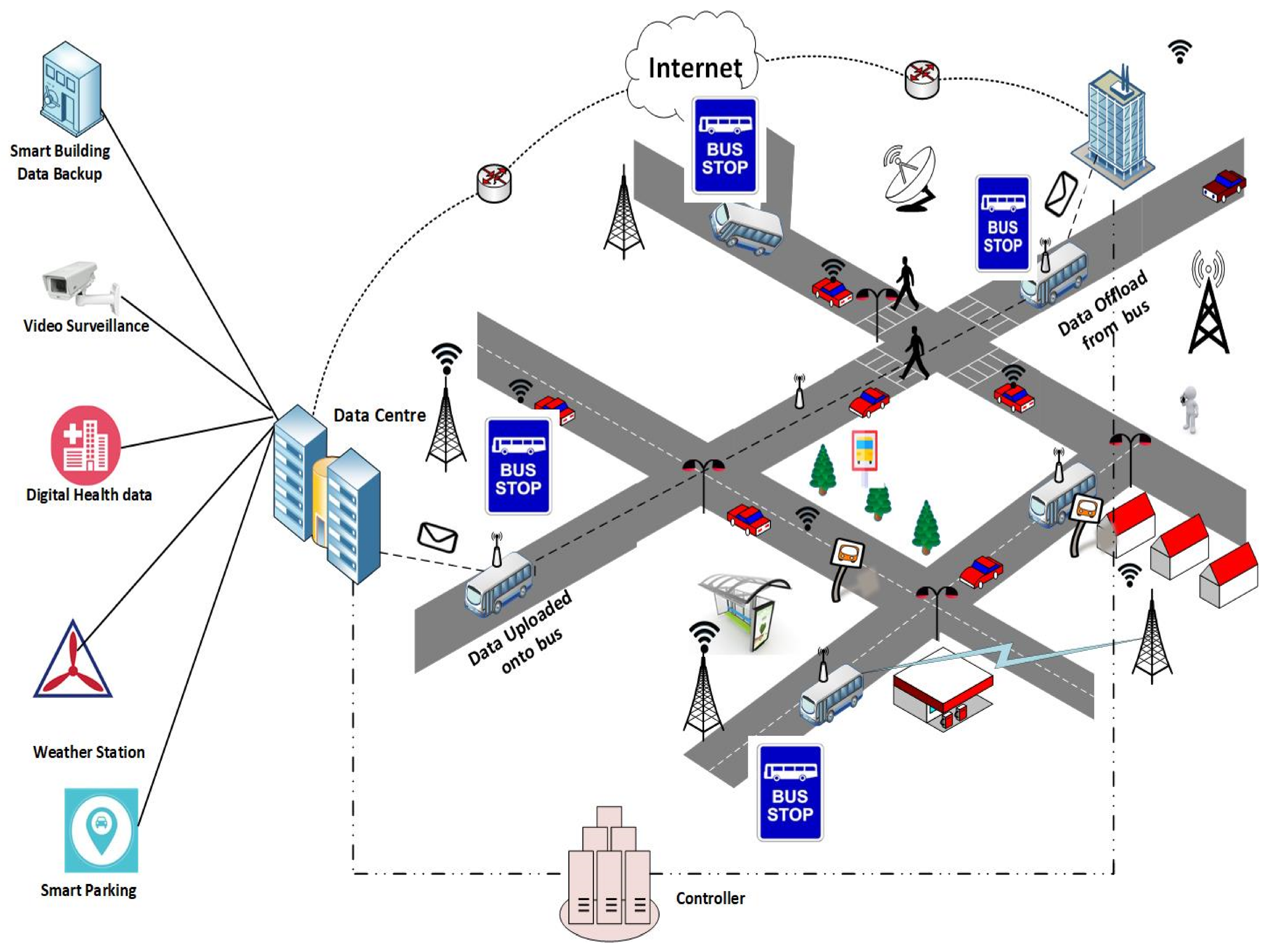
• We obtained the characterizations of the public transport bus systems that currently exist and determined bus daily movement patterns to form a data transmission network named as neural network-based sustainable data dissemination system (NESUDA).
• We applied the advanced neural network algorithm to analyze the arrival time based on historical data. We analyzed the difference between scheduled and predicted arrival times to estimate the accuracy of utilizing public buses for data dissemination. The Auckland transport data set was used to validate our model.
• We proposed a data dissemination algorithm using data scheduling onto buses as per their dwell time at each passing stop and stopping stop.
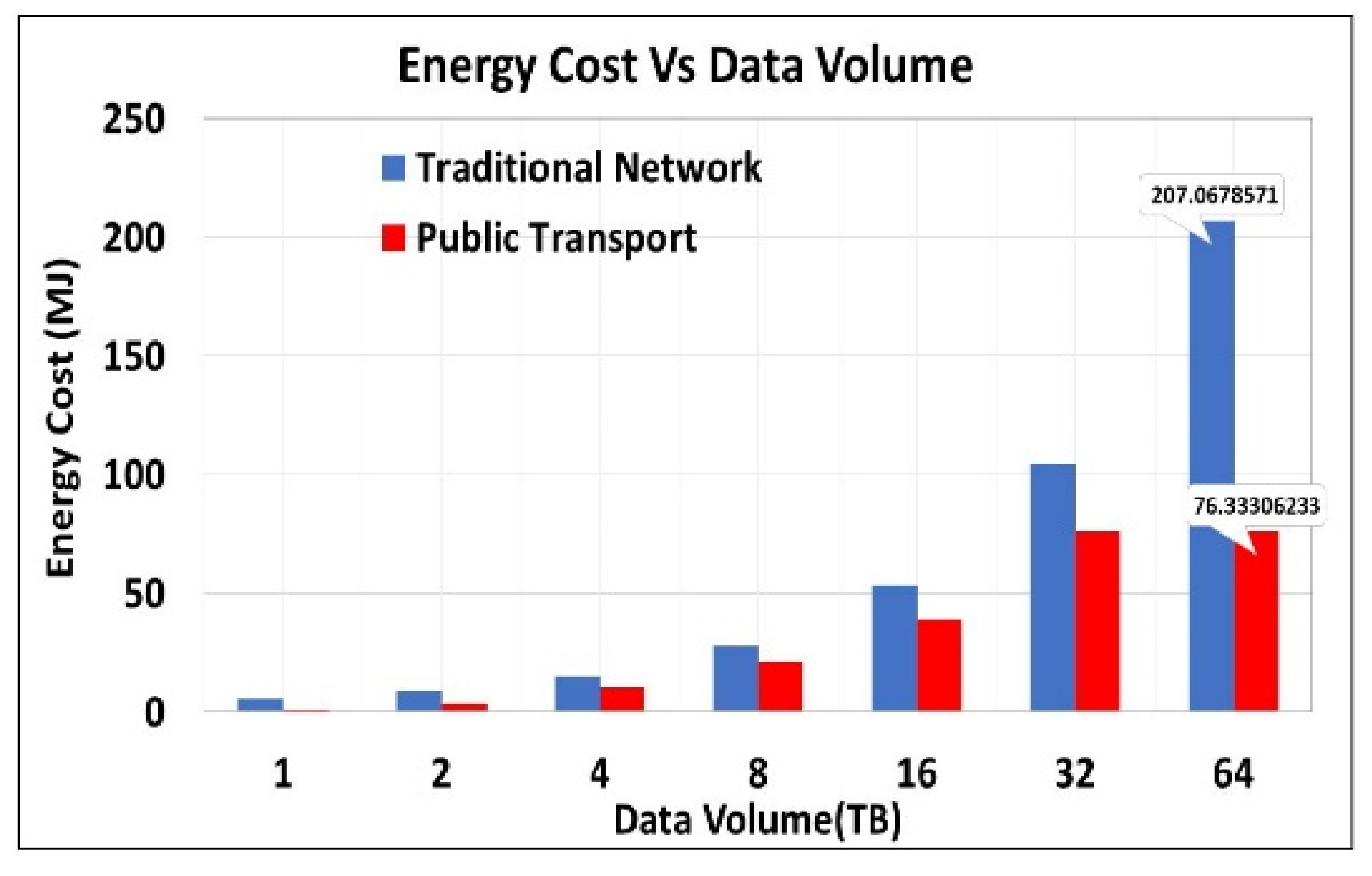
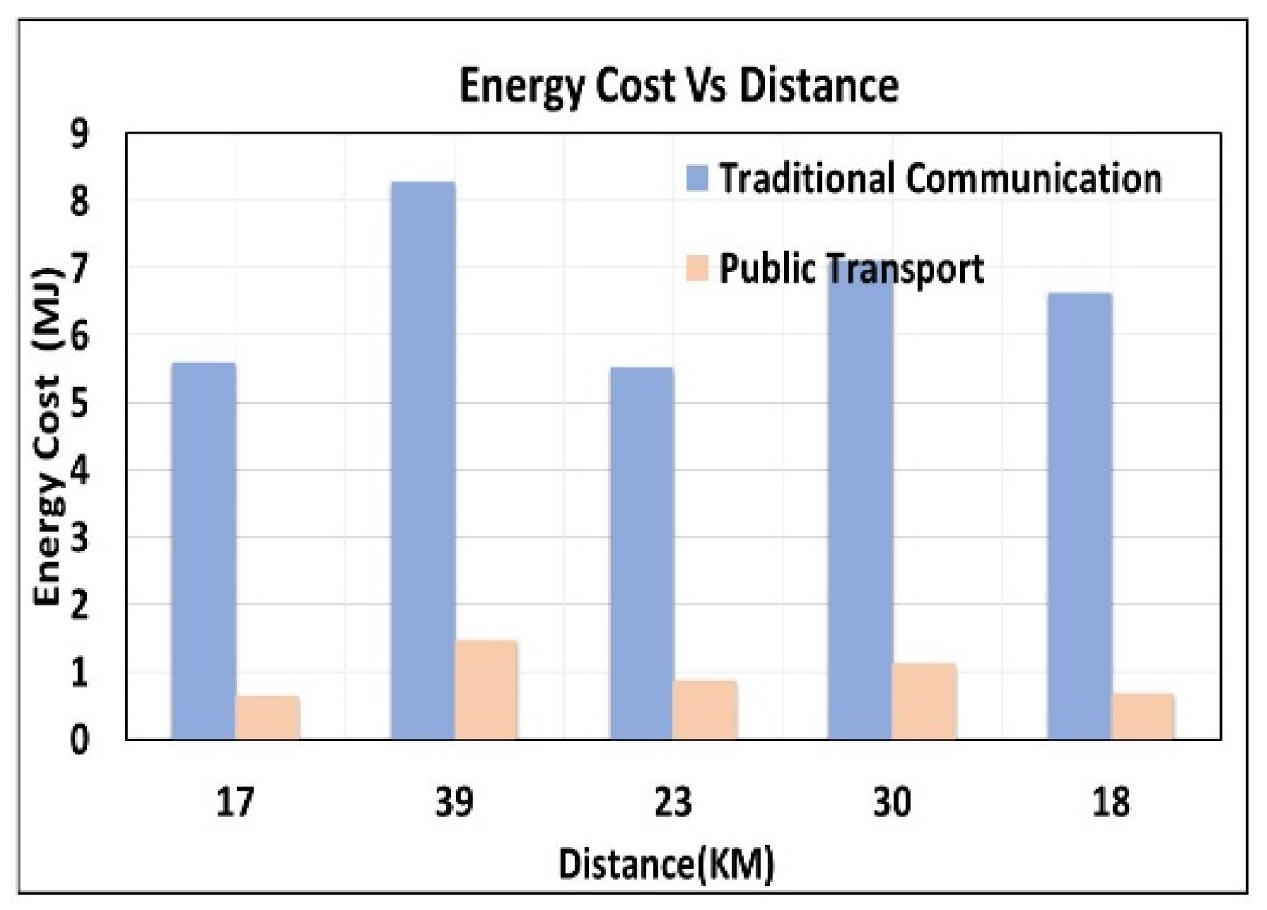
• For evaluation, a detailed comparative analysis of energy consumption is performed for traditional and vehicular networks.

The remainder of the paper is structured as follows: in Section 2, we present the literature on existing work done on utilizing public transport for carrying delay-tolerant data and their arrival predictions. In Section 3, we develop our data dissemination system using existing road infrastructure utilizing their scheduled movement and their arrival predictions with the help of the advanced neural network (ANN) algorithm. Section 4 helps us to validate the road network capacity of Auckland Transport and estimate the accuracy of predicted and actual arrival time of buses for the allocation of data in addition energy consumption analysis. Section 5 concludes this paper with directions for future work.

2. Related Work

A huge range of wireless devices and data generated from these devices are incurring a fast escalation of both network bandwidth and energy demands. However, it is very challenging to attain a high-level quality of collective services and energy-efficient wireless networking in this big data era [2,3]. Therefore, one of the research community’s main aims is to maximize the performance of the communication system in an energy-efficient manner [4,5,6]. For example, a significant surge in Internet traffic has raised many concerns over the strength of the infrastructure that keeps things running [7]. Accommodating this evolution requires an alternative approach [8] to alleviate this pressure on existing infrastructure. Many researchers started exploring the Internet of Vehicles (IoV) [9,10,11] as a data mule to deliver data from different places. Many cooperative approaches have been proposed for data gathering from different locations [12]. Another paper discussed the suitable logical links to transfer data in bulk using vehicles [13]. In this approach, the author plots an overlay network over an existing network, and all the moving nodes act as relay nodes. The results proved that a huge amount of data could be transmitted using road infrastructure. In summary, data offloading strategies [14] were reported in the literature to transfer huge amounts of data onto vehicles. The authors in paper [15] performed a study on 3G data offloading through a Wi-Fi network. They have discussed on-the-spot offloading and delayed offloading with results on offloading efficiency for different traffic intensity, file size distributions, and delay the deadline. Paper [16] also discussed on-spot offloading for the available network in the heterogeneous networks in terms of offloading efficiency and delay. Rosamaria et al. [17] introduced an architecture for convenient parking management in smart cities using intelligent parking assistants to attain sustainable urban mobility. IPA hardware informs drivers about the availability of a parking stall and allows them to reserve it. Paper [18] used spatiotemporal features of the Xingtai bus company dataset and then combined two prediction models, a long short-term memory (LSTM) and artificial neural networks (ANN) comprehensive prediction model for bus arrival time prediction. The ANN outperforms the results in accuracy and travel time prediction.

The existing data dissemination schemes using vehicles, such as [19,20,21,22,23], are primarily based on the opportunistic transfer of bulk data. Komnios et al. [24] focused on metropolitan environments intending to provide delay tolerant services to those areas where end-to-end connectivity is not possible. It utilizes the CARPOOL plan to connect between ferries and gateways to compute routes for online gateways. Therefore, free public Internet access, Wi-Fi hot spots and their connections were setup through public transport such as ferries, buses, and trams. DTN gateways are in offline mode near all ferries’ stops to get an Internet request from all end-users and in such a way act as a relay node. With prior knowledge of contacts between gateways, a high delivery ratio with minimum overhead has been achieved. For heterogeneous networks and to connect parked vehicles to the Internet, Bendouda et al. [25] proposed a programmable architecture called a software-defined vehicular network based on connected dominating sets of vehicles. In another piece of work [26], the author proposed a code transportation technique to transmit data all over a smart city. When any of the moving vehicles enter the range of deployed sensors, sensors synchronize their pushed code with the cloud center and start transmission onto the vehicle with a data mule. The author [27] used taxis and buses as a data carrier and validated the model using a large data set in Rio de Janeiro, Brazil. Yilong et al. [28] also introduced collaborative content delivery using a group of vehicles to cooperate with RSU for data dissemination. Naseer et al. [29,30,31] also proposed a data dissemination scheme using a moving vehicle for data accumulation and delivery. The strategy also used conventional networks and moving vehicles based upon their trajectories to collect data with delay tolerance to send from one place to another. A comparison illustrates that energy cost is less in a vehicular network in comparison with cellular networks. In our previous work [32,33,34], we have already defined software-defined connectivity to disseminate data using public transport networks. The controller takes all forwarding decisions based upon user’s profiles and their preferences. In such a way, there is a huge saving of energy to send data using the existing road network. However, for large-scale data transfers, such schemes can lead to better results if the bus’s accurate time for arrival is known in advance for data offloading onto public transport vehicles.

Furthermore, many researchers have already addressed the bus arrival time prediction problem for many other reasons. Major techniques brought in to practice for predicting arrival time were historical based models, regression models, Kalman filter-based models, and machine learning models. Manasseh and Sengupta [35] used the concept of machine learning to predict the driver’s destination. They used a data set of the San Francisco Bay Area for about 2–9 weeks and achieved 97% accuracy. For example, Patnaik et al. [36] predicted bus arrival time with a set of multiple linear regression models applying a set of features such as boarding and landing passengers, distance, several bus stops, dwell times, and weather descriptors as independent variables. One of the recent studies [37], which concentrates on finding nonlinear relationships between the independent variable and dependent variables to handle complicated and noise data using ANN model-based approaches. In such a way, they predict bus arrival time prediction of different bus routes for accurate measurement. The authors in paper [38] introduced a deep learning-based mobile data offloading model using mobile edge computing. They offloaded data onto vehicles based upon prediction value, priority, and cross-entropy method. Zhang et al. [39] proposed a data-driven approach for predicting bus travel time, and using those prediction results in traffic flow theory. These data-driven approaches predict future travel time by using large databases and their empirical relationships, excluding the physical behaviors of the trained system. Recent studies on bus arrival time predictions reveal that the ANN model is best known for its accuracy and robustness [40]. In addition to it, Mahdi et al. [41] proposed an offloading strategy for railway data centers to offload huge amounts of stored non-critical data. The data gets offloaded when the train enters and keeps on offloading until it leaves the train station and remains in coverage. Therefore, all existing work motivates the development of a novel system model for an energy-efficient network with a reasonable amount of data offloading onto buses. In this paper, we propose a neural network-based data dissemination architecture for initiating our data transfer with bus arrival time prediction for accurate modeling of data allocation onto buses.

3. System Model

3.1. Neural Network-Based Sustainable Data Dissemination System (NESUDA)

The proposed framework depicts a neural network-based sustainable data dissemination system (NESUDA) as shown in Figure 1 for large-scale data transfer using a set of buses as a data carrier to be picked up at each bus stop. Our system consists of a central controller (CC), data center (DC), roadside units (RSU) deployed at the bus stop, and buses. The traditional way is to use a traditional network to handle this data. However, this alternative communication channel layer of public transport networks can be used for large-scale data transfer accumulated at each data center using a set of buses and data picked up at each bus stop. This channel is being technologically advanced from DTN working on the paradigm of store-carry-forward. The generated data are accumulated at the data center near bus stops. The central controller takes all decisions to upload data onto selected buses as per bus route. Our model takes advantage of the existing public transport network for data dissemination. These buses can be utilized efficiently for delay-tolerant data transmission. The central controller takes all decisions to upload data onto selected buses as per bus route. All public transport vehicles are equipped with removable storage devices and on-board units. Moving further, the collection of data is at all bus stops where buses stop for a long or short duration during their travel route and data are uploaded onto buses and downloaded on these parking spots only at the other end. It is important to be into the range of interface for better and fast communication between bus stops and buses. The network used for communication is periodic and predictable as per the scheduled timetable. The most significant part of the data dissemination system is the accuracy in bus arrival time for allocating data as per their arrival and dwell time at each bus stop. Therefore, we implement an advanced neural network for predicting arrival time for more realistic arrival time information for data transfer.

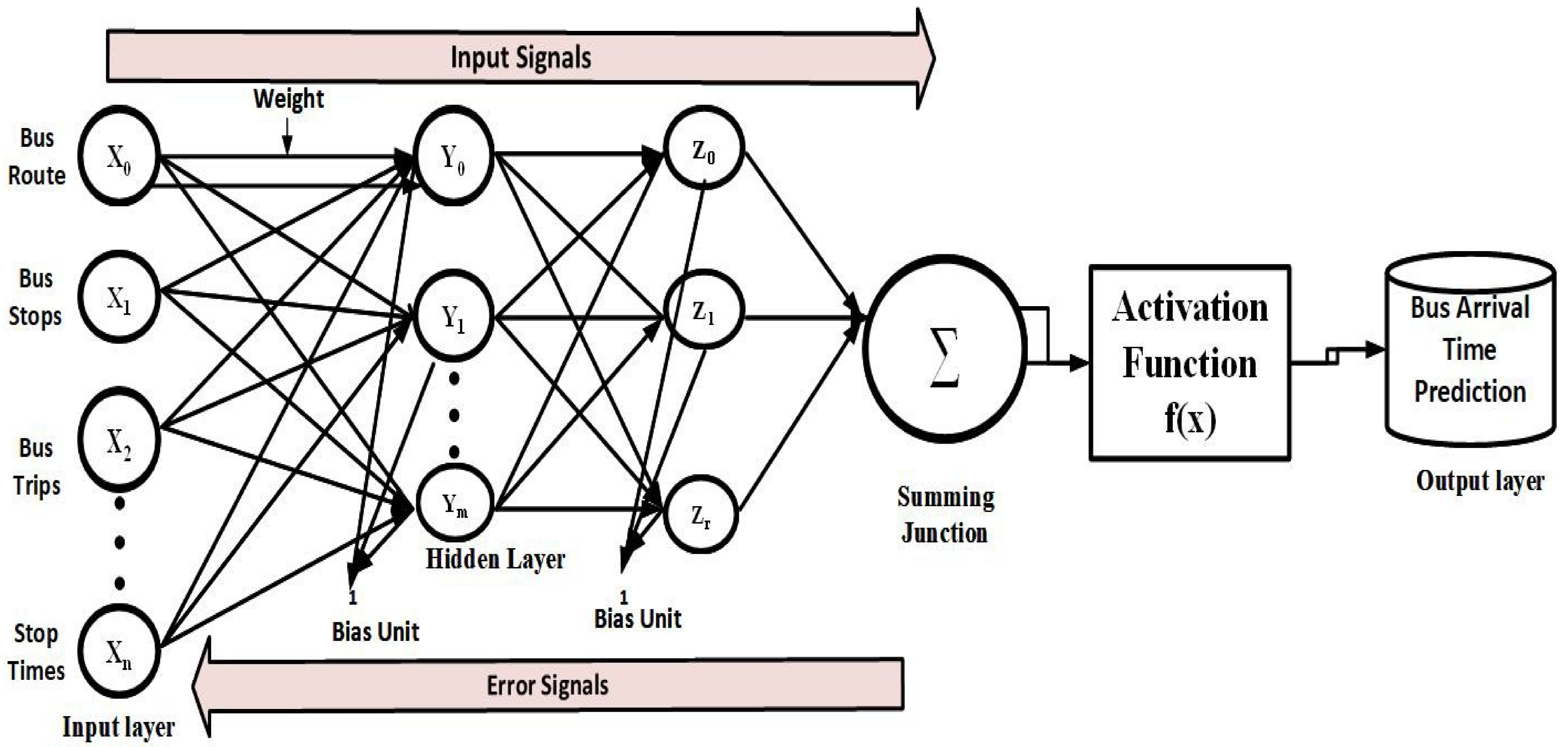
3.2. Bus Arrival Time Prediction Model

In the proposed system, we allocate data onto buses at each bus stop. The performance of data allocation highly depends upon coverage, mobility, and duration. For accurate modeling of data allocation, it is mandatory to know the accurate arrival time, leaving time, and dwell time of the bus at each bus stop. Thus, machine learning techniques are applied to develop a bus arrival time prediction model to give precise bus arrival information for applying proactive strategies for data dissemination. The provision of time and accuracy is important information for data allocation onto these buses for successful data transmission. The accurate information helps the controller to make a forwarding decision based upon the source and destination location and the route of the bus. An advanced neural network model is adopted using input features such as bus stops, bus routes, trips and many other features of a transport agency. Figure 2 shows the architectural diagram of the ANN algorithm w. It encompasses three layers, i.e., an input layer, a hidden layer, and an output layer.

• Input layer: This layer provides input to the neural network such as bus route, trips, and its corresponding metadata. The bus route consists of its name, id, and agency name. The bus trip is characterized by shape coordinates, trip id, route id, and direction. The first and last bus stop of each route is the source and destination stop, respectively. The input layer interacts with the data provided, accepts data in the form of signals or features. These features are then normalized to achieve better numerical precision when a mathematical model is applied at the hidden layer [42]. At this stage, small random values are initialized to the weights. The input layer just passes on the information to the hidden layer after adding weights without any computation. It is represented below. (

  Table 1. Variables used in the proposed model.

  Symbol	Meaning
  Xi	Input variables
  Wi	Weight
  f (θ)	ReLU function
  s	Speed of the bus
  tcd	Contact duration
  ten	Entering time
  tdw	Dwell time
  tex	Exit time
  d	Distance between RSU and bus
  rsp(t)	Received signal strength
  dre f	Reference distance
  Pr	Received power
  σ	Normal distribution random variable
  dex	Distance after t seconds of bus leaving
  nb	Background noise
  ρ	Mac efficiency
  µ	Throughput
  λmax	Max data rate

  )

  X_i = θ(X₁, X₂, ..., X_n)

  (1)
• Hidden layer: This layer accepts all the information from the input layer and feed-forward to all hidden layers to process it and forward it to the output layer. Next, this layer extracts all the features from the input layer and performs processing or training of the network with an activation function. The main motive of the activation function is to add nonlinearity into the network. There are many activation functions such as sigmoid, logistic, and hyperbolic tangent functions (tanh), ReLU, are the most common choices. In our model, the ReLU function is used as a rectifier unit for all input values and direct to (0, θ). This function is given by

  $$f\left(\theta \right)=max\left(0,\theta \right)$$

  (2)
  Here, the function outputs zero if the input values in the nonlinear function are negative or else equal to the value gives as input.
• Output layer: The output layer consists of results generated from previous layers. It updates errors as well as the weights associated with the connections (edges). The number of neurons in this layer corresponds to the output values of the problem. The neuron with n inputs calculates its output, as shown in Equation (3). As discussed above, all the input features are feed-forward, and then some bias weight is applied to the hidden layer, and finally, the output layer process the desired variables to be predicted.

  $$a=f({\displaystyle \sum }_{i=1}^n{W}_i{X}_i+b)$$

  (3)

  where X_i is the ith input
  W_i is the value of ith weight
  b is the bias, and f is an activation function.
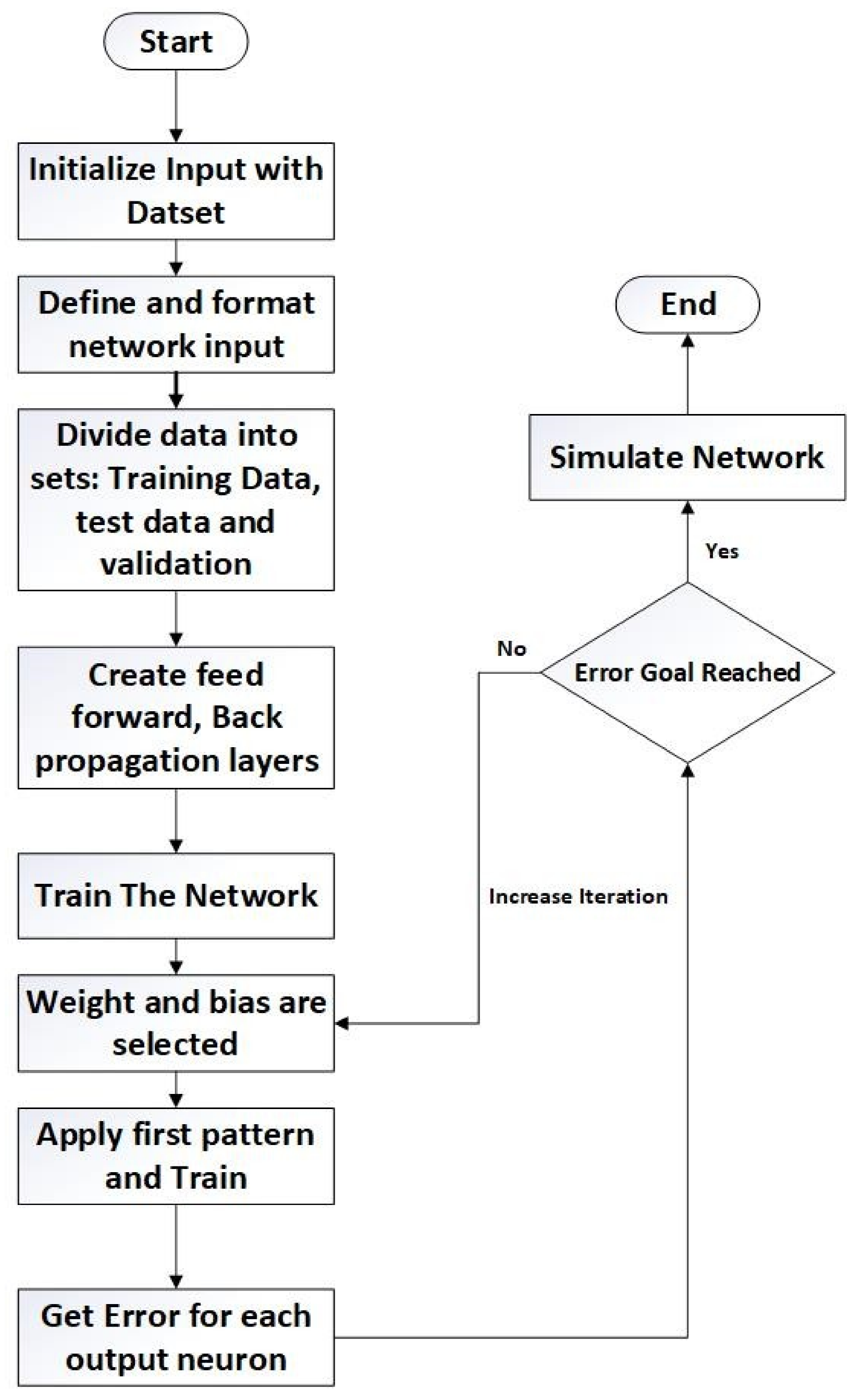
• Training, testing, and validation: Although the basic procedure of training any neural network is the same, however, the accuracy of the outcome relies on the features of input or output combinations. Therefore, it is highly important to validate a network to verify that training accuracy is sufficient or more iterations are required. During our ANN training algorithm as shown in Figure 3, we separate data input into two categories: one part is used to define the model, and the other part is used to validate the model. We use transport network input features as per time, date, stops, stop time. Next, we sort this input data to feed-forward to the input layer, the first 70% of data can be considered as training data to construct the model, and the next 30% is used for testing and validation.

The steps below will be followed by our ANN model to predict arrival time:

Step 1: Generating observations of the bus route: A random observation of all trips is to be generated and update zero for bus stops whose arrival time is to be predicted.

Step 2: Retrieve bus stop location details of all bus routes: Next, following our algorithm, we will fetch all the bus stops concerning their routes. For example, on the bus routes, there are a total of 29 bus stops. We will be calculating the bus arrival time for all these bus stops.

Step 3: Generate a symbolic formula and perform ANN model training: Our ANN model is accepting input as bus stop sequence (BS), the distance between two stops (d), the cumulative distance for the whole test trip CD_tt, the time between stops (T_s), arrival time in seconds (AT_s), speed (S), and cumulative travel time (CTT_s). Therefore, the initial symbolic formula description of the model to be fitted will be as.

X = (B_s + d_s + CD_tt + T_s + AT_s + S + CTT_s)^t

(4)

Step 4: Computing prediction and storing the predicted value: In the previous step, when a model is trained with sample data of a fixed route, ANN model results are used to predict bus arrival time for all other routes. These values will be stored in the predicted data frame and will be used for the comparison between actual and predicted arrival time. Similarly, Step 3 and Step 4 will be repeated for all the test trips.

Step 5: Performance metrics evaluations: We will consider the following performance metrics to estimate the results from the ANN model for all the predicted and actual arrival time values.

• Mean absolute percentage error (MAPE) = MAPE is defined as the average percentage difference between the observed value and the predicted value of bus arrival time. Where y_i = Predicted value, y₀ = observed value.

  $$MAPE=\frac{1}{n}{\displaystyle \sum }_i^n\frac{\left|y_i-y_0\right|}{y_0}\times 100\%$$

  (5)
• Symmetric mean absolute error (SMAPE) = It is an accuracy measure based on percentage (or relative) errors between the observed value and the predicted value.

  $$SMAPE=\frac{1}{n}{\displaystyle \sum }_i^n\frac{\left|y_i-y_0\right|}{(|y_i|+|y_0|)/2}\times 100\%$$

  (6)

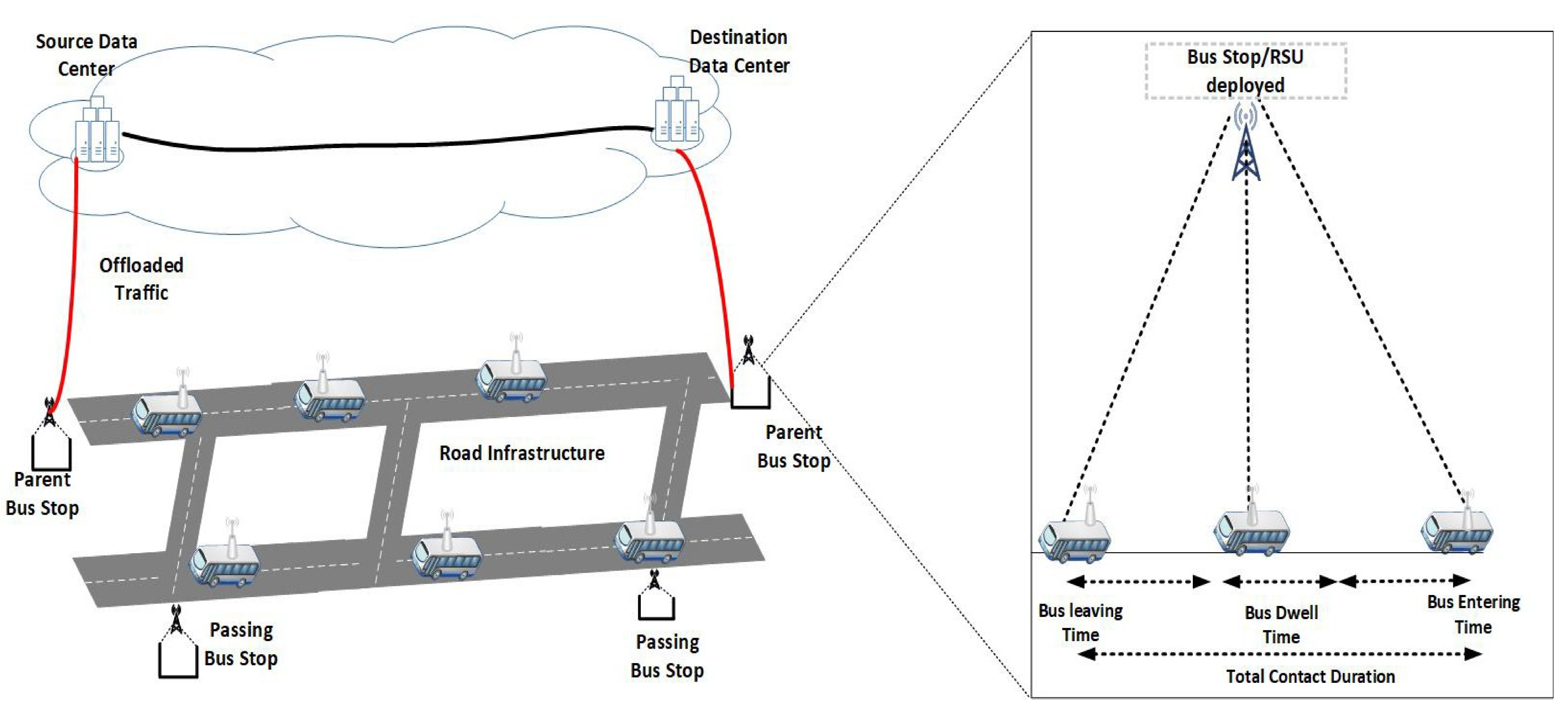
3.3. Data Offloading Model onto Buses

Next, after predicting the arrival time of the bus, we have better information about the time of the bus arrival at each bus stop to be into the ranges of RSU to get data to be allocated onto them. The offloading capacity of each bus stop depends upon two parameters. (1) contact duration, and (2) data throughput. We will first analyze the contact duration of buses, including entering, exiting time, and dwell time at each bus stops for data allocation. Each bus stops for a shorter period at the passing stop and a longer period at parent stops (source/destination). However, bus dwell time depends upon many factors such as passenger activity, time of day, route type, and bus floor. Moreover, all buses’ real-time information is periodically being sent to the base stations so that they can keep track of the vehicles and which ultimately helps to determine the link stability and data offloading at each bus stop. Data throughput can be obtained as a percentage of maximum data being transferred with respect to current bandwidth. To attain maximum efficiency in our proposed work, we will consider two types of stops, such as stopping stops and passing stops. Stopping stops further include all the stops, where buses stop for a longer or shorter duration, including parent stops (source or destination stops).We also assume that bus entering and exit speed will be equal as buses slow down while entering stops. Additionally, the location of RSU does not affect contact duration as it is placed exactly where the bus stops. Figure 4 gives a schematic overview of the operation to offload a large amount of delay-tolerant background data over the road infrastructure between two remote data centers using bus stops in between.

• Data offloading for stopping stops: Recall that the objective is to use public transport vehicles to carry large amounts of delay-tolerant data while reducing traffic load from existing infrastructure. All buses pass by bus stops, and data can be offloaded as per the dwell time, enter time, exit time, and contact duration of the bus into the range of the deployed RSU.

t_cd = t_en + t_dt + t_ex

(7)

where t_en, t_dt, t_ex, and t_cd are the bus entering time, dwell time, exit time, and contact duration at each bus stop, respectively. We assume that bus entering/exit speed is the same and gradually decreases/increases with speed (s) until it further reaches the next bus stop. We state the communication range (CR) for each bus while coming in contact with the RSU deployed at each bus stop as

d_ex = st² + v₀t + d

(8)

where d is the distance between the RSU deployed and the bus during stay time. d_ex is the distance after t seconds of the bus leaving the stop or from the range of deployed RSU. Bus stops at stopping stop, in this case, bus leaves a station from standstill situation and therefore v₀ = 0.

To calculate data throughput, it is important to know the received signal power (rsp). This depends upon the distance from the deployed RSU and the bus arrival or staying time. We will be calculating rsp(d) using the distance between RSU and log-normal shadowing path loss model as follows

rsp(d) = P_r − 10φ log(d_ex/d_{re f}) + σ

(9)

where P_r is the received power from RSU at reference distance d_{re f}, φ is the path loss component (PLE), σ is the normally distributed random variable. P_r can be further obtained by following

P_r = P_tr − 20log 4 ∗ π ∗ d_{re f}/λ

(10)

where P_tr is the transmitted power and λ is the signal wavelength in meters and can be obtained from λ = c/f, where c is the speed of light and f is the frequency. d is the distance from the RSU, and the bus and effective distance can be 2d, the diameter of the radius coverage area of RSU deployed at bus stops. Every bus will be in coverage as it starts entering at bus stops. Their data will start offloading at a distance from 0 to 2d meters. Moving further, received signal power rsp also depend upon the time (t), therefore considering d_{re f} = 1 m, rsp with respect for time is defined.

$$rsp\left(t\right)= P_r-10\phi \log \left(\frac{1}{2}s{t}^2+d\right)+ \sigma$$

(11)

We use the IEEE802.11 module as an interface to make a connection between the bus and RSU. The maximum throughput is calculated based upon signal-to-noise ratio SNR(db), which can be calculated as follows:

SNR(in db) = rsp(t) − n_b

(12)

where n_b is the background noise. Furthermore, SNR(db) based upon a time can be obtained as:

$$SNR\left(t\right)= P_r-n_b-10\phi \log \left(\frac{1}{2}s{t}^2+d\right)+ \sigma$$

(13)

The maximum bit rates λ^max rates are attained from MCS mapping tables bandwidth b_w based upon different frequencies (f), number of spatial streams (SS), and duration of the guard interval (GI).

∀snrⁱ ≤ snr(t) < snrⁱ⁺¹ → λ^max

(14)

where i = 0, 1, 2, …, 9 from MCS index to attain maximum bit rate and F is the mapping function. The throughput µ(en/ex) can be obtained from the maximum data rate (λ^max) and MAC efficiency (ρ).

µen/ex = λmaxρ

(15)

Hence, offloading capacity (O_c) is the sum of the capacity for stopping bus stop, or non-stopping bus stops as defined above as two different cases.

$$O_{stopping}= {\displaystyle \sum }_{i=1}^{N_{stp}}\left({\mu }_{st}^i\ast t_{st}^i+2{\displaystyle \sum }_{t=0}^{t_{max}^i}{\mu }_{en/ex}^i\ast \mathsf{\Delta }{t}^i\right)$$

(16)

where ${\mu }_{st}^i$ is the maximum throughput at stay time $t_{st}^i$ for all the stopping bus stops. Parent bus stops will also be considered under stopping bus stops. i is the range from 1 up to N number of stops (1 $\le i\le N_{stp}$ ) referring to all stops including parent stops.

3.4. Data offloading for Passing Stops

The bus just passes through the passing stop with a constant speed (i.e., s = 0), and there are no passengers to board at a bus stop. In this case, the bus comes in contact with any bus stop for a very short duration. Where time (t) is defined as

t = 2t_ps

(17)

where t_ps = d_ex/v_ps, v_ps is the velocity at the time of passing stops. Substituting values in (5), it is:

d_ex = v_ps ∗ t + d

(18)

Furthermore, to obtain received signal power again for passing stops is defined as

rsp(t) = P_r − 10φ log(v_ps ∗ t + d) + σ

(19)

The offloading efficiency of passing stop is

$$O_{passing}= 2{\displaystyle \sum }_{j=1}^{N_{ps}}{\displaystyle \sum }_{t=0}^{t_{max}^j}{\mu }_{ps}^j\ast \mathsf{\Delta }{t}^j$$

(20)

where j is the list of stops, where bus passes by (1 ≤ j ≤ N_ps).

3.5. Total Data Offloading for NESUDA

We have analyzed offloading efficiency for two different types of bus stops. If the bus stops for some time at any stopping bus stop, then we obtain offloading efficiency of stopping bus stop O_stopping from equation 16. On the other hand, if the bus just passes through any passing stop, then the offloading efficiency O_passing will be calculated from equation 20. The total offloading efficiency O(Total) of the public transport network can be acquired from the equation

O = O_stopping + O_passing

(21)

By substituting (16) and (20) into (21), we have

$$O\left(Total\right)= {\displaystyle \sum }_{i=1}^{N_{stp}}\left({\mu }_{st}^i\ast t_{st}^i+2{\displaystyle \sum }_{t=0}^{t_{max}^i}{\mu }_{en/ex}^i\ast \mathsf{\Delta }{t}^i\right)+2{\displaystyle \sum }_{j=1}^{N_{ps}}{\displaystyle \sum }_{t=0}^{t_{max}^j}{\mu }_{ps}^j\ast \mathsf{\Delta }{t}^j$$

(22)

4. Evaluation Results

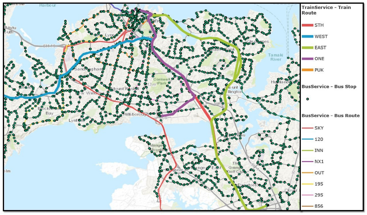
4.1. Case Study: Auckland Public Transport Network

We use the Auckland city public transportation system as an example to validate our proposed system. This data set allows us to study the spatial-temporal characteristics of the bus system to be utilized for data transmission. The AT map, as shown in Figure 5, clearly shows Auckland bus routes with their respective bus stops. We collected Auckland transport data sets from “Auckland Transport Open GIS data” resources. This is freely downloadable in general transit feed specification (GTFS) format.

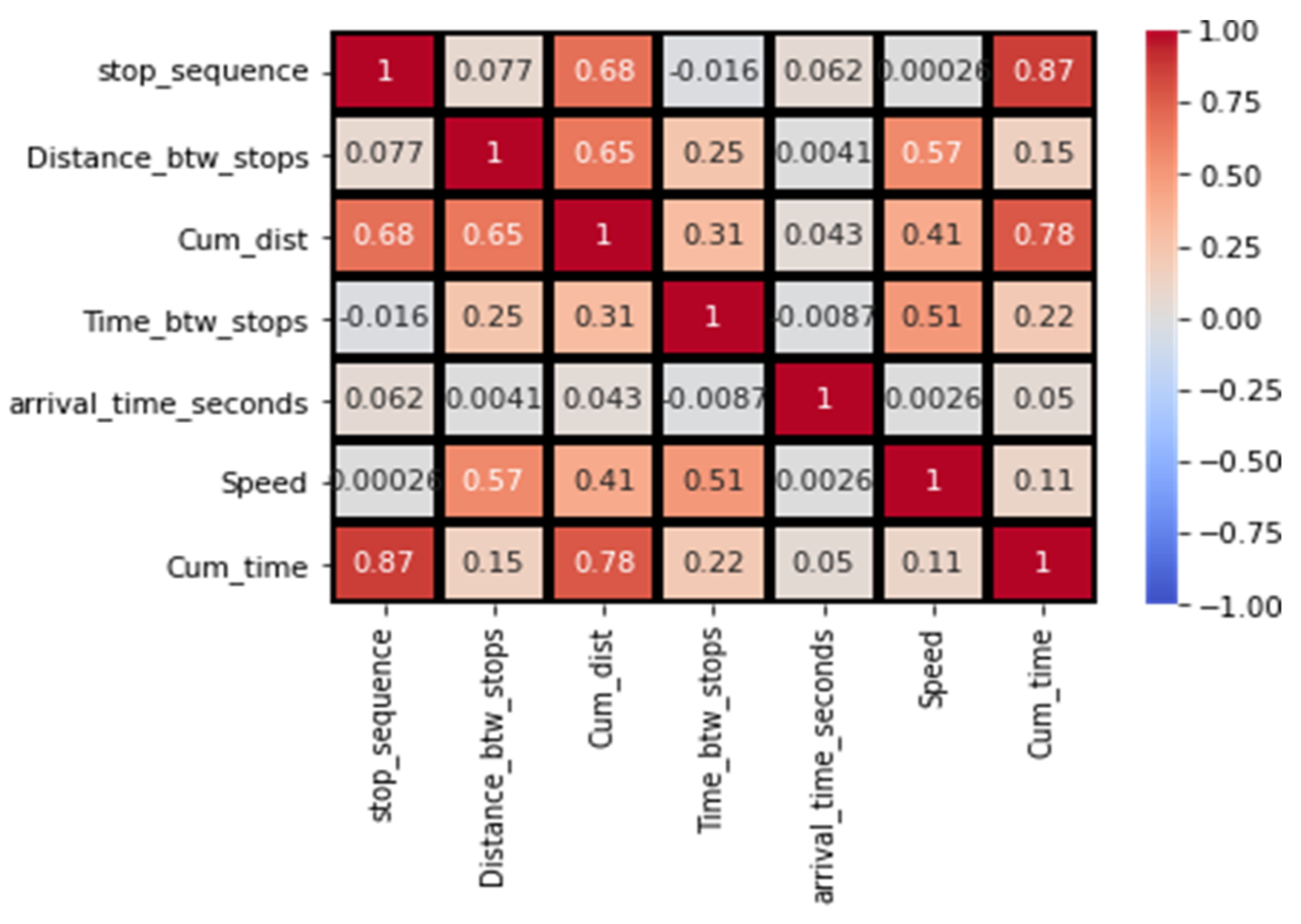
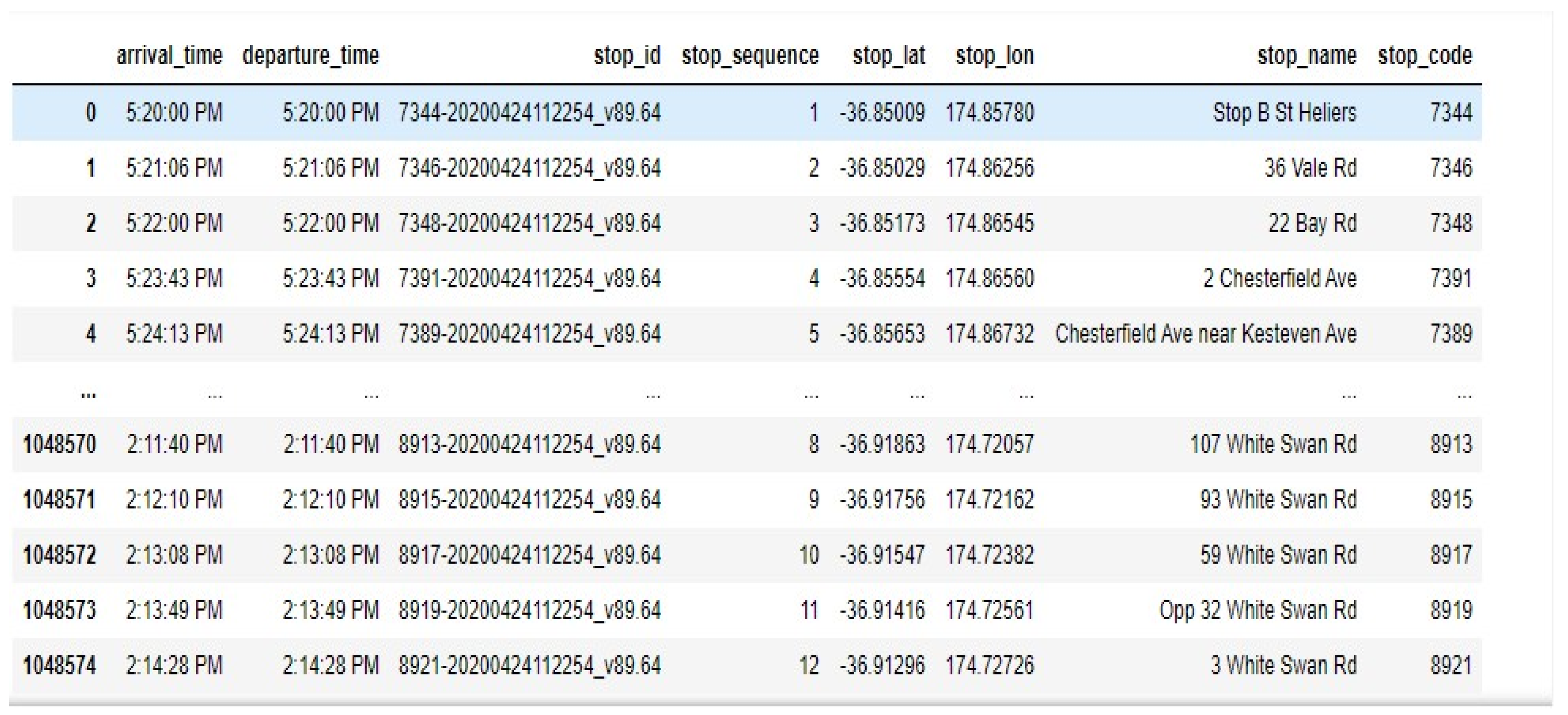
4.1.1. Data Preprocessing of Collected Dataset

The obtained dataset includes all the information related to buses and bus stops. It comprises the trip id of a bus, timestamp, longitude, and latitude of all the bus stops, etc. These data include trips over different routes with different directions, either upstream or downstream. The trips, stop_times, and routes dataset are the baseline dataset for the analysis to get details like scheduled arrival time and the departure time of all buses, fixed latitude and longitude positions of bus stops, which in turn helps to compute different data features for bus arrival time prediction.

• Calculating the distance between two bus stops

To evaluate bus arrival time, it is important to know the travel time and distance between two consecutive bus stops. There are many techniques available for calculating the distance between two bus stops. As defined in the description of the data set, the bus stop file contains its stop id along with longitude and latitude attributes. We use the well-known distance computation Haversine formula [43] to calculate distance as below:

$$D=2r arscin(\surd Havrsine({\varphi }_2-{\varphi }_1+\cos {\varphi }_1\cos {\varphi }_{2}Haversine\left({\lambda }_2-{\lambda }_1\right))$$

(23)

where D is the distance to be calculated, r is the radius of the earth, which is 6378.1 km, and φ₁, φ₂ implies the latitude of stop1 and stop 2. λ₁ and λ₂ denotes the longitude of stops 1 and 2.

2.

Calculating bus travel time between two bus service stops

The bus travel time is another feature to be calculated to help us with our bus arrival time prediction. An array of timestamp values is obtained from all the bus stops spots. Eventually, this feature from the stop time file will help to compute the travel time between consecutive bus stops and the cumulative time taken at each bus stop. Time value in this array is in the format of “HH:MM: SS”, so this array will be converted into seconds by the given formula.

Time (s) = HH × 3600 + MM × 60 + SS.

(24)

The array will be revised with these calculated times in seconds for each consecutive bus stop. To calculate the bus travel time for the current bus stop, the current time is subtracted from the next time. In some cases, the bus starting from the main bus stop (source) starts with some delay. This may be because of passengers boarding and delay in completing the existing trip. It was also seen that some buses start 1∼2 min ahead of the scheduled time from the source.

3.

Calculating speed between two bus service stops

Speed is another feature to extract to know the whole day journey of a route. It is being calculated as distance covered per unit of time. However, we will be concerned about the average speed over the linkages between all the bus stops of a bus route. With the extraction of this feature, we could calculate the delay in seconds that the bus is arriving early or late on a bus route. The negative value of delay implies that the bus is arriving late at a bus stop instead of the actual time, and the early arrival of the bus is being denoted by the positive value. The correlation matrix helps to understand the relationship between multiple features and attributes in the dataset to train our model. The correlation score value varies between 0 and 1, as shown in Figure 6. If there is a strong and perfect positive correlation, then the result is represented by a correlation score value of 0.9 or 1 or otherwise less.

4.

Testing and validation

To test and validate our ANN model on the AT network, we used 3 months of data from 20 April to 20 June. The collected data were converted to 1410 route segments with 1048574 trips in their operational times for each bus running along the route upstream and downstream. The total bus stops were 18,423 to be considered for RSU deployment. The AT training sample date is shown below in Figure 7. This is the ready data set used for testing and validation after applying preprocessing functions, removing unwanted data and null values. It is known as GTFS static and includes all the bus schedules and associated geographic information. This dataset is static and does not consider dwell time, passenger boarding, alighting, and other parameters. We used the first 70% as training data to construct the model, and the next 30% is used for testing and validation. We used a maximum of 500 iterations for our model. Of the testing set, 20% of the data set was taken as a validation test. This division has been used by many researchers [44] and helps to have better prediction results and minimum mean absolute percentage error (MAPE).

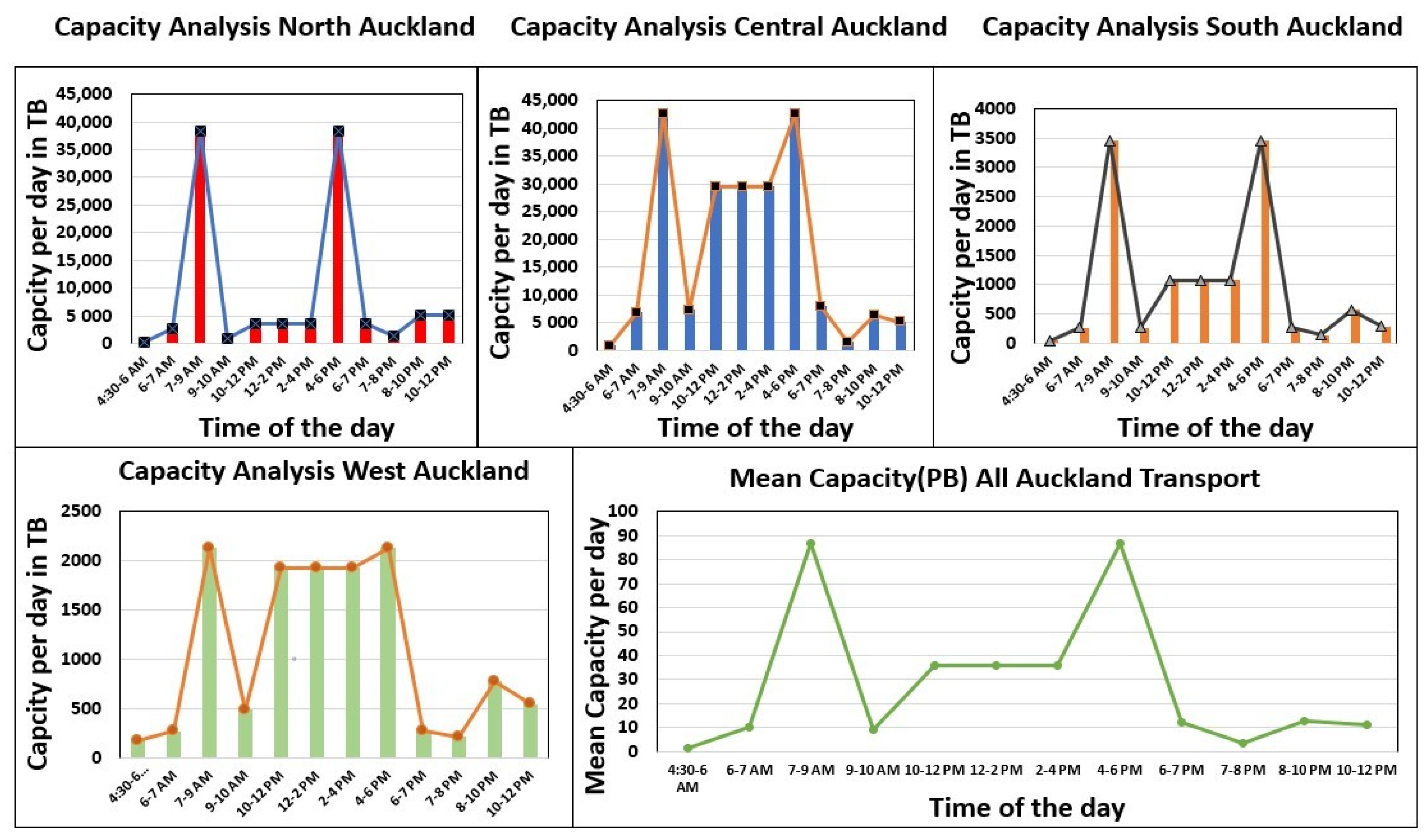
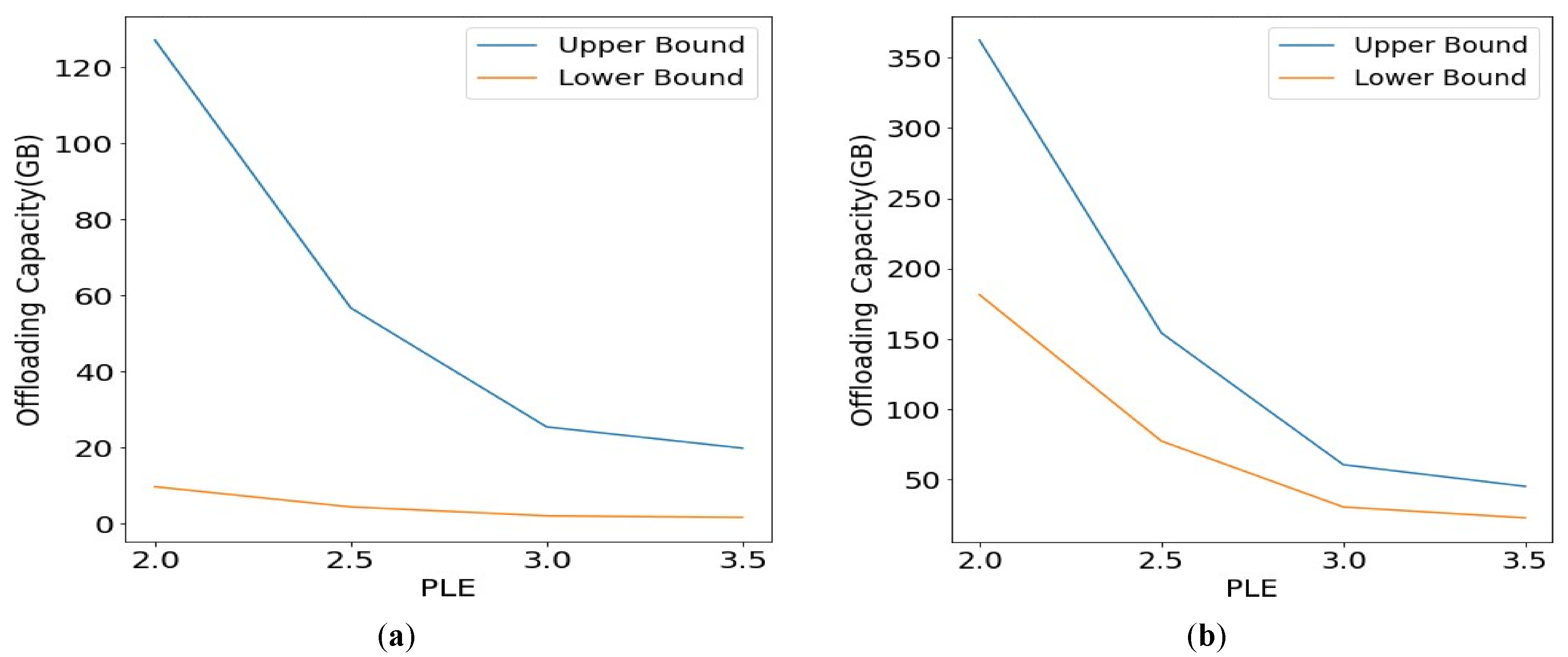
4.1.2. Auckland Transport Capacity Analysis

Our main aim was to effectively utilize the existing public transport for data dissemination. For this evaluation, we count all the possible routes of road network from sources to destinations. This study shows the benefits of using buses to carry data. To begin with, we first studied the potential transmission capacity of the Auckland region for one day during weekdays. We are considering all the bus services, which start at 4.30 a.m., including frequent services, local services, busway services, and connector services. Moreover, we have inbound and outbound services for a route, but with different bus stops. The frequency is an important factor impacting the data capacity for that time of day. We can see the increasing trend between 7 and 9 a.m. and 4–6 p.m. These are the peak times for the bus services with additional bus services scheduled during weekday days. We have calculated the bus services running during daytime hours, and we assume that each bus has a capacity to carry 100 GB, and based upon this, we calculated the capacity of all Auckland regions of different areas. We define the capacity c(i,j) as the maximum amount of data that can be transported from i to j by buses in a time frame as follows (in Mbit/s).

$$c\left(i,j\right)= B{s}_i{\displaystyle \sum }_{t\in i,j}{V}_t$$

(25)

where S_i is the storage capacity (in MBits) of every bus, B is the number of buses participating in carrying data with storage for particular demand between locations i and j in the time T (in hours), and V_t is the number of buses per unit of time going from i to j. The overall capacity of all buses per day for north Auckland is 106,031.8 TB, which is massive and can be utilized efficiently to carry data. For example, video surveillance data get captured by cameras, and the Auckland bus service can collect data from different regions to efficiently carry that data to the transport center for further analysis. As these data are not urgent and can be delayed up to a few hours. As said before, Auckland central is the hub of the Auckland region. The bus services start from Auckland CBD and go in all directions. In this way, the Auckland central area has more capacity to disseminate data as it has more capacity for the whole day. The average capacity of Auckland central per day is 210,226.8 TB.

In South and West Auckland, there are in total 107 and 138 bus services, which run all over the day. There is a train service in the south, which starts from Auckland central and covers central to the south covering many suburbs. Therefore, the overall capacity of all buses per day in south Auckland is 12,037.2 TB. As shown in Figure 8, among all of the four regions of Auckland, the North and Central Auckland bus service haves more capacity in comparison with South and West Auckland to disseminate data all over Auckland just because of the scheduled train services in that area. The mean capacity of all Auckland transport bus service is 85,274.025 TB in total, which demonstrates the great potential of using our proposed for data dissemination. These bus systems can participate in data dissemination from one place to another which can help to leverage the heavy data burdens on the traditional telecommunication infrastructure as well as best utilize the public transport for added value services in the big data era.

4.2. Auckland Transport Test Trips

To evaluate our bus arrival time prediction model, three test trips were conducted for different routes of the Auckland public transport network.

Table 2. Set of test trips with the number of bus stops.

Test Trip	Number of Bus Stops
Test trip 744	29
Test trip 141	32
Test trip 70	46

is presented to demonstrate the set of test trips with random bus trips that were created by the algorithm for bus route 744, 141, and 70 runs in the afternoon hours of the day. The ANN model was trained and tested with such random observations, and then MAPE and SMAPE metrics were estimated for actual arrival time and predicted bus arrival time values from the ANN model. Figure 9, Figure 10 and Figure 11 illustrate the selected bus route with bus stops (snapshot from the moovit app). This ready data set is used to train the model to predict arrival time at each bus stop in offline mode.

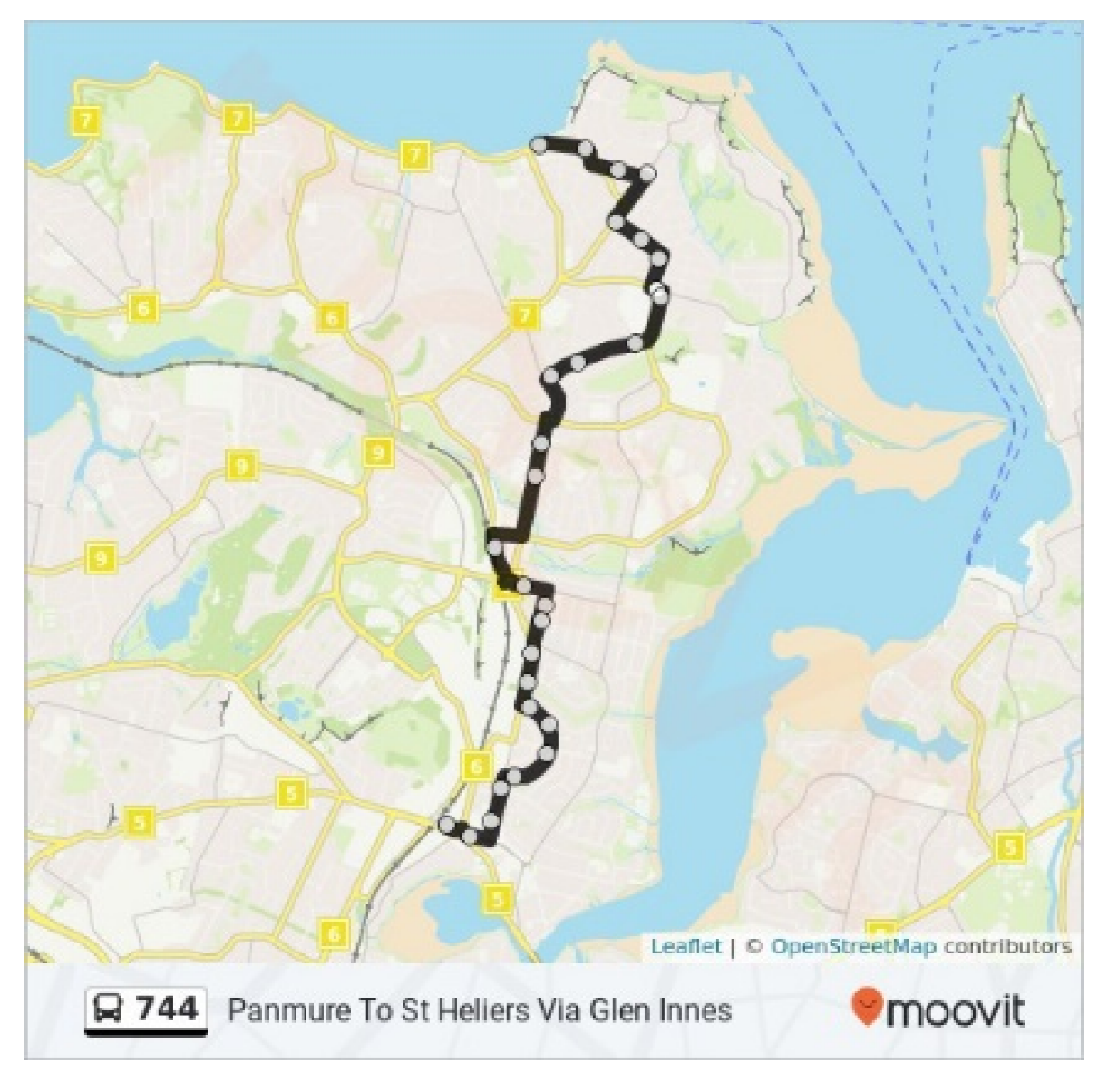
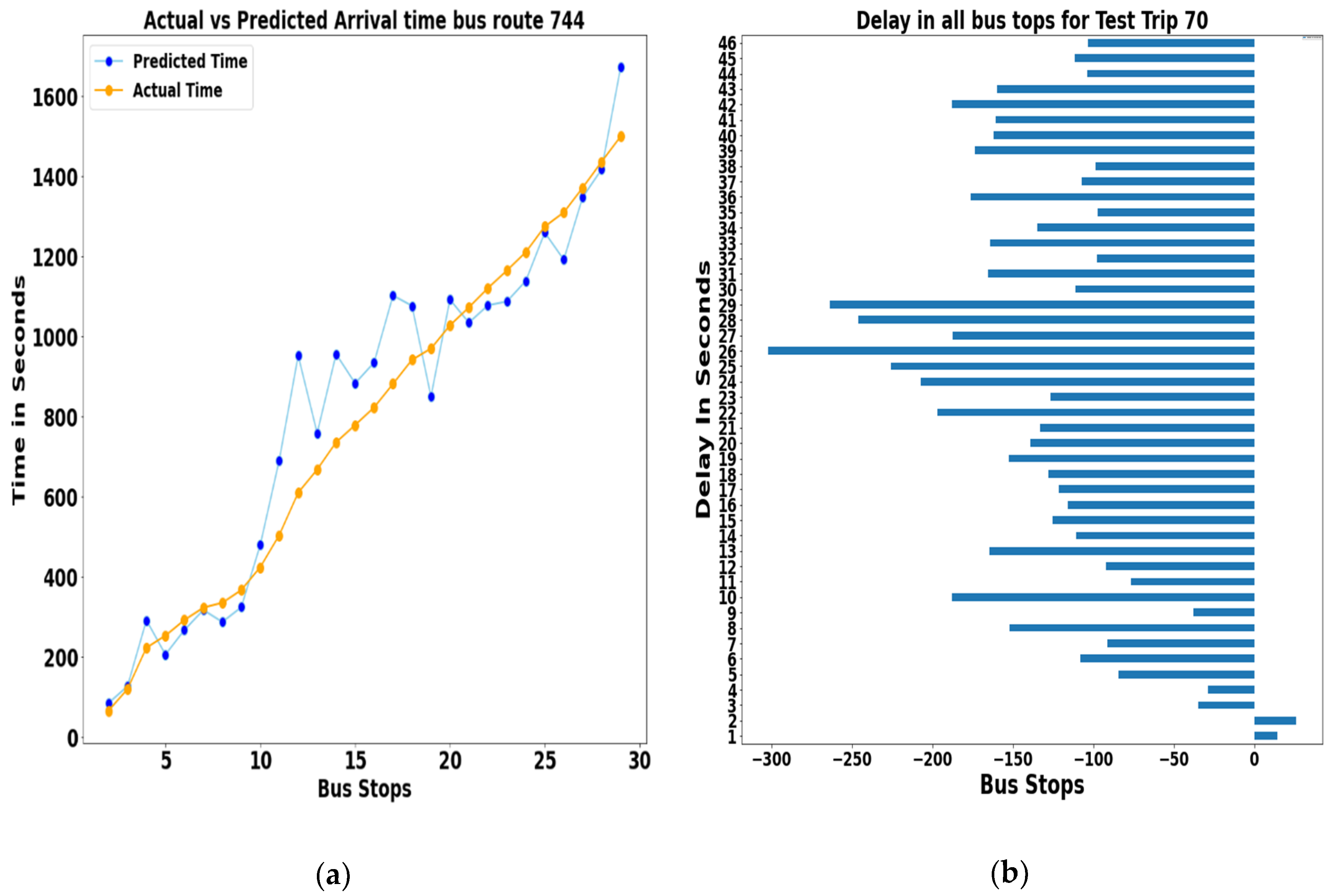
• Test Trip 744: The testbed selected as a sample is the Auckland Transport bus route 744. Which is one of Auckland’s central services and connects St Heliers To Panmure via Glen Innes, considering downstream direction covering 29 stops with trip duration for 25 min and length of route of 7 km in between Stop 1 and Stop 29. Figure 12a illustrates the behaviors of actual and predicted bus arrival times at each bus stop after validation of the neural network algorithm. On the x-axis, the bus stop numbers are plotted, starting from the target station of each testing sample up to the last destination of the bus trip. On the y-axis, the arrival time (seconds) taken at which a bus reaches any bus stops on its route is plotted. The trained algorithm trend proves that there is a slight difference at a few bus stops between actual and predicted arrival times. Figure 12b represents the delay (seconds) to reach each bus stop. The negative value represents that the bus is arriving late at each bus stop. On the other site, positive values indicate the early arrival of buses at each stop, which ultimately represents the variation in bus arrival time. We are considering buses to carry data with delay-tolerant features. Therefore, this much delay variation is acceptable to use buses as another communication mode.
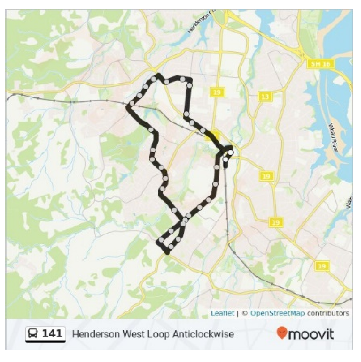
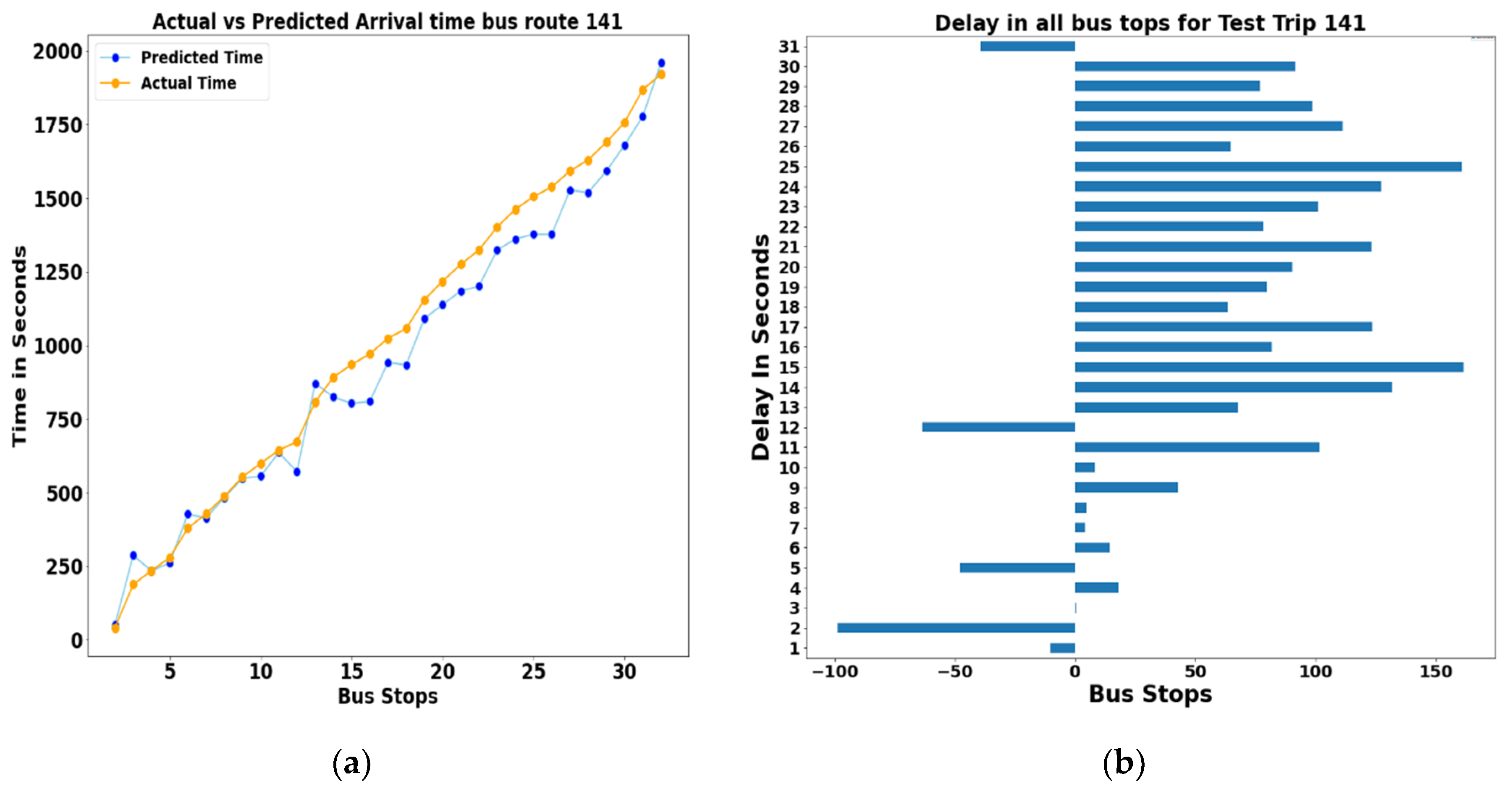
• Test Trip 141: The next test trip selected is number 141, which is called Henderson West Loop Anticlockwise. This trip has 32 stops and covers the whole journey in approximately 33 min. The bus departs from Stop A Henderson Interchange and finishes at Stop B Henderson Interchange. The operating hours for this bus are from 05:15 to 23:15 every day, including weekend hours from 06:38 to 23:08. Same way as the previous trip, Figure 13a illustrates that there is variation between predicted and actual arrival time. However, Figure 13b clearly shows that the bus is arriving early most of the time at each stop except 5 or 6 bus stops, which clearly states that we can use public transport as another communication mode with delay-tolerant features.
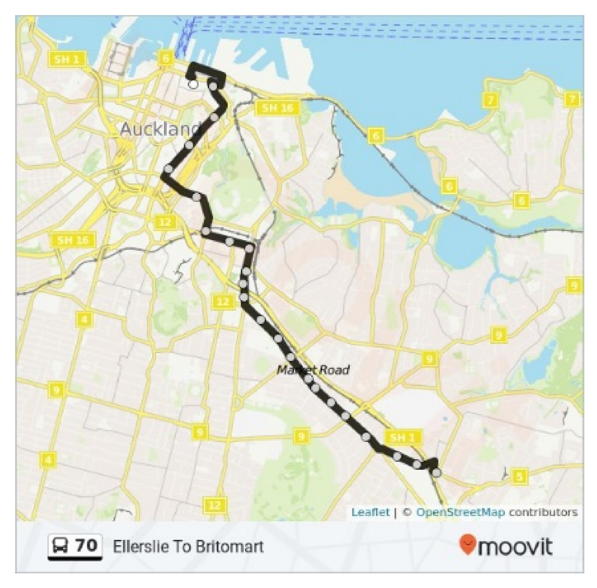
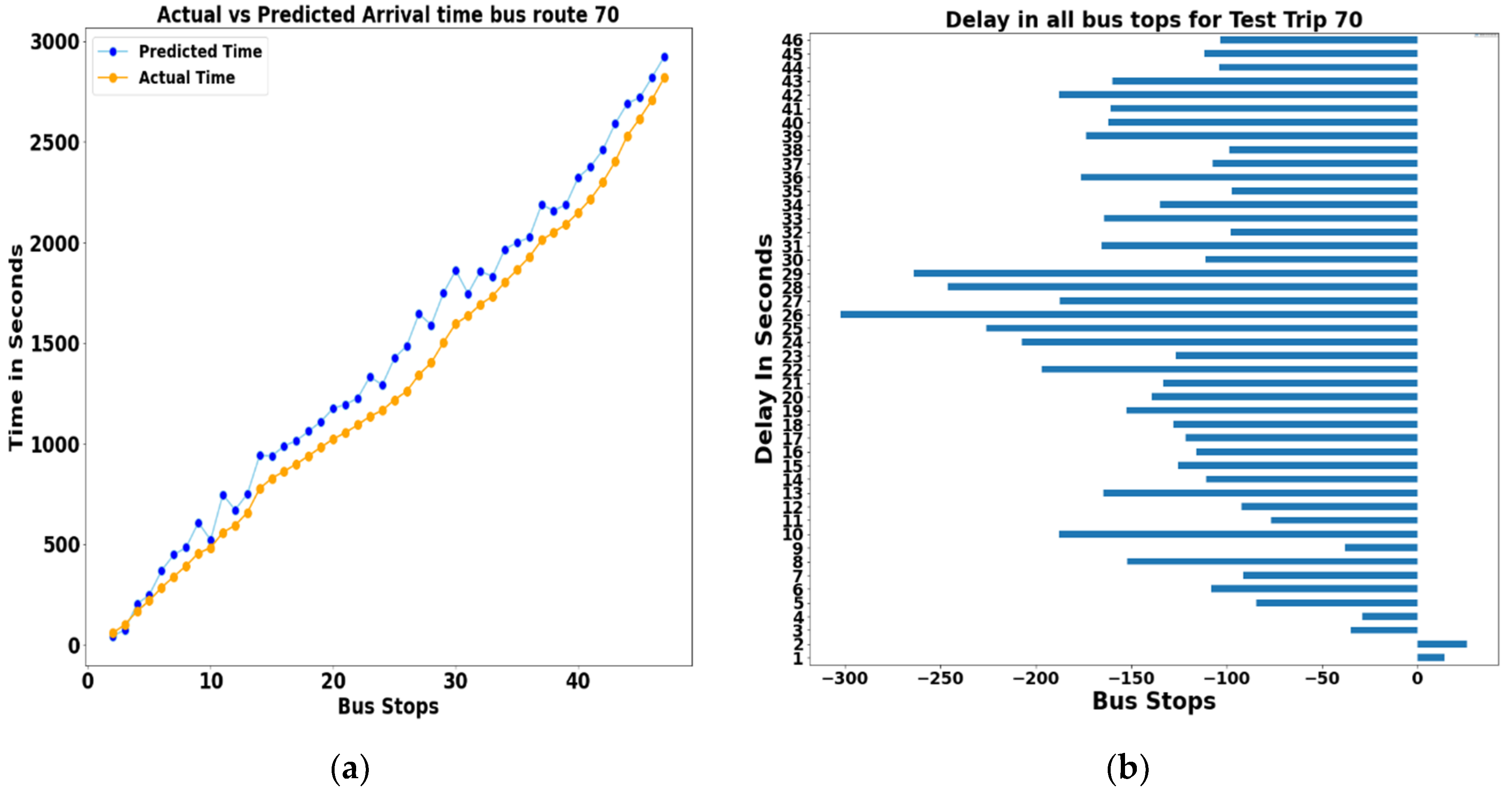
• Test Trip 70: This test trip 70 starts from 56 Customs St east near Britomart and ends in Stop A Botany town center. This trip covers a total of 46 stops in approximately 58 min. This bus route is operational every day, and the first journey starts at 00:05 and ends at 23:50 every weekday, and on the weekend, it begins at 06:15 am and ends at 23:35. Similarly, Figure 14a illustrates the trend of actual and predicted bus arrival time at each bus stop. This route shows that actual and predicted arrival time is different on each bus stop and never on the scheduled time. In Figure 14b, delay(seconds) represents all the negative values and implies that the bus is late at each bus stop.

Table 3. Mean absolute percentage error (MAPE) value and its interpretations.

MAPE	Interpretation
<10	Highly accurate forecasting
10–20	Good forecasting
20–50	Reasonable forecasting
>50	Inaccurate forecasting

presents containing typical MAPE interpretation to analyze our ANN model results.

Table 4. Calculated MAPE and symmetric mean absolute error (SMAPE) error values.

Test Trip	MAPE	SMAPE
Test Trip 744	14.98	0.1447
Test Trip 141	13.34	0.1551
Test Trip 70	19.83	0.0687

is created to show the MAPE and SMAPE values calculated for each test trip, and the lowest MAPE and SMAPE that were estimated for the model was observed for test case trip 744 with 13.91% and 0.1477 error, respectively.

Algorithm 1: Data Allocation onto Buses
Input:   s: Source location, d: Destination location, t: Stay Time, b: Available bus
Output:  Status Message
1.  while true do
2.    m←wait(s);	// wait for message from nodes
3.    move (φs, λs);	// Reach near source location or bus-stop
4.    Available (b, t)	// Check for available bus and stay time
5.    Upload (s, b)	// Upload data onto bus
6.    move (φd, λd);	// Reach near destination location or bus-stop
7.    download (b, d)
8.    If !valid() then
9.     Notify (d)
10.   end if
11.  end while

To evaluate our proposed model, we already used the AT data set. We assume that an IEEE802.11ac-based WLAN is dedicated for data allocation at each bus stop with different bandwidths such as 20 MHz, 40 MHz, 80 MHz, and 160 MHz as per algorithm 1 This represents the data allocation from the source until the destination for the broadcast job. The data gets allocated onto available buses near-the source location and download at the near destination location. Finally, a data integrity check is done after merging data at the destination stop. We used different parameters to calculate offloading efficiency for stopping stops and passing stops. We will be considering 20 MHZ as the worst-case scenario to evaluate path loss for distance and normal distribution for buses when they start approaching bus stops and leave bus stops. Assuming the stay time of the bus between 20 s as the minimum guaranteed value and can increase up to 120 s. The velocity of buses at the entering or leaving time will be considered as 20 m/s. To evaluate the performance, we will consider different values of PLE to evaluate the performance for different environmental conditions at each bus stop with the noise level value to be −90 db. Figure 15 and Figure 16 show the path loss and distribution of vehicles obtained from Equation (9). Path loss increases with the distance and reaches up to 80 db.

The stay time of buses to be in coverage of the RSU is proportional to the speed of the vehicle. Therefore, the offloading data rate, as shown in Figure 17, depends upon the bus density and the speed of the bus while entering/leaving the bus stop. We plot the CDF of stay time at each passing stop and end-stop, as shown in Figure 18 and Figure 19. It shows that more than 50% of the buses stop at the end stop for more than 9 min. Figure 20 shows the SNR versus time for different PLE values and changes as per timings. We applied the RBAR method to theoretically estimate the maximum data throughput plotted in Figure 21 for the time to be in coverage of RSU as defined in equation 12. To illustrate the offloading capacity of upper bound and lower bound for different environments for different values for the transmitter is shown in Figure 22. For the upper bound, we assumed GI = 400 ns, 3 spatial streams, and 160 MHz channel, and for the lower band, 1 spatial stream, GI = 800 ns, and 20 MHz bandwidth. For example, with PLE = 2.5, we can achieve up to 60 GB offloading capacity for passing stop and 160 GB for stopping stop. By employing new standards, we can achieve more capacity as per each stopping station with maximum data rates.

In our previous work [45], we defined the energy consumption model for traditional networks and public transport networks. We evaluated the energy cost while transferring data using traditional networks or public transport networks from one place to another. As per our case study, we will calculate energy consumption to send data from different locations of Auckland using both networks. For example, while sending data from Auckland CBD to Henderson, there are two possible networks, and the distance is 17 km. The bandwidth to upload/download data using the core network will be considered as b_up and b_down. However, while using a bus network for data dissemination, the weight of the package is appx 0.95 (2 TB) and αdiesel as a constant with value 38, 290, 237.52 J/L to convert fuel volume into liters and joules.

Table 5. Energy cost parameters of Auckland city.

From	To	LAN	Edge Routers	Core Routers	bup	bdown	Distance (km)
Auckland CBD	Henderson	6	2	5	0.1	0.1	17
Manukau	Albany	13	2	15	0.1	1.0	39
Auckland CBD	Danemora	6	2	3	0.1	10.0	23
Manukau	Auckland CBD	11	2	3	1.0	1.0	30
Auckland CBD	Albany	8	2	14	1.0	1.0	18

gives a detailed description of the energy parameters used as per the distance in each location. We plot the energy consumption value as per different values of the data volume and distance in Figure 22 and Figure 23 The results show that our system will make an energy-efficient network selection in comparison with a traditional network.

5. Conclusions and Future Work

This paper exploits the existing road infrastructure, including public transport networks and utilizes them to disseminate data to overcome the limitations of conventional wired/wireless networks. To determine the scheduled movement of moving buses, we used the Auckland Transport case study to analyze their patterns. An advanced neural network algorithm was developed to predict bus arrival time prediction at each bus stop for each route. Computed features like distance traveled, demand characteristics, and time of day, average speed, travel time between bus stops were obtained from the Auckland Transport data set. As the available data were limited and historical, some assumptions were made for data processing to create input to train our model, and some data points were ignored because of errors and duplicates. Since the methodology used to develop all predictions is the same for all test trips, their MAPE and SMAPE errors are similar and can be presented in a range. Based on these performance metrics, our ANN model proves that there exists a delay in the actual and predicted arrival time of the bus. However, we can utilize them efficiently to disseminate data with delay-tolerant features. This difference can help to estimate the realistic arrival time of the bus to allocate data as per destination and the route. The offloading capacity is analyzed for each stop and terminal and proves that the public transport network can be utilized efficiently for data dissemination with significant savings of energy. We will study how to adapt the network selection decision between the traditional Internet network and our proposed transportation system-based data dissemination network in our future work for guaranteed delivery of data.

References

1. Cisco Systems. Cisco Visual Networking Index: Global Mobile Data Traffic Forecast Update, 2017–2022; Cisco: San Jose, CA, USA, 2019. [Google Scholar]
2. Liu, J.; Wan, J.; Zeng, B.; Wang, Q.; Song, H.; Qiu, M. A scalable and quick-response software defined vehicular network assisted by mobile edge computing. IEEE Commun. Mag. 2017, 55, 94–100. [Google Scholar] [CrossRef]
3. Smith, G.J.; Bennett Moses, L.; Chan, J. The challenges of doing criminology in the big data era: Towards a digital and data-driven approach. Br. J. Criminol. 2017, 57, 259–274. [Google Scholar] [CrossRef]
4. You, C.; Huang, K.; Chae, H.; Kim, B.H. Energy-efficient resource allocation for mobile-edge computation offloading. IEEE Trans. Wirel. Commun. 2016, 16, 1397–1411. [Google Scholar] [CrossRef]
5. Ekbatanifard, G.; Rajabi, M. An energy efficient data dissemination scheme for distributed storage in the internet of things. Comput. Knowl. Eng. 2017, 1, 1–8. [Google Scholar]
6. Chahal, M.; Harit, S. Network selection and data dissemination in heterogeneous software-defined vehicular network. Comput. Netw. 2019, 161, 32–44. [Google Scholar] [CrossRef]
7. Li, S.; Zhai, D.; Du, P.; Han, T. Energy-efficient task offloading, load balancing, and resource allocation in mobile edge computing enabled IoT networks. Sci. China Inf. Sci. 2019, 62, 29307. [Google Scholar] [CrossRef] [Green Version]
8. Pham, X.Q.; Nguyen, T.D.; Nguyen, V.; Huh, E.N. Joint node selection and resource allocation for task offloading in scalable vehicle-assisted multi-access edge computing. Symmetry 2019, 11, 58. [Google Scholar] [CrossRef] [Green Version]
9. Li, M.; Si, P.; Zhang, Y. Delay-tolerant data traffic to software-defined vehicular networks with mobile edge computing in smart city. IEEE Trans. Veh. Technol. 2018, 67, 9073–9086. [Google Scholar] [CrossRef]
10. Hu, L.; Liu, A.; Xie, M.; Wang, T. UAVs joint vehicles as data mules for fast codes dissemination for edge networking in smart city. Peer-Peer Netw. Appl. 2019, 12, 1550–1574. [Google Scholar] [CrossRef]
11. Singh, P.; Kaur, A.; Kumar, N. A reliable and cost-efficient code dissemination scheme for smart sensing devices with mobile vehicles in smart cities. Sustain. Cities Soc. 2020, 62, 102374. [Google Scholar] [CrossRef]
12. Poulliat, C. Mobile Data Offloading via Urban Public Transportation Networks. Ph.D. Thesis, Institut de Recherche en Informatique de Toulouse, INPT, Toulouse, France, 2017. [Google Scholar]
13. Han, Q.; Liu, K.; Zeng, L.; He, G.; Ye, L.; Li, F. A Bus Arrival Time Prediction Method Based on Position Calibration and LSTM. IEEE Access 2020, 8, 42372–42383. [Google Scholar] [CrossRef]
14. Wang, T.; Li, P.; Wang, X.; Wang, Y.; Guo, T.; Cao, Y. A comprehensive survey on mobile data offloading in heterogeneous network. Wirel. Netw. 2019, 25, 573–584. [Google Scholar] [CrossRef]
15. Lee, K.; Lee, J.; Yi, Y.; Rhee, I.; Chong, S. Mobile data offloading: How much can WiFi deliver? IEEE/ACM Trans. Netw. 2012, 21, 536–550. [Google Scholar] [CrossRef]
16. Mehmeti, F.; Spyropoulos, T. Performance analysis of mobile data offloading in heterogeneous networks. IEEE Trans. Mob. Comput. 2016, 16, 482–497. [Google Scholar] [CrossRef]
17. Barone, R.E.; Giuffrè, T.; Siniscalchi, S.M.; Morgano, M.A.; Tesoriere, G. Architecture for parking management in smart cities. IET Intell. Transp. Syst. 2013, 8, 445–452. [Google Scholar] [CrossRef]
18. Liu, H.; Xu, H.; Yan, Y.; Cai, Z.; Sun, T.; Li, W. Bus Arrival Time Prediction Based on LSTM and Spatial-Temporal Feature Vector. IEEE Access 2020, 8, 11917–11929. [Google Scholar] [CrossRef]
19. Wang, Z.; Zhong, Z.; Zhao, D.; Ni, M. Bus-based cloudlet cooperation strategy in vehicular networks. In Proceedings of the 2017 IEEE 86th Vehicular Technology Conference (VTC-Fall), Toronto, ON, Canada, 24–27 September 2017; IEEE: Piscataway, NJ, USA, 2017; pp. 1–6. [Google Scholar]
20. Ahmad, A. Utilizing Public Transport Networks for Bulk Data Transfer; University in Helsinki: Helsinki, Finland, 2019. [Google Scholar]
21. Baron, B.; Spathis, P.; Rivano, H.; de Amorim, M.D. Offloading massive data onto passenger vehicles: Topology simplification and traffic assignment. IEEE/ACM Trans. Netw. 2016, 24, 3248–3261. [Google Scholar] [CrossRef]
22. Malik, A.W.; Mahmood, I.; Ahmed, N.; Anwar, Z. Big data in motion: A vehicle-assisted urban computing framework for smart cities. IEEE Access 2019, 7, 55951–55965. [Google Scholar]
23. Kanwal, M.; Malik, A.W.; Rahman, A.U.; Mahmood, I.; Shahzad, M. Sustainable vehicle-assisted edge computing for big data migration in smart cities. IEEE Internet Things J. 2019, 7, 1857–1871. [Google Scholar] [CrossRef]
24. Komnios, I.; Kalogeiton, E. A DTN-based architecture for public transport networks. Ann. Telecommun. 2015, 70, 523–542. [Google Scholar] [CrossRef]
25. Bendouda, D.; Rachedi, A.; Haffaf, H. Programmable architecture based on software defined network for internet of things: Connected dominated sets approach. Future Gener. Comput. Syst. 2018, 80, 188–197. [Google Scholar] [CrossRef]
26. Teng, H.; Liu, Y.; Liu, A.; Xiong, N.N.; Cai, Z.; Wang, T.; Liu, X. A novel code data dissemination scheme for Internet of Things through mobile vehicle of smart cities. Future Gener. Comput. Syst. 2019, 94, 351–367. [Google Scholar] [CrossRef]
27. Dias, D.S.; Costa, L.H.M.; de Amorim, M.D. Data offloading capacity in a megalopolis using taxis and buses as data carriers. Veh. Commun. 2018, 14, 80–96. [Google Scholar] [CrossRef]
28. Hui, Y.; Su, Z.; Luan, T.H. Collaborative content delivery in software-defined heterogeneous vehicular networks. IEEE/ACM Trans. Netw. 2020, 28, 575–587. [Google Scholar] [CrossRef]
29. Naseer, S.; Liu, W.; Sarkar, N.I.; Chong, P.H.J.; Lai, E.; Ma, M.; Prasad, R.V.; Danh, T.C.; Chiaraviglio, L.; Qadir, J.; et al. A sustainable marriage of telcos and transp in the era of big data: Are we ready? In International Conference on Smart Grid Inspired Future Technologies; Springer: Berlin/Heidelberg, Germany, 2018; pp. 210–219. [Google Scholar]
30. Naseer, S.; Liu, W.; Sarkar, N.I. Energy-Efficient Massive Data Dissemination through Vehicle Mobility in Smart Cities. Sensors 2019, 19, 4735. [Google Scholar] [CrossRef] [Green Version]
31. Naseer, S.; Liu, W.; Sarkar, N.I.; Chong, P.H.J.; Lai, E.; Prasad, R.V. A sustainable vehicular based energy efficient data dissemination approach. In Proceedings of the 2017 27th International Telecommunication Networks and Applications Conference (ITNAC), Melbourne, Australia, 22–24 November 2017; IEEE: Piscataway, NJ, USA, 2017; pp. 1–8. [Google Scholar]
32. Munjal, R.; Liu, W.; Li, X.J.; Gutierrez, J.; Furdek, M. Sustainable Crowdsensing Data Dissemination Using Public Vehicles. In Crowd Assisted Networking and Computing; CRC Press: Boca Raton, FL, USA, 2018; pp. 77–110. [Google Scholar]
33. Munjal, R.; Liu, W.; Li, X.J.; Gutierrez, J.; Furdek, M. Sustainable massive data dissemination by using software defined connectivity approach. In Proceedings of the 2017 27th International Telecommunication Networks and Applications Conference (ITNAC), Melbourne, Australia, 22–24 November 2017; IEEE: Piscataway, NJ, USA, 2017; pp. 1–6. [Google Scholar]
34. Munjal, R.; Liu, W.; Li, X.J.; Gutierrez, J.; Chong, P.H.J. Telco asks transp: Can you give me a ride in the era of big data? In Proceedings of the 2017 IEEE Conference on Computer Communications Workshops (INFOCOM WKSHPS), Atlanta, GA, USA, 1–4 May 2017; IEEE: Piscataway, NJ, USA, 2017; pp. 766–771. [Google Scholar]
35. Manasseh, C.; Sengupta, R. Predicting driver destination using machine learning techniques. In Proceedings of the 16th International IEEE Conference on Intelligent Transportation Systems (ITSC 2013), The Hague, The Netherlands, 6–9 October 2013; IEEE: Piscataway, NJ, USA, 2013; pp. 142–147. [Google Scholar]
36. Patnaik, J.; Chien, S.; Bladikas, A. Estimation of bus arrival times using APC data. J. Public Transp. 2004, 7, 1. [Google Scholar] [CrossRef] [Green Version]
37. Zhao, X.; Yang, K.; Chen, Q.; Peng, D.; Jiang, H.; Xu, X.; Shuang, X. Deep learning based mobile data offloading in mobile edge computing systems. Future Gener. Comput. Syst. 2019, 99, 346–355. [Google Scholar] [CrossRef]
38. Chen, M.; Liu, X.; Xia, J.; Chien, S.I. A dynamic bus-arrival time prediction model based on APC data. Comput. Aided Civ. Infrastruct. Eng. 2004, 19, 364–376. [Google Scholar] [CrossRef]
39. Zhang, Z.; Wang, Y.; Chen, P.; He, Z.; Yu, G. Probe data-driven travel time forecasting for urban expressways by matching similar spatiotemporal traffic patterns. Transp. Res. Part C Emerg. Technol. 2017, 85, 476–493. [Google Scholar] [CrossRef]
40. Suk, H.I. An introduction to neural networks and deep learning. In Deep Learning for Medical Image Analysis; Elsevier: Amsterdam, The Netherlands, 2017; pp. 3–24. [Google Scholar]
41. Saki, M.; Abolhasan, M.; Lipman, J. A Big Sensor Data Offloading Scheme in Rail Networks. In Proceedings of the 2019 IEEE 89th Vehicular Technology Conference (VTC2019-Spring), Kuala Lumpur, Malaysia, 28 April–1 May 2019; IEEE: Piscataway, NJ, USA, 2019; pp. 1–6. [Google Scholar]
42. Amita, J.; Jain, S.; Garg, P. Prediction of bus travel time using ANN: A case study in Delhi. Transp. Res. Procedia 2016, 17, 263–272. [Google Scholar] [CrossRef]
43. Chamberlain, R. Great Circle Distance between Two Points. Available online: http://www.movable-type.co.uk/scripts/gis-faq-5.1.html (accessed on 20 October 2020).
44. Yu, L.; Wang, S.; Lai, K. An Integrated Data Preparation Scheme for Neural Network Data Analysis. IEEE Trans. Knowl. Data Eng. 2006, 18, 1. [Google Scholar]
45. Munjal, R.; Liu, W.; Li, X.J.; Gutierrez, J. Big Data Offloading using Smart Public Vehicles with Software Defined Connectivity. In Proceedings of the 2019 IEEE Intelligent Transportation Systems Conference (ITSC), Auckland, New Zealand, 27–30 October 2019; IEEE: Piscataway, NJ, USA, 2019; pp. 3361–3366. [Google Scholar]
Figure 1. Neural network-based sustainable data dissemination system (NESUDA).
Sustainability 12 10327 g001
Figure 2. Bus arrival time prediction using an advanced neural network (ANN) architecture.
Sustainability 12 10327 g002
Figure 3. ANN model for the public transport network.
Sustainability 12 10327 g003
Figure 4. Data allocation model onto buses.
Sustainability 12 10327 g004
Figure 5. Auckland public transport network.
Sustainability 12 10327 g005
Figure 6. Correlation matrix with feature selection.
Sustainability 12 10327 g006
Figure 7. Auckland transport sample data for testing and validation.
Sustainability 12 10327 g007
Figure 8. Auckland public transport capacity.
Sustainability 12 10327 g008
Figure 9. Test trip 744.
Sustainability 12 10327 g009
Figure 10. Test trip 141.
Sustainability 12 10327 g010
Figure 11. Test trip 70.
Sustainability 12 10327 g011
Figure 12. Test trip 744. (a) Actual vs. Predicted arrival time. (b) Delay at each bus stop.
Sustainability 12 10327 g012
Figure 13. Test trip 141. (a) Actual vs. Predicted arrival time. (b) Delay at each bus stop.
Sustainability 12 10327 g013
Figure 14. Test trip 70. (a) Actual vs. Predicted arrival time. (b) Delay at each bus stop.
Sustainability 12 10327 g014
Figure 15. Roadside units (RSU) distance and path loss.
Sustainability 12 10327 g015
Figure 16. Buses normal distribution.
Sustainability 12 10327 g016
Figure 17. Data offloading probability distribution.
Sustainability 12 10327 g017
Figure 18. (a) Stay Time(S) or passing stop. (b) Stay Time(S) for End-Stop.
Sustainability 12 10327 g018
Figure 19. Signal-to-noise ratio (SNR) vs. time (s) for different values of. (a) path loss component (PLE). (b) transmitter power.
Sustainability 12 10327 g019
Figure 20. Throughput vs. time (s) for different values of. (a) PLE. (b) transmitter power.
Sustainability 12 10327 g020
Figure 21. Offloading capacity. (a) Per Each passing Stop Pt = 30 mw. (b) Per Each stopping Stop Pt = 30 mw.
Sustainability 12 10327 g021
Figure 22. Energy cost vs. data volume.
Sustainability 12 10327 g022
Figure 23. Energy cost vs. distance.
Sustainability 12 10327 g023