Article

Effect of Urbanization on Ecosystem Service Values in the Beijing-Tianjin-Hebei Urban Agglomeration of China from 2000 to 2014

1
Center for Ecological Forecasting and Global Change, College of Forestry, Northwest A&F University, Yangling 712100, China
2
College of Resources and Environmental Science, Hunan Normal University, Changsha 410081, China
3
Department of Biology Sciences, Institute of Environment Sciences, University of Quebec at Montreal, Case Postale 8888, Succursale Centre-Ville, Montreal, QC H3C 3P8, Canada
*
Authors to whom correspondence should be addressed.
Sustainability 2020, 12(24), 10233; https://doi.org/10.3390/su122410233
Submission received: 8 November 2020 / Revised: 30 November 2020 / Accepted: 1 December 2020 / Published: 8 December 2020

Abstract

:
Rapid urbanization has led to the continuous deterioration of the surrounding natural ecosystem. It is important to identify the key urbanization factors that affect ecosystem services and analyze the potential effects of these factors on the ecosystem. We selected the Beijing, Tianjin, and Hebei (BTH) urban agglomeration to investigate these effects, and designed three indicators to map the urbanization level: Population density, gross domestic product (GDP) density, and the construction land proportion. Four indicators were chosen to quantify ecosystem services: Food production, carbon sequestration and oxygen production, water conservation, and soil conservation. To handle the nonlinear interactions, we used a random forest (RF) method to assess the effect of urbanization on ecosystem services in the BTH area from 2000 to 2014. Our study demonstrated that population density and economic growth were the internal driving forces affecting ecosystem services. We observed changing trends in the effect of urbanization: The effect of population density on ecosystem services increased, the effect of the proportion of construction land was consistent with population density, and the effect of GDP density on ecosystem services decreased. Our results suggest that controlling the population and GDP would significantly influence the sustainable development in large urban areas.

1. Introduction

Since the beginning of the last century, cities have gradually become the dominant habitat for mankind [1]. With high-density urban populations, industrialization, and the rapid expansion of urbanized land, cities have had an enormous impact on the surrounding ecosystems that maintain the normal functioning of the natural world and that foster human societies [2]. Ecosystem service values have increased with biodiversity protection, and increases in the areas of grassland, forest land, water bodies [3]. However, in recent decades, the deepening of the global urbanization process has led to the continuous deterioration of natural ecosystems and decreases in the values of ecosystem service [4,5,6]. The sustainable development of cities has become an important topic in governmental and academic circles. In China, the sustainable development of cities is the key to a harmonious society. The policymakers need to consider both the socioeconomic and ecological environment factors in order to make the right decisions for the sustainable development of cities. Hence, it is important to identify the key factors of urbanization that affect ecosystem services and to analyze the effects of these factors on the ecosystem [7].
In the past decade, there has been a lot of research on the valuation of ecosystem services [8]. Some works have used methods (market regulation, replacement cost, conditional valuation, etc.) to indirectly estimate the economic values of ecosystem service [9,10,11,12]. Some works have evaluated the ecosystem service values by calculating biophysical indicators or constructing appropriate ecological equations [13,14,15,16]. Other works have evaluated the ecosystem service values in different regions and countries based on the global equivalent factor table [17,18,19] that re-proposed by Costanza et al. [20]. The effects of urbanization on ecosystem services are inconsistent among many researches, and the results are even contradictory in some cases [21,22,23,24,25]. It is necessary to select a specific area to explore this effect. The Beijing, Tianjin, and Hebei (BTH) region is a typical example of rapid urbanization in China. In the BTH region, the rapid development of the economy, the rapid growth of the population, and the aggressive expansion of urban land present serious challenges to the sustainable development of the regional economy and society. We thus selected the BTH region as the study area to evaluate the effect of urbanization on ecosystem services in our research.
The association between urbanization and ecosystem services is usually not a simple linear relationship, and there may exist a dynamic nonlinear interaction mechanism [26]. Currently, there are many methods with which to explore this nonlinear relationship. Wang et al. determined this relationship using curve estimation in the BTH urban agglomeration [22]. Peng et al. applied piecewise linear regression to clarify this interaction mechanism in the suburbs of Beijing [27]. Some models have also been developed and constructed to study this complex relationship. For example, a Markov-logistic-CA model has been developed to predict the changes of ecosystem services under different land use scenarios in Atlanta [28]. For simulating this dynamic nonlinear mechanism, the System dynamics (SD) method was applied to one of the districts in Shanghai [29]. However, there are few studies using random forest (RF) models to explore this nonlinear relationship. RF is a machine learning algorithm proposed by Leo Breiman [30]. RF can handle nonlinear problems and has excellent accuracy [31]. It is more suitable for revealing the complex nonlinear relationship between urbanization and ecosystem services. We selected RF to evaluate the effect of urbanization on ecosystem service values in this research.
The relationship between urbanization and ecosystem services varies with the genre of the selected urbanization level indicators and ecosystem services. This relationship may change when applying different indicators to measure the levels of urbanization [22,27,32,33]. Similarly, the effect of the same urbanization indicators on different ecosystem services may also change [28,34]. Therefore, we first determined specific urbanization level indicators and ecosystem service indicators in order to fully comprehend the relationship between different components of urbanization and various ecosystem services. We then selected three indicators to map urbanization levels, finally including population growth, economic development, and construction land expansion. Four indicators were then chosen to quantify ecosystem services: food production, carbon sequestration and oxygen production, water conservation, and soil conservation. Our main objectives were: (1) To analyze the spatial and temporal dynamic characteristics of urbanization levels from 2000 to 2014 through spatial data analysis, and (2) to construct a RF regression model and estimate the effect of urbanization on ecosystem service values in the BTH area.

2. Materials and Methods
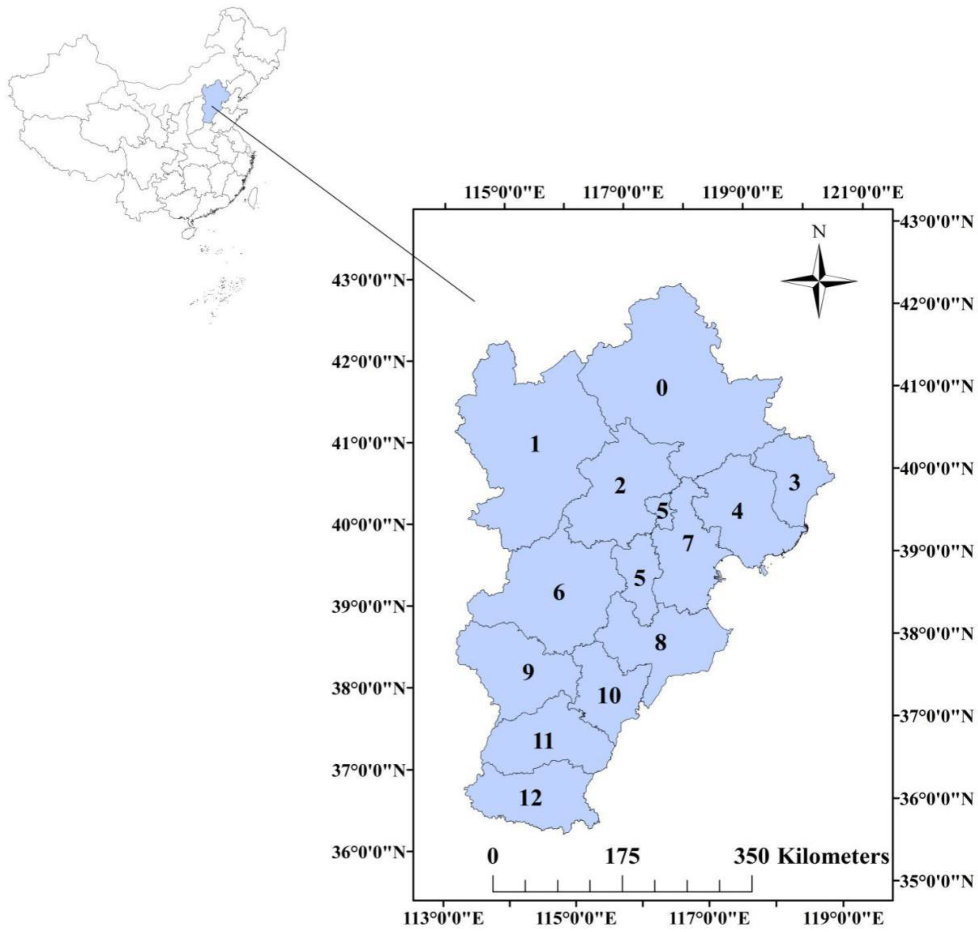
2.1. Study Area

The BTH region (36°01′ N–42°37′ N, 113°04′ E–119°53′ E, see Figure 1) is the capital economic circle in China. This region is situated in the North China Plain, connecting the Inner Mongolia Plateau in the north, the Loess Plateau in the west, and the Bohai Sea in the east. It is situated in a warm temperate zone with a semi-humid continental monsoon climate. The annual sunshine is 2500–2900 h, the annual total radiation is 5000–5800 MJ/mz, and the annual average temperature is 8–12.5 °C. Precipitation is mainly concentrated in summer, accounting for 60–75% of the entire year’s amount. The BTH is the most dynamic economic region in northern China. In 2019, the gross domestic product (GDP) of this region totaled 845.808 billion RMB, accounting for 8.5% of the country [35,36,37]. The development of the BTH region is a major national strategic issue.

2.2. Data Sources

We used both spatial and statistical data in this research. The spatial data comprised: (1) The digital elevation model (DEM) at a spatial resolution of 90 × 90 m, supplied by the Geo-spatial Data Cloud Station (http://www.giscloud.cn/) of the Computer Network Information Center of the Chinese Academy of Sciences. (2) Population and GDP data, rainfall data, and normalized vegetation index (NDVI) data at a spatial resolution of 1 × 1 km, supplied by the Resource and Environment Data Cloud Platform (http://www.resdc.cn/) of the Chinese Academy of Sciences. We used the inverse distance weighting method to interpolate the relevant missing data. (3) The net primary productivity (NPP) data at a spatial resolution of 1 × 1 km were provided by the MOD17A3 data set (https://lpdaac.usgs.gov/). (4) The land use and land cover change (LUCC) data at a spatial resolution of 300 × 300 m were provided by the European Space Agency (http://neo.ssa.esa.int/advanced-search) and were reclassified. The landscape was divided into eight categories: paddy fields, dry land, woodland, other woodland, shrub land, water areas, construction land, and barren land. (5) The soil data were provided by the World Soil Database (http://webarchive.iiasa.ac.at/Research/LUC/External-World-soil-database). The statistical data included grain production and other production supplies obtained from the Beijing Statistical Yearbook [38,39,40,41], Tianjin Statistical Yearbook [42,43,44,45], and Hebei Statistical Yearbook [46,47,48,49]. Population, GDP, and LUCC data were used to quantify urbanization levels. Other data were used to calculate ecosystem service values by empirical models.

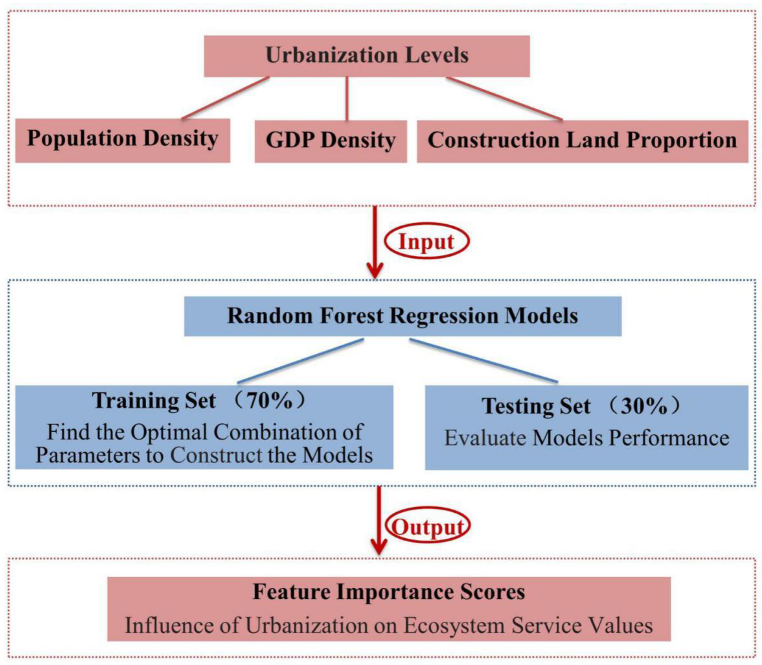
2.3. Selection of Urbanization Indicators

Urbanization is reflected in four aspects: Living standards improvement, population growth, economic development, and construction land expansion [50]. The improvements in the standard of living can be represented by population growth, economic development, and construction land expansion [27]. We described the urbanization levels of the BTH urban agglomeration in terms of population growth, economic development, and construction land expansion. The population density (person/km2) was made use of characterizing population urbanization, GDP density (yuan/km2) was made use of reflecting economic urbanization, and the construction land proportion in the every pixel (1 × 1 km) was made use of describing the situation of construction land expansion [22] (see Table 1).

2.4. RF Regression Model

RF is a machine learning method using a supervised learning algorithm that improves the stability and accuracy of regression and classification [30]. The RF method can reduce large bias and avoid over-fitting to a certain extent based on mean prediction of individual trees. RF is normally used to deal with regression and classification problems, and the methods of data treatment differ according to the details of the problem. In principle, an RF regression model can be designed by following the steps outlined below. When there is a training set D that contains N data points, we use RF to perform regression on the training set D. First, bootstrapping is used to select n subsets Di (the range of i is 1 to n) from the training set D as new training sets. Each of the Di contain N’ data points (the amount of data N’ in the subsets Di is the same as the amount N in the set D. However, the content is different, because elements in subsets Di can be repeated). Afterwards, using the regression algorithm on the n subsets Di, we have n results. Taking the average value of these results, we can obtain the final result of the RF regression model [51].
Based on the data for population, GDP, and LUCC, we generated raster maps of urbanization levels (population density, GDP density, and construction land proportion) at a spatial resolution of 1 × 1 km in 2000, 2005, 2010, and 2014. Then, we extracted relevant raster data as input to construct the RF regression model by Python. We randomly divided the data set into a training set (70% of the total) and a testing set (30% of the total). The training set was used for constructing the RF regression model under the optimal parameter combination, and the testing set was used for evaluating model performance. Finally, the RF regression model output importance scores for the three urbanization indicators (based on the Gini index) reflecting the extent of the effect of urbanization on ecosystem service in the BTH urban agglomeration in 2000–2014 (Figure 2).

2.5. Quantifying Ecosystem Services Using Empirical Models

Our study selected four kinds of ecosystem services (see Table 1), the methods of quantifying them are summarized as follows:
  • Food production
Food production is essential for sustainable development of the BTH region [52]. We calculated the annual amount of food production according to the method [22]. The calculation formula is as follows:
P x = i = 1 3 A × P ,
where Px (t/km2) is the annual amount of food production for grid x (1 km2). The subscript x refers to the grid point in the study area; i represents three types of food (grain, oil crops, and vegetables). A represents the area of cultivated land for grid point x. P refers to the average yield of the selected three food types per unit area [23,53], and the data were obtained from the Beijing Statistical Yearbook [38,39,40,41], Tianjin Statistical Yearbook [42,43,44,45], and Hebei Statistical Yearbook [46,47,48,49].
  • Carbon sequestration and oxygen production
We used the following equation to calculate the annual amounts of carbon sequestration and oxygen production [22,54].
C x = 1.63 × N P P x + 1.2 × N P P x ,
where Cx (t/km2) is the annual amount of carbon sequestration and oxygen production for grid x (1 km2); x refers to the grid point in the study area; and NPPx (t/km2) is the value of NPP for grid point x.
  • Water conservation
We calculated the annual amount of water conservation according to the method [55]. The calculation formula was as follows:
W x = P P T x E T x ,  
where Wx (mm) represents the amount of water conservation for grid point x (1 km2); x refers to the grid point in the study area; PPTx (mm) is the quantity of precipitation for grid point x; and ETx (mm) is the quantity of evapotranspiration for grid point x. ETx is calculated as
E T x   =   9.78   +   0.0072   ×   P E T × P P T x + 0.051   ×   L A I × P P T x ,
where PET (mm) represents potential evapotranspiration and can be obtained by a simple calculation method [56]. LAI is leaf area index, this can be obtained by using the relationship between NDVI and LAI under different land use types [57]. The coefficients of Equation (4) are defined through the calibration for the equation with statistically modeling of the relationships between observed data and estimated data by Jia et al. [55].
  • Soil conservation
We used the InVEST model to quantify soil conservation. The calculation formula of annual soil conservation function is as follows [27]:
S x   =   R K L S x   U S L E x   =   R x ×   K x   ×   L S x   ×   ( 1     C x ×   P x ) ,
where Sx (t/km2) represents the annual soil conservation function for grid point x (1 km2); x refers to the grid point in the study area. RKLSx (t/km2) is the annual amount of potential soil erosion for grid point x. USLEx (t/km2) is the annual amount of actual soil erosion for grid point x. Rx (MJ·mm/(km2·hr)) is the rainfall erosivity for grid point x, which can be calculated by the Brinell algorithm. Kx (t·km2·hr/(MJ·km2·mm)) is the soil erodibility factor for grid point x, which can be obtained by the estimation method for K in the EPIC model [58]. LSx is the slope length-gradient factor for grid point x. The InVEST model can automatically generate the result map according to the filled DEM. Cx and Px are the crop management factor and the governance measure factor for grid point x, respectively. The two factors for each land type were provided by Li et al. [59].

3. Results

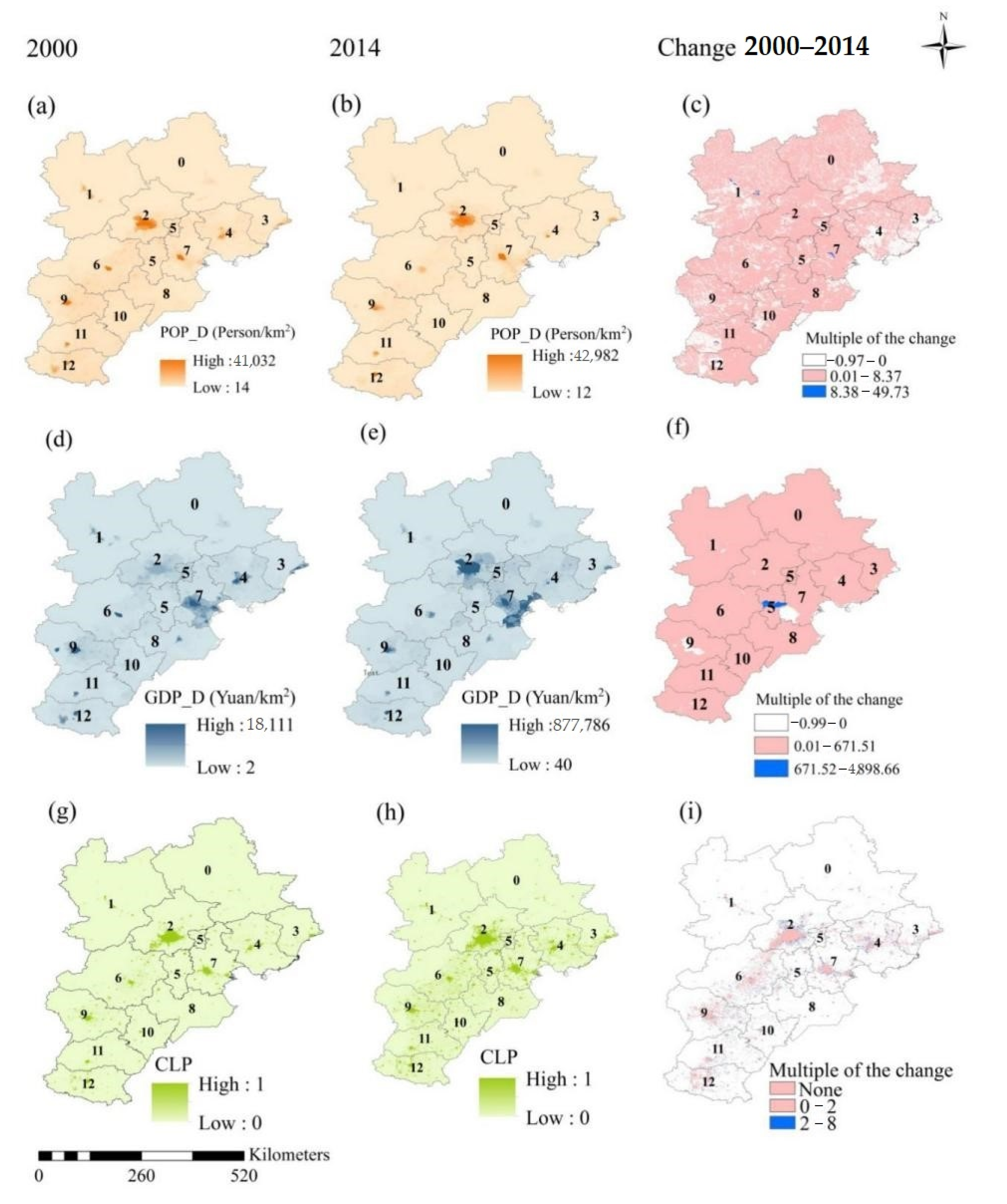
3.1. The Spatial and Temporal Patterns and Dynamic Characteristics of Urbanization Levels

The spatial and temporal patterns and dynamic characteristics of urbanization indicators of the BTH region in 2000 and 2014 are shown in Figure 3. The spatial patterns of POP_D (population density), GDP_D (gross domestic product density), and CLP (proportion of construction land) were generally consistent from 2000 to 2014. The higher levels of urbanization were mainly concentrated in two mega-cities, #2 (Beijing) and #7 (Tianjin) (Figure 3a,b,d,e,g,h). The temporal patterns of the three indicators were basically similar, with increasing averages in the entire BTH region. The population density was 343.61 person/km2 in 2000 and 443.62 person/km2 in 2014. The GDP density was 344.44 yuan/km2 in 2000 and 3130.86 yuan/km2 in 2014. The proportion of construction land was 0.03 in 2000 and 0.08 in 2014. They increased by 29.11%, 808.97%, and 166.67%, respectively. The growth of GDP density was much higher than the others (Table 2). As for dynamic characteristics of urbanization levels on the spatial and temporal scales, the population density increased in the wide range of the area (greater growth was mainly distributed in areas #1, 2, 7, and 11) and declined in a small part of the area. Similarly, the GDP density increased in the majority of the areas (greater growth was located in the area of #5) and declined in a few areas. The change in the proportion of construction land differed in that no changes occurred in most areas, and the increase was mainly distributed in areas #2, 4, 6, 7, 9, 11, and 12 (Figure 3c,f,i).

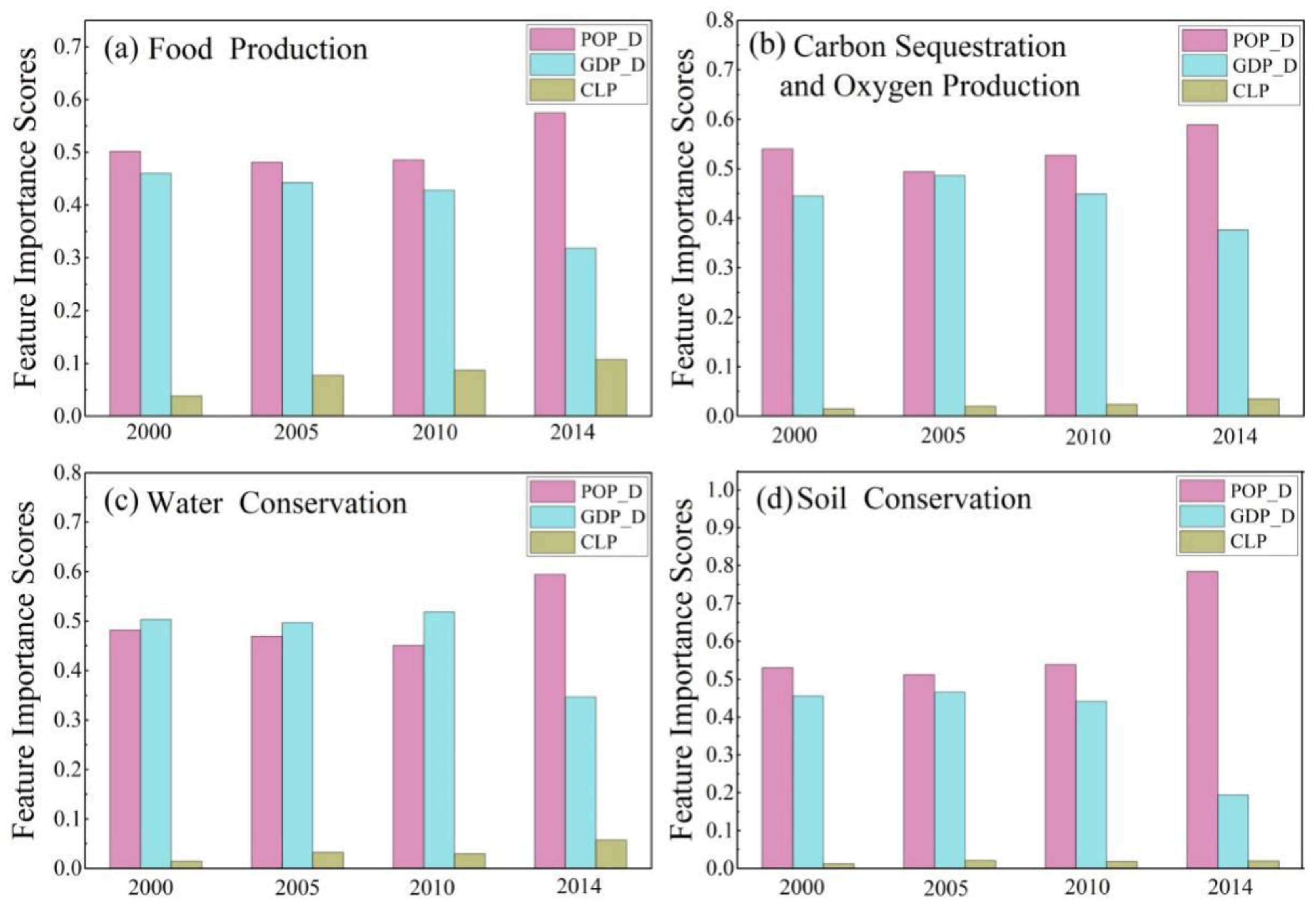
3.2. The Effect of Urbanization on Ecosystem Services in the BTH Urban Agglomeration

The feature importance scores from the RF regression model are shown in Figure 4. We measured the impacts of urbanization on ecosystem services in the BTH region in 2000–2014. For food production (ecosystem service indicator #1), the population density had the greatest impact followed by GDP density, and the proportion of construction land had the least impact (Figure 4a). The impact of urbanization on carbon sequestration and oxygen production (ecosystem service indicator #2) and soil conservation (ecosystem service indicator #4) were basically consistent (Figure 4b,d). In contrast, in 2000–2010, the GDP density had the greatest impact on water conservation (ecosystem service indicator #3) followed by population density, and the proportion of construction land had the least impact (Figure 4c). The changing trends of the effects of the three urbanization indicators were as follows: the effect of population density on food production had increased between 2000 and 2014 (the importance score of population density was 0.502 in 2000, while the score reached 0.575 in 2014); the effect of GDP density on food production had decreased from 2000 to 2014 (the importance score for GDP density was 0.460 in 2000 and 0.318 in 2014). The effect of construction land proportion on food production had also increased from 2000 to 2014 (the importance score for construction land proportion was 0.038 in 2000 and 0.107 in 2014) (Figure 4a). The trends of the effects of population density and GDP density on the other three ecosystem services were similar to those for food production (Figure 4b–d). The trends of the effect of construction land proportion on the other three ecosystem services were as follows: the effects of the proportion of construction land on carbon sequestration and oxygen production, and water conservation increased from 2000 to 2014 (Figure 4b,c), while the effect on soil conservation was relatively stable in 2000–2014 (the importance scores of construction land proportion were 0.013 in 2000 and 0.020 in 2014) (Figure 4d).

3.3. The Comparisons of Simulations between the RF Regression Model and an Empirical Model

We used both empirical models and the RF regression model to estimate the values of the ecosystem services (ecosystem service values estimated by empirical models could see Figure S1). The results of comparisons between the RF regression model and the empirical models using the testing set for 2000 were plotted with standard deviation bars (Figure 5). The R2 values for the four kinds of ecosystem services ranged from 0.714 to 0.986 (p < 0.05 for each). The highest R2 values were found for carbon sequestration and oxygen production, followed by food production and water conservation. The R2 values for those services were all greater than 0.9 (Figure 5a–c). The lowest R2 was found for soil conservation (R2 = 0.714) (Figure 5d).

4. Discussions

4.1. The Spatio-Temporal Dynamic Characteristics of Urbanization

The average values of population density, GDP density, and the proportion of construction land in the BTH region from 2000 to 2014 are shown in Table 2. The increase rates for population density, GDP density, and construction land proportion were 29.11%, 808.97%, and 166.67%, respectively. The population density and GDP density increased in a wide range of areas and declined in a small part of the region in 2000–2014 (Figure 3c,f). The situation for construction land proportion was different. In the majority of areas, this was unchanged, the increase has been mainly distributed in small areas (Figure 3i). These results demonstrated that the urbanization of the BTH has surpassed the initial stage represented by population concentration and land expansion and has entered the middle stage represented by population concentration and economic growth [61].
The economy emerged as an explosive growth accompanied by the expansion of urban areas. Our study has highlighted two key factors causing this phenomenon: (1) National policy, (2) China’s admission to the World Trade Organization (WTO) in 2001 under the background of economic globalization [62]. This has a profound impact on China’s urbanization. At the country level, the rate of urbanization rose from 17.9% in 1978 to 54.8% in 2014 [63]. The transformations of urbanization are described as both high-speed and great using conventional indicators of growth (population, GDP, urban area) [64]. However, the population of the BTH has shown a relatively small growth trend, as China implemented a one-child family policy to relieve the pressure of a massive population increase since 1982 [65]. Facing these changes, some debates have emerged to assess the forces driving the urbanization of China. Several important forces have been deeply discussed [66], e.g., economic globalization [67], national policy [68], inter-regional competition [69], and spatial administrative reorganization [70]. Currently, the BTH urban agglomeration is still growing. Geographically predicting the policy influences on urban development remains a big challenge.

4.2. The Quantification of the Effect of Urbanization on Ecosystem Services in the BTH Urban Agglomeration Using the RF Regression Model

Differing from traditional methods, our study confirmed that RF regression models could directly reveal the effect of urbanization on ecosystem services based on the importance scores of three urbanization indicators. Based on our results, the importance scores for population density and GDP density were much higher than for construction land proportion regarding the four ecosystem services (Figure 4). This suggested that population density and GDP density were the key factors affecting ecosystem services, and the proportion of construction land had a lesser impact. In general, the expansion of the urban population and rapid economic development were the dominant factors affecting ecosystem services. In particular, the accumulation of industry and population growth had greatly increased the consumption of land resources, water resources, and other energy sources. These use patterns had caused significant levels of pollution that negatively affected the ecosystem [71]. We found changing trends in the effect of urbanization on ecosystem services: the effect of population density increased, while the effect of construction land proportion was consistent with population density. In contrast, the effect of GDP density decreased (Figure 4). These results indicated that controlling the population and GDP levels is important for the sustainable development of cities in large urban areas.

4.3. The Comparisons of Simulations between RF Regression and Empirical Models

The results of comparisons between the RF regression model and empirical models for assessing ecosystem services using the testing set in 2000 are shown in Figure 5. The R2 values for four kinds of ecosystem service indicators were all more than 0.9 (Figure 5a–c). In terms of the simulation outputs, both RF regression and empirical models were able to effectively simulate ecosystem service indicators. There was a slight difference between the RF regression model and empirical models. The R2 for soil conservation was only 0.714. The simulated result of the RF regression model was lower than for the empirical model in the high value for soil conservation (Figure 5d). This implied that the soil conservation was differently estimated by the RF regression and empirical models. This might result in a difficulty to assess the effect of the urbanization on soil conservation. Nevertheless, it may not be a significant issue in the BTH region, as this area primarily contains fertile farmland in the second largest flatland of China. There might not be a significant correlation between urbanization and soil conservation [72].

4.4. Uncertainties

In mapping urbanization levels using remote sensing (RS) data, there were differences in the urbanization levels under different sources of data. We used the LUCC data to calculate the proportion of construction land, and the data of LUCC were provided by the European Space Agency (http://neo.ssa.esa.int/advanced-search). It is possible that the spatio-temporal patterns of construction land proportion would not be completely consistent if the LUCC data were obtained from other RS data. To compare the results employing different methods, four empirical models were chosen for testing the performance. Although both RF regression and empirical models demonstrated consistently reasonable estimates in most of the simulation outputs, there was still some discrepancy in soil conservation. Currently, it is still a challenge to obtain observed ecosystem service values. Future improvement in the observation of ecosystems services and model integration with these observations could certainly reduce the uncertainties in our study.

5. Conclusions

The rapid economic development at national scale involves many aspects, in which some major sections may have negative effects on ecosystem services. Especially, the population growth, construction land expansion, and traffic management present serious challenges to the sustainable development of the urban agglomeration. As the largest urbanization in China, BTH urban agglomeration has the most representative features. Through exploring the spatial and temporal dynamic characteristics of urbanization levels from 2000 to 2014 in the BTH using spatial data analysis, we found that the urbanization of the BTH was at a stage represented by population concentration and economic growth. The results suggested that population density and GDP density were the two dominant factors affecting ecosystem services, and that construction land proportion had a lesser impact on ecosystem services. Our study using the RF regression model demonstrated the changing trends of the effect of urbanization on ecosystem services. The effect of population density on ecosystem services increased, and the effect of the proportion of construction land on ecosystem services was consistent with population density. In contrast, the effect of GDP density on ecosystem services decreased. This study paves the way for quantitative evaluation of the effect of urbanization on ecosystem services at a regional scale.

Supplementary Materials

The following are available online at https://www.mdpi.com/2071-1050/12/24/10233/s1, Figure S1: Spatial and temporal patterns and dynamic characteristics of ecosystem service values from empirical models for the Beijing, Tianjin, and Hebei (BTH) region in 2000–2014.

Author Contributions

Conceptualization, S.L., M.Y., and Y.M. (Yuling Mou), Y.M. (Yanrong Meng); methodology, S.L. and X.Z.; Writing—Original Draft, S.L.; Writing—Review & Editing, C.P. and X.Z. All authors have read and agreed to the published version of the manuscript.

Funding

This research was funded by the National Key R&D Program of China [2016YFC0500203] and the Natural Sciences and Engineering Research Council of Canada (NSERC) Discover Grant.

Acknowledgments

This work was supported by the National Key R&D Program of China [2016YFC0500203] and the Natural Sciences and Engineering Research Council of Canada (NSERC) Discover Grant. We thank Hanwei Li and Hanxiong Song for the data collection and processing.

Conflicts of Interest

The authors declare no conflict of interest.

References

  1. Su, S.; Jiang, Z.; Zhang, Q.; Zhang, Y. Transformation of agricultural landscapes under rapid urbanization: A threat to sustainability in Hang-Jia-Hu region, China. Appl. Geogr. 2011, 31, 439–449. [Google Scholar] [CrossRef]
  2. De Groot, R.; Brander, L.; van der Ploeg, S.; Costanza, R.; Bernard, F.; Braat, L.; Christie, M.; Crossman, N.; Ghermandi, A.; Hein, L.; et al. Global estimates of the value of ecosystems and their services in monetary units. Ecosyst. Serv. 2012, 1, 50–61. [Google Scholar] [CrossRef]
  3. Wang, Y.; Gao, J.; Wang, J.; Qiu, J. Value assessment of ecosystem services in nature reserves in Ningxia, China: A response to ecological restoration. PLoS ONE 2014, 9, e89174. [Google Scholar] [CrossRef]
  4. Chen, Q.; Mei, K.; Dahlgren, R.A.; Wang, T.; Gong, J.; Zhang, M. Impacts of land use and population density on seasonal surface water quality using a modified geographically weighted regression. Sci. Total Environ. 2016, 572, 450–466. [Google Scholar] [CrossRef] [Green Version]
  5. Holt, A.R.; Mears, M.; Maltby, L.; Warren, P. Understanding spatial patterns in the production of multiple urban ecosystem services. Ecosyst. Serv. 2015, 16, 33–46. [Google Scholar] [CrossRef] [Green Version]
  6. Mach, M.E.; Martone, R.G.; Chan, K.M.A. Human impacts and ecosystem services: Insufficient research for trade-off evaluation. Ecosyst. Serv. 2015, 16, 112–120. [Google Scholar] [CrossRef]
  7. Xue, M.; Luo, Y. Dynamic variations in ecosystem service value and sustainability of urban system: A case study for Tianjin city, China. Cities 2015, 46, 85–93. [Google Scholar] [CrossRef]
  8. Pardo, M.D.C.; Martínez, P.F.; Martínez, J.M.G.; Martín, J.M.M. Modelling natural capital: A proposal for a mixed multi-criteria approach to assign management priorities to ecosystem. Contemp. Econ. 2020, 14, 22–38. [Google Scholar] [CrossRef]
  9. Bateman, I.J.; Jones, A.P. Contrasting conventional with multi-level modeling approaches to meta-analysis: Expectation consistency in U.K. woodland recreation values. Land Econ. 2003, 79, 235–258. [Google Scholar] [CrossRef]
  10. Rosado, M.A.; Cunha-E-Sá, M.A.; Ducla-Soares, M.M.; Nunes, L.C. Combining averting behavior and contingent valuation data: An application to drinking water treatment in Brazil. Environ. Dev. Econ. 2006, 11, 729–746. [Google Scholar] [CrossRef]
  11. Chen, W.Y.; Hua, J. Heterogeneity in resident perceptions of a bio-cultural heritage in Hong Kong: A latent class factor analysis. Ecosyst. Serv. 2017, 24, 170–179. [Google Scholar] [CrossRef]
  12. Barbier, E.B. Valuing ecosystem services as productive inputs. Econ. Policy 2007, 22, 178–229. [Google Scholar] [CrossRef]
  13. Li, P.; Zhou, G.; Du, H.; Lu, D.; Mo, L.; Xu, X.; Shi, Y.; Zhou, Y. Current and potential carbon stocks in Moso bamboo forests in China. J. Environ. Manag. 2015, 156, 89–96. [Google Scholar] [CrossRef] [PubMed]
  14. Wang, W.; Guo, H.; Chuai, X.; Dai, C.; Lai, L.; Zhang, M. The impact of land use change on the temporospatial variations of ecosystems services value in China and an optimized land use solution. Environ. Sci. Policy 2014, 44, 62–72. [Google Scholar] [CrossRef]
  15. Song, X.Z.; Zhao, C.X.; Wang, X.L.; Li, J. Study of nitrate leaching and nitrogen fate under intensive vegetable production pattern in northern China. Comptes Rendus Biol. 2009, 332, 385–392. [Google Scholar] [CrossRef]
  16. Shoyama, K.; Kamiyama, C.; Morimoto, J.; Ooba, M.; Okuro, T. A review of modeling approaches for ecosystem services assessment in the Asian region. Ecosyst. Serv. 2017, 26, 316–328. [Google Scholar] [CrossRef]
  17. Crossman, N.D.; Burkhard, B.; Nedkov, S. Quantifying and mapping ecosystem services. Int. J. Biodivers. Sci. Ecosyst. Serv. Manag. 2012, 8, 1–4. [Google Scholar] [CrossRef]
  18. Goldstein, J.H.; Caldarone, G.; Duarte, T.K.; Ennaanay, D.; Hannahs, N.; Mendoza, G.; Polasky, S.; Wolny, S.; Daily, G.C. Integrating ecosystem-service tradeoffs into land-use decisions. Proc. Natl. Acad. Sci. USA 2012, 109, 7565–7570. [Google Scholar] [CrossRef] [Green Version]
  19. Burkhard, B.; Crossman, N.; Nedkov, S.; Petz, K.; Alkemade, R. Mapping and modelling ecosystem services for science, policy and practice. Ecosyst. Serv. 2013, 4, 1–3. [Google Scholar] [CrossRef]
  20. Costanza, R.; de Groot, R.; Sutton, P.; van der Ploeg, S.; Anderson, S.J.; Kubiszewski, I.; Farber, S.; Turner, R.K. Changes in the global value of ecosystem services. Glob. Environ. Chang. 2014, 26, 152–158. [Google Scholar] [CrossRef]
  21. Kindu, M.; Schneider, T.; Teketay, D.; Knoke, T. Changes of ecosystem service values in response to land use/land cover dynamics in Munessa-Shashemene landscape of the Ethiopian highlands. Sci. Total Environ. 2016, 547, 137–147. [Google Scholar] [CrossRef]
  22. Wang, J.; Zhou, W.; Pickett, S.T.A.; Yu, W.; Li, W. A multiscale analysis of urbanization effects on ecosystem services supply in an urban megaregion. Sci. Total Environ. 2019, 662, 824–833. [Google Scholar] [CrossRef]
  23. Zhang, D.; Huang, Q.; He, C.; Wu, J. Impacts of urban expansion on ecosystem services in the Beijing-Tianjin-Hebei urban agglomeration, China: A scenario analysis based on the Shared Socioeconomic Pathways. Resour. Conserv. Recycl. 2017, 125, 115–130. [Google Scholar] [CrossRef]
  24. Faulkner, S. Urbanization impacts on the structure and function of forested wetlands. Urban Ecosyst. 2004, 7, 89–106. [Google Scholar] [CrossRef]
  25. Su, S.; Li, D.; Hu, Y.; Xiao, R.; Zhang, Y. Spatially non-stationary response of ecosystem service value changes to urbanization in Shanghai, China. Ecol. Indic. 2014, 45, 332–339. [Google Scholar] [CrossRef]
  26. Zhang, W.; Yang, D.; Huo, J. Studies of the relationship between city size and urban benefits in China based on a panel data model. Sustainability 2016, 8, 554. [Google Scholar] [CrossRef] [Green Version]
  27. Peng, J.; Tian, L.; Liu, Y.; Zhao, M.; Hu, Y.; Wu, J. Ecosystem services response to urbanization in metropolitan areas: Thresholds identification. Sci. Total Environ. 2017, 607–608, 706–714. [Google Scholar] [CrossRef]
  28. Sun, X.; Crittenden, J.C.; Li, F.; Lu, Z.; Dou, X. Urban expansion simulation and the spatio-temporal changes of ecosystem services, a case study in Atlanta Metropolitan area, USA. Sci. Total Environ. 2018, 622–623, 974–987. [Google Scholar] [CrossRef]
  29. Wu, M.; Ren, X.; Che, Y.; Yang, K. A Coupled SD and CLUE-S Model for Exploring the Impact of Land Use Change on Ecosystem Service Value: A Case Study in Baoshan District, Shanghai, China. Environ. Manag. 2015, 56, 402–419. [Google Scholar] [CrossRef]
  30. Breiman, L. Random forests. Mach. Learn. 2001, 45, 5–32. [Google Scholar] [CrossRef] [Green Version]
  31. Svetnik, V.; Liaw, A.; Tong, C.; Christopher Culberson, J.; Sheridan, R.P.; Feuston, B.P. Random Forest: A Classification and Regression Tool for Compound Classification and QSAR Modeling. J. Chem. Inf. Comput. Sci. 2003, 43, 1947–1958. [Google Scholar] [CrossRef]
  32. Hu, X.; Hong, W.; Qiu, R.; Hong, T.; Chen, C.; Wu, C. Geographic variations of ecosystem service intensity in Fuzhou City, China. Sci. Total Environ. 2015, 512–513, 215–226. [Google Scholar] [CrossRef]
  33. Wan, L.; Ye, X.; Lee, J.; Lu, X.; Zheng, L.; Wu, K. Effects of urbanization on ecosystem service values in a mineral resource-based city. Habitat Int. 2015, 46, 54–63. [Google Scholar] [CrossRef]
  34. Wu, K.Y.; Ye, X.Y.; Qi, Z.F.; Zhang, H. Impacts of land use/land cover change and socioeconomic development on regional ecosystem services: The case of fast-growing Hangzhou metropolitan area, China. Cities 2013, 31, 276–284. [Google Scholar] [CrossRef]
  35. Beijing Municipal Bureau of Statistics. Beijing Statistical Yearbook; China Statistics Press (CSP) Publishing: Beijing, China, 2020. [Google Scholar]
  36. Tianjin Municipal Bureau of Statistics. Tianjin Statistical Yearbook; China Statistics Press (CSP) Publishing: Beijing, China, 2020. [Google Scholar]
  37. Hebei Municipal Bureau of Statistics. Hebei Statistical Yearbook; China Statistics Press (CSP) Publishing: Beijing, China, 2020. [Google Scholar]
  38. Beijing Municipal Bureau of Statistics. Beijing Statistical Yearbook; China Statistics Press (CSP) Publishing: Beijing, China, 2001. [Google Scholar]
  39. Beijing Municipal Bureau of Statistics. Beijing Statistical Yearbook; China Statistics Press (CSP) Publishing: Beijing, China, 2006. [Google Scholar]
  40. Beijing Municipal Bureau of Statistics. Beijing Statistical Yearbook; China Statistics Press (CSP) Publishing: Beijing, China, 2011. [Google Scholar]
  41. Beijing Municipal Bureau of Statistics. Beijing Statistical Yearbook; China Statistics Press (CSP) Publishing: Beijing, China, 2015. [Google Scholar]
  42. Tianjin Municipal Bureau of Statistics. Tianjin Statistical Yearbook; China Statistics Press (CSP) Publishing: Beijing, China, 2001. [Google Scholar]
  43. Tianjin Municipal Bureau of Statistics. Tianjin Statistical Yearbook; China Statistics Press (CSP) Publishing: Beijing, China, 2006. [Google Scholar]
  44. Tianjin Municipal Bureau of Statistics. Tianjin Statistical Yearbook; China Statistics Press (CSP) Publishing: Beijing, China, 2011. [Google Scholar]
  45. Tianjin Municipal Bureau of Statistics. Tianjin Statistical Yearbook; China Statistics Press (CSP) Publishing: Beijing, China, 2015. [Google Scholar]
  46. Hebei Municipal Bureau of Statistics. Hebei Statistical Yearbook; China Statistics Press (CSP) Publishing: Beijing, China, 2001. [Google Scholar]
  47. Hebei Municipal Bureau of Statistics. Hebei Statistical Yearbook; China Statistics Press (CSP) Publishing: Beijing, China, 2006. [Google Scholar]
  48. Hebei Municipal Bureau of Statistics. Hebei Statistical Yearbook; China Statistics Press (CSP) Publishing: Beijing, China, 2011. [Google Scholar]
  49. Hebei Municipal Bureau of Statistics. Hebei Statistical Yearbook; China Statistics Press (CSP) Publishing: Beijing, China, 2015. [Google Scholar]
  50. Bai, X.; Shi, P.; Liu, Y. Realizing China’s urban dream. Nature 2014, 509, 158–160. [Google Scholar] [CrossRef] [Green Version]
  51. Fernandez-Gonzalez, P.; Bielza, C.; Larranaga, P. Random Forests for Regression as a Weighted Sum of k-Potential Nearest Neighbors. IEEE Access 2019, 7, 25660–25672. [Google Scholar] [CrossRef]
  52. Li, B.; Chen, D.; Wu, S.; Zhou, S.; Wang, T.; Chen, H. Spatio-temporal assessment of urbanization impacts on ecosystem services: Case study of Nanjing City, China. Ecol. Indic. 2016, 71, 416–427. [Google Scholar] [CrossRef]
  53. Xie, W.; Huang, Q.; He, C.; Zhao, X. Projecting the impacts of urban expansion on simultaneous losses of ecosystem services: A case study in Beijing, China. Ecol. Indic. 2018, 84, 183–193. [Google Scholar] [CrossRef]
  54. Li, J.; Zhou, Z.X. Natural and human impacts on ecosystem services in Guanzhong—Tianshui economic region of China. Environ. Sci. Pollut. Res. 2016, 23, 6803–6815. [Google Scholar] [CrossRef]
  55. Jia, X.; Fu, B.; Feng, X.; Hou, G.; Liu, Y.; Wang, X. The tradeoff and synergy between ecosystem services in the Grain-for-Green areas in Northern Shaanxi, China. Ecol. Indic. 2014, 43, 103–113. [Google Scholar] [CrossRef]
  56. Hamon, W.R. Computation of direct runoff amounts from storm rainfall. Int. Assoc. Sci. Hydrol. Publ. 1963, 63, 52–62. [Google Scholar]
  57. Sun, P.; Liu, S.; Liu, J.; Li, C.; Lin, Y.; Jiang, H. Derivation and validation of leaf area index maps using NDVI data of different resolution satellite imageries. Acta. Ecol. Sin. 2006, 26, 3826–3834. (In Chinese) [Google Scholar]
  58. Sharpley, A.N.; Williams, J.R. EPIC: The Erosion-Productivity Impact Calculator, 1.0 Model Documentation; Technical Bulletin; United States Department of Agriculture: Washington, DC, USA, 1990.
  59. Li, X.S.; Ji, C.C.; Zeng, Y.; Yan, N.N.; Wu, B.F. Dynamics of water and soil loss based on remote sensing and GIS: A case study in Chicheng County of Hebei Province. Chin. J. Ecol. 2009, 28, 1723–1729. (In Chinese) [Google Scholar]
  60. Costanza, R.; D’Arge, R.; De Groot, R.; Farber, S.; Grasso, M.; Hannon, B.; Limburg, K.; Naeem, S.; O’Neill, R.V.; Paruelo, J.; et al. The value of the world’s ecosystem services and natural capital. Nature 1997, 387, 253–260. [Google Scholar] [CrossRef]
  61. Zhou, D.; Tian, Y.; Jiang, G. Spatio-temporal investigation of the interactive relationship between urbanization and ecosystem services: Case study of the Jingjinji urban agglomeration, China. Ecol. Indic. 2018, 95, 152–164. [Google Scholar] [CrossRef]
  62. The Central People’s Government of the People’s Republic of China. China and the World Trade Organization; CPG Publishing: Beijing, China, 2018. [Google Scholar]
  63. Shi, C.; Tang, B.S. Institutional change and diversity in the transfer of land development rights in China: The case of Chengdu. Urban Stud. 2020, 57, 473–489. [Google Scholar] [CrossRef]
  64. Chien, S.-S.; Woodworth, M.D. China’s Urban Speed Machine: The Politics of Speed and Time in a Period of Rapid Urban Growth. Int. J. Urban Reg. Res. 2018, 42, 723–737. [Google Scholar] [CrossRef]
  65. The National People’s Congress of the People’s Republic of China. Constitution of the People’s Republic of China; NPC Publishing: Beijing, China, 1982. [Google Scholar]
  66. Ma, L.J.C. Urban administrative restructuring, changing scale relations and local economic development in China. Polit. Geogr. 2005, 24, 477–497. [Google Scholar] [CrossRef]
  67. Zhang, J.; Wu, F. China’s changing economic governance: Administrative annexation and the reorganization of local governments in the Yangtze River Delta. Reg. Stud. 2006, 40, 3–21. [Google Scholar] [CrossRef]
  68. Chien, S.S. Institutional innovations, asymmetric decentralization, and local economic development: A case study of Kunshan, in post-Mao China. Environ. Plan. C Gov. Policy 2007, 25, 269–290. [Google Scholar] [CrossRef]
  69. Wu, F.; Zhang, J. Planning the competitive city-region: The emergence of strategic development plan in China. Urban Aff. Rev. 2007, 42, 714–740. [Google Scholar] [CrossRef]
  70. Lin, G.C.S.; Ho, S.P.S. The state, land system, and land development processes in contemporary China. Ann. Assoc. Am. Geogr. 2005, 95, 411–436. [Google Scholar] [CrossRef]
  71. Huang, M.; Yang, F.; Zheng, S. Impact of urbanization process on ecosystem service value in China. Res. Soil. Water. Conserv. 2019, 26, 352–359. (In Chinese) [Google Scholar]
  72. Zhang, W. The coupling relationship between the ecosystem service value of farmland and urbanization in Guanzhong-Tianshui Economic Zone. Master’s Thesis, Shaanxi Normal University, Xian, Shaanxi, June 2015. [Google Scholar]
Figure 1. Location of the Beijing-Tianjin-Hebei (BTH) urban agglomeration. The numbers in maps represent each district (0, Chengde; 1, Zhangjiakou; 2, Beijing; 3, Qinhuangdao; 4, Tangshan; 5, Langfang; 6, Baoding; 7, Tianjin; 8, Cangzhou; 9, Shijiazhuang; 10, Hengshui; 11, Xingtai; 12, Handan).
Sustainability 12 10233 g001
Figure 2. Flow diagram of the random forest (RF) regression model. GDP: Gross Domestic Product. Feature Importance Scores represent the importance scores of three urbanization levels. The grid data (210,000) were extracted from raster maps of population density, GDP density, and the proportion of construction land as input to construct the RF regression model by Python. The model outputs feature importance scores (the Gini index can be used to measure the contribution of each feature in the RF regression model; the contributions of features represent importance scores). The scores reflect the effect of urbanization on ecosystem service values.
Sustainability 12 10233 g002
Figure 3. Spatial and temporal patterns and dynamic characteristics of urbanization levels of the Beijing, Tianjin, and Hebei (BTH) region in 2000–2014. POP_D is population density. GDP_D denotes gross domestic product (GDP) density, and CLP represents construction land proportion. The Yuan is the basic unit of Chinese currency. The numbers in the maps represent each district (0, Chengde; 1, Zhangjiakou; 2, Beijing; 3, Qinhuangdao; 4, Tangshan; 5, Langfang; 6, Baoding; 7, Tianjin; 8, Cangzhou; 9, Shijiazhuang; 10, Hengshui; 11, Xingtai; 12, Handan). (a,b) denote spatial and temporal patterns of POP_D in 2000 and 2014, respectively; (c) denotes dynamic changes of POP_D from 2000 to 2014. (d,e) denote spatial and temporal patterns of GDP_D in 2000 and 2014, respectively; (f) denotes dynamic changes of GDP_D from 2000 to 2014. (g,h) denote spatial and temporal patterns of CLP in 2000 and 2014, respectively; (i) denotes dynamic changes of CLP from 2000 to 2014.
Sustainability 12 10233 g003
Figure 4. The feature importance scores from the random forest (RF) regression model in the Beijing, Tianjin, and Hebei (BTH) region in 2000–2014. POP_D is population density, GDP_D denotes gross domestic product (GDP) density, and CLP represents construction land proportion. Feature Importance Scores represent the importance scores for the three urbanization measures. (ad) represent the importance scores for the three urbanization measures (POP_D, GDP_D, CLP) on food production, carbon sequestration and oxygen production, water conservation, and soil conservation in the BTH region in 2000–2014, respectively.
Sustainability 12 10233 g004
Figure 5. The comparisons between the simulations using the random forest (RF) regression model and empirical models based on the data of the testing set. Empirical model (a) refers to formula (1). Empirical model (b) refers to formula (2). Empirical model (c) refers to formula (3). Empirical model (d) refers to formula (5). The black dots represent the averages of simulations of the model, and the sizes of the dots represent the amount of grid data. Food production from the empirical model in (a) does not have a standard deviation, as the data for the average yield of the selected grain, oil crops, and vegetables per unit area were gathered according to administrative region.
Sustainability 12 10233 g005
Table 1. The description of urbanization indicators and ecosystem service indicators.
IndicatorsProperty and Role
Urbanization POP_D (person/km2)Reflect population urbanization
GDP_D (yuan/km2)Reflect economic urbanization
CLPReflect the situation of construction land expansion
Ecosystem
Service
Food Production (t/km2)Provisioning service of ecosystem service function
Carbon Sequestration and Oxygen Production (t/km2)Regulating service of ecosystem service function
Water Conservation (mm)Provisioning service of ecosystem service function
Soil Conservation (t/km2)Supporting service of ecosystem service function
Notes: (1) POP_D: population density. GDP_D: gross domestic product (GDP) density. CLP: construction land proportion. (2) The Yuan is the basic unit of Chinese currency. (3) The types of ecosystem services are based on the classification system proposed by Costanza et al. [60].
Table 2. Changes in urbanization levels of the entire Beijing, Tianjin, and Hebei (BTH) region in 2000–2014.
Levels20002005201020142000–2014 (%)
POP_D (person/km2)343.61376.20427.21443.6229.11
GDP_D (yuan/km2)344.44728.821306.843130.86808.97
CLP0.030.050.060.08166.67
Notes: (1) POP_D: population density. GDP_D: gross domestic product (GDP) density. CLP: construction land proportion. (2) The Yuan is the basic unit of Chinese currency.
Publisher’s Note: MDPI stays neutral with regard to jurisdictional claims in published maps and institutional affiliations.

