Article

Life Cycle Assessment of Biogas Production from Unused Grassland Biomass Pretreated by Steam Explosion Using a System Expansion Method

1
Institute of Agricultural Engineering, University of Natural Resources and Life Sciences Vienna, Peter Jordan Str. 82, 1190 Vienna, Austria
2
Fachhochschule Burgenland GmbH, Steinamangerstr. 21, 7423 Pinkafeld, Austria
3
City of Fort Collins, 222 Laporte Ave, Fort Collins, CO 80521, USA
*
Author to whom correspondence should be addressed.
Sustainability 2020, 12(23), 9945; https://doi.org/10.3390/su12239945
Submission received: 21 October 2020 / Revised: 18 November 2020 / Accepted: 23 November 2020 / Published: 27 November 2020

Abstract

:
Reforestation is a threat to permanent grasslands in many alpine regions. Using these areas to produce biogas energy may help to preserve these important landscapes and save fossil fuels by adding a renewable local heat and electricity source. This case study compares (a) a status quo (SQ) reference scenario with heating oil, wood-chips, and grid electricity as municipal energy sources, and (b) a hypothetical local biogas (LB) scenario (to also be used as a municipal energy source) based on a 500-kWel biogas plant with steam explosion pretreatment. Here, hay from previously unused grassland is the main biogas substrate, whereas, in the reference SQ scenario, these grasslands remain unused. Life cycle assessment (LCA) results for LB and SQ scenarios are significantly different at p < 0.05 in all six impact categories. In three categories, the LB scenario has lower impacts than the SQ scenario, including climate change (0.367 CO2-eq kWhel-1 versus 0.501 CO2-eq kWhel-1). Dominant contributions to climate change in the SQ scenario are from the extant municipal energy sources that the LB biogas plant would replace; in the LB scenario, important contributions include unburned methane from the biogas plant, as well as CO2 emissions from hay production machines. In summary, important environmental impacts can be reduced and alpine grasslands can be preserved by biogas production from that grass. The advantages of integrating a local biogas plant in municipal energy and waste systems depend strongly on the extant municipal energy system characteristics.

1. Introduction

Grasslands have a wide range of ecological functions and are home to highly diverse, specialized ecosystems. For alpine communities, they also play a significant role in winter and summer tourism, upon which these communities are economically dependent. A growing portion of alpine grasslands in Austria is no longer used for extensive forage production, due to difficult farming conditions, competition with intensive livestock operations, and the lack of a new generation of farmers [1]. Where forage production has ceased, using the grass to generate renewable electricity and heat from biogas could save fossil fuels and contribute to covering the energy demand generated by the tourism industry. In addition, local organic residues that are partly generated by tourism could be used as supplemental biogas substrates, increasing energy output and forming an integrated agromunicipal resource system [2].
Biogas generation from lignified biomass, such as late-cut grass from abandoned alpine grassland, generally requires pretreatment to increase digestibility. Steam explosion pretreatment (SEP) has been shown to improve the digestibility of lignified biomass such as agricultural residues and late-harvested grass with low feed quality [3,4,5,6,7]. Briefly, the SEP process exposes biomass to steam at a temperature up to 160–220 °C and under high pressure for varying retention periods [3]. Then, the biomass–steam mixture is abruptly depressurized, resulting in thermochemical and mechanical decomposition of the biomass. SEP not only increases the decomposition rate of the biomass but also increases specific biogas yields. It is considered environmentally advantageous as it boosts energy efficiency [8] and does not require the use of chemical additives or catalysts. SEP has also been shown to have an odor-reducing and sanitizing effect on organic wastes [8,9]. Digestate can thus be applied directly to fields without further treatment, facilitating closed nutrient cycles [10]. Implementing SEP has been shown to make the entire process of biogas production more economical [11].
The environmental impacts of biomass utilization strategies should be carefully assessed. Life cycle assessment (LCA) is an established, comprehensive approach to quantifying the environmental impacts of products and services [12], as well as entire technical systems. LCA literature on the effect of SEP on biogas production is sparse and even more so when it comes to the assessment of biogas production from extensively or formerly unused grasslands. Bedoić et al. [13] dealt with “residue grass” as input in biogas production but not from extensive alpine areas in Austria and without SEP. They concluded that they see some potential in the future use of grass in the production of biogas energy. Vo et al. [14] assessed the influence on sustainability and carbon intensity of grass as input substrate for biogas production but not for lignified substrates and therefore without pretreatment. Wang et al. [15] conducted an LCA for five different pretreatment combinations, including SEP, on biofuel generation from wheat straw. SEP with a catalyst was found to be environmentally favorable in comparison to the other pretreatment technologies. Prasad et al. [16] compared the environmental impacts of SEP to three other pretreatment technologies on a laboratory scale for lignocellulosic biomass. They found SEP to have the second lowest impacts for two of the four impact categories studied, and the third lowest for the other two categories. Schumacher et al. [17] compared the energy balance of biogas from maize silage and whole-plant triticale with and without SEP. They concluded that the energy demand for the pretreatment makes SEP an unfavorable option. On the other hand, Kral et al. [2] found that biogas production from maize stover with SEP had far lower impacts than conventional biogas production from maize silage. A recent literature review on LCA papers dealing with agro-biogas systems [18] did not show any results of energy systems comparable to the case studies of the current paper. To the authors’ knowledge, biogas production from abandoned alpine grasslands with SEP has not been examined from an LCA perspective. Neither was an LCA found that uses a system expansion (SE) approach (see Section 2.3) to test the influence of replacing the current energy system of a community with an alternative energy system based on “green” energy carriers. An assessment of the environmental impacts of biogas energy generation from grassland is nonetheless important because this may help to sustain grassland utilization in sensitive regions or where it is no longer cost-efficient. Such research findings may also be of interest for other, non-alpine ecological compensation areas where grassland biomass is extensively used to promote biodiversity. From a wider perspective, such research may contribute to a better understanding of the environmental implications of adding biogas energy to an existing municipal energy and waste infrastructure.
The objective of this LCA case study is to examine the potential environmental impacts of a hypothetical local biogas system (LB scenario) with SEP that is integrated in the waste and energy system of an Austrian alpine municipality. The substrate is mainly hay from currently unused alpine grassland, supplemented by local organic waste (municipal organic wastes from hotels and households, frying oils and fats, green cuttings) and by manure. As a reference for comparison, the status quo scenario (SQ scenario) describes the current situation where alpine grasslands are not used, manure is field-applied after storage, and local organic waste is treated far from the municipality, at a regional biogas and composting plant. Local energy in this reference scenario comes from the electricity grid and from mainly fossil heat sources.

2. Materials and Methods

2.1. Overview of Scenarios

This section gives an overview of the two scenarios studied, with details given in the subsequent sections. The status quo (SQ) scenario (Figure 1) represents current grassland and waste management, as well as energy services, in the case study municipality. At present, a significant amount of the municipality’s alpine grassland is not being managed or at risk of being abandoned, potentially yielding 1186 t DM a−1 grass, which is the basis for biogas production in the LB scenario [19]. Grassland still managed for feed is not considered in this study.
Local organic waste includes municipal organic wastes (from households, hotels, restaurants, etc.), oils and fats (primarily from hotels, restaurants), and green cuttings (grass and hedge clippings). They are transported separately to a regional waste management facility located 100 km from the municipality. There, the municipal organic waste and oil and fat fractions are anaerobically digested to produce biogas, which is combusted in a combined heat and power (CHP) module [Municipality of Lech administration, pers. comm.]. Its electricity output is fed entirely into the regional grid. Heat generated by the module is assumed to be used mostly off-site, with the remainder used either for fermenter heating on-site or wasted. Liquid fermenter digestate is applied directly to fields, and solid fermenter digestate is composted together with the green cuttings fraction at the same facility. Operations to preserve unproductive grasslands in the SQ scenario (one cut every 2–3 years) are excluded in this LCA. System expansion (SE) processes are explained in Section 2.3 below.
The local biogas (LB) scenario (Figure 2) centers around a hypothetical 500-kWel biogas plant built in the case study municipality. Its primary substrate is assumed to be grass (conserved as hay) from grassland that is unmanaged in the SQ scenario but, in the LB scenario, is harvested with a single late cut. The utilization of grassland biomass represents the major difference to the SQ scenario. Local organic wastes are now co-digested with the hay (at a local biogas plant) rather than sent to the regional waste management facility. Solid manure (mainly from dairy cattle) is now also co-digested. Management of equal amounts of livestock manure is considered in both scenarios. Before entering the fermenters, hay, green cuttings, and the local organic wastes undergo SEP. Solid manure is added directly to the fermenter. The biogas generated in the fermenters is fed into a CHP module. All electricity produced by the CHP is fed into the local power grid, replacing regional national grid electricity. Details are given in Section 2.3 below. CHP heat that is not used for plant operations is assumed to be either fed into the local district heating system (replacing heat that in the SQ scenario comes from oil-fed residential heaters) or wasted.

2.2. Biogas Substrates

Table 1 lists annual substrate amounts. All waste and manure substrates are modeled without upstream burdens and enter the system prior to transportation to municipal or local waste treatment.
Total biogas generation in the SQ scenario is only 77,168 Nm3 a−1, or 7.8% of what would be used for operation of the LB scenario’s hypothetical 500-kWel biogas plant (986,842 Nm3 a−1). In the LB scenario, the hay amount was adjusted to provide the balance of substrate required for operating a 500-kW biogas plant at full load after calculating the biogas yield from the local organic waste and manure substrates [3,20]. This plant size was chosen according to the potential hay supply in and around the studied municipality and according to efficiency considerations with respect to the SEP. Based on data from [19], a portion of the hay (59.6%) would have to be sourced from alpine grasslands in adjacent communities.
In the LB scenario, grassland processes include mowing, swathing, haymaking, baling, loading bales, and hay storage. Hay production with on-field drying was modeled using a modified ecoinvent process (hay extensive, at farm) from the ecoinvent database [21]. Transportation distance assumptions are based on regional practices and local conditions. Municipal organic wastes and green cuttings are assumed to be transported approximately 100 km (to the regional waste treatment facility) in the SQ scenario and 5 km (to the local biogas plant) in the LB scenario. Transport processes for both scenarios are based on the ecoinvent process, “transport, tractor and trailer”, for hay and green wastes and on the ecoinvent process, “transport, lorry 7.5–16 t”, for all other substrates. In the SQ scenario, storage and field application of solid manure is based on the ecoinvent process, “solid manure loading and spreading”, and emission factors for solid manure storage and land application were adjusted following [22] (see also Supplementary Materials).
Between the two scenarios, the produced biogas differs both by amount and by the plant’s location: the LB scenario yields much more biogas than the treatment of organic wastes alone in the SQ scenario, due to additional hay from previously unused grasslands. With regard to location, all LB substrates are processed within the municipality, while in the SQ scenario, all biogas is produced in the regional waste treatment plant.
In both scenarios, all substrates are shredded before entering the fermenter or SEP unit.

2.3. System Expansion (SE) Approach and Energy Modeling

To account for the large differences in biogas production between the two scenarios, and to avoid allocation between the CHP co-products, heat and electricity, both scenarios were designed for functional equivalence in a system expansion (SE) approach following the recommendations of the ISO standards 14,040 and 14,044: equal amounts of the co-products electricity and (off-site useful) heat, both in the municipality and in the region, are obtained in both scenarios by adding supplementary energy sources. This approach is equivalent to a substitution approach that would include credits for the energy replaced by hypothetical biogas plant in the LB scenario [12]. Since the LB scenario co-digests manure in its local biogas plant (see below), the storage and field application of an equal amount of manure (mainly dairy cattle) is also included as an SE process in the SQ scenario.
The supplementary energy sources (SE electricity/heat) were modeled as follows (Table 2): the LB scenario’s much higher electricity output is balanced in the SQ scenario by adding 3,442,935 kWh a−1 of SE electricity as the average electricity consumption mix of Vorarlberg province [23,24], where the municipality and the waste treatment center are located. This mix is composed of 80% hydro power, 12% imports from Germany, and 8% local electricity production from renewables. Balancing the heat outputs needed to account for both scenario locations: in the case study municipality, the LB scenario is assumed to provide 80% of the CHP heat for off-site use (3,302,526 kWh a−1; or 2,807,147 kWh a−1 after 15% losses in a local district heating network, [25]). This is matched in the SQ scenario by 2,807,147 kWh a−1 SE heat from existing oil-fueled residential heating systems [19,26], since it was assumed that such systems are most likely to be displaced by the LB scenario’s hypothetical CHP heat output. The effect of this assumption on the LCA results is examined by a sensitivity analysis in Section 3.4 below. At the regional waste treatment plant, the SQ scenario provides off-site heat of 258,247 kWh a−1; it is assumed that the off-site heat is used close to the treatment plant, with negligible heat transfer losses between CHP and the consumption site. In the LB scenario, this is balanced by the same amount of SE heat based on an average regional heat mix [23,24].
Further assumptions for the energy model relate to the operation and the output of the CHP module. On-site electricity for plant operations and processing of the fermentation residue (40,164 kWh a−1 for the SQ scenario and 504,026 kWh a−1 for the LB scenario) is purchased from the power grid with the same average regional consumption mix as used in the SQ system expansion. The CHP unit operates for 7470 h per year, combusting 240 Nm3 biogas per hour with a 55% methane content at electrical and thermal efficiencies of 38% and 42%, respectively [2]. In the SQ scenario, 11.5% (or 37,123 kWhth a−1; [27]) of the CHP heat output is required on-site for fermenter heating [28] and at the regional waste treatment plant, by various heat-consuming processes. A further 8.5% (27,439 kWhth a−1) of the heat output is assumed to be dissipated as waste heat, and the remaining 80% (258,247 kWhth a−1) is assumed to be used off-site. Moreover, 80% of the CHP heat is also used off-site in the LB scenario, but 13.3% (549,239 kWhth a−1) of the CHP heat output is required on-site for fermenter heating and for SEP. Without SEP, the on-site heat requirements for the LB scenario would be 11.5%, as in the SQ scenario, or 474,738 kWhth a−1. The remainder of the LB CHP heat output (6.7% or 276,392 kWhth a−1) was assumed to be wasted. Air emissions due to CHP operations and methane leakage from fermenters and auxiliary installations were modeled as described in Kral et al. [2].

2.4. Digestate and Nutrient Modeling

The management of biogas fermentation residues (digestate) emits nitrous oxide, ammonia, and methane, both on-site and off-site. Digestate is mainly stored in the secondary fermenter. Additional storage for days to weeks was assumed to be in closed tanks without additional emissions as most of the emissions happened in the secondary fermenter already [29,30]. In both the SQ and LB scenarios, the digestate is separated into a solid and a liquid fraction, but only in the SQ scenario is the solid digestate composted and sold as a soil amendment for gardening purposes with manual field application. In the LB scenario, a portion of the fermenter digestate is used as a fertilizer on the same grassland from which the hay was harvested ensuring closed nutrient cycles. The remaining fermenter digestate is assumed to be marketed to local farmers.
Processes related to manure and digestate management were based on ecoinvent but some emissions were adjusted to the factors given in the Supplementary Materials and below: emissions from digestate separation, processing, and from land application of finished solid digestate/compost were taken from [30,31] (see also Supplementary Materials). The compost plant infrastructure is based on “compost plant, open” and the composting process is based on “compost, at plant”—for both ecoinvent processes, the electricity mix was adjusted to the consumption mix of Vorarlberg. Emissions from the field application of the non-composted liquid digestate in the SQ scenario and from the digestate fractions in the LB scenario were calculated according to values given in [29,32,33] (see also Supplementary Materials). Digestate transportation to the fields was calculated with an average one-way distance of 5 km in both scenarios. Moreover, in both scenarios, the liquid digestate is transported and field-applied using a tractor and vacuum tank trailer (based on the ecoinvent process, “slurry spreading, by vacuum tanker”) equipped with a splash plate, as is common practice in Austria [34]. The solid digestate in the LB scenario is applied to grassland using a solid manure spreader. Emission factors for solid manure loading and spreading (SQ scenario only) were taken from [22] (see also Supplementary Materials). In the absence of location-specific data, a closed nutrient cycle through digestate application on land was assumed for both scenarios with no additional fertilizer brought into the system.

2.5. Infrastructure Modeling

Infrastructure in the SQ model includes construction materials for the biogas and composting plants at the regional waste treatment center, as well as for storage tanks and machinery for field application of solid manure. In the LB model, the infrastructure includes materials for construction of the biogas plant, including the SEP unit, as well as for manufacturing of agricultural machines for grassland management and digestate field application. The biogas plant model includes two mesophilic fermenters in series and the CHP unit; both are modeled based on Kral et al. [2]. The LCA model also includes materials and energy for construction and maintenance, as well as transportation of construction materials. In the SQ scenario, the infrastructure for the regional biogas plant and CHP was simply assumed to be a fraction of the LB scenario’s 500-kW plant and a fraction of its CHP module. The two fractions are proportional to the SQ scenario’s smaller substrates input (no grassland use; thus, only 13.3% of LB scenario substrates, on an fresh matter basis) and to the resulting lower methane yield (7.8% of LB methane yield), respectively (Table 1). Disposal of system infrastructure is beyond this study’s system boundaries, like in most other biogas LCA studies [18]. If not indicated differently, infrastructure is based on ecoinvent processes, as stated in Kral et al. [2].

2.6. LCA Modeling Approach

For simplicity, a functional unit of 1 kWh of electrical output from the CHP module is chosen as a unit of reference for all calculated environmental burdens. However, since an SE approach was followed in both scenarios to address the co-product problem, a direct comparison of results with other biogas LCAs is obviously limited to those that include the provision of a similar amount of useful heat as calculated here.
LCA models were assembled using the software openLCA v.1.8 [35]. Data on the case study municipality were taken from a previous study [19]. Leading manufacturers of the CHP generator and of the SEP unit provided proprietary data on their respective technologies and their typical operation as described in Kral et al. [2]. These primary data were supplemented with secondary data from the literature and from the ecoinvent database [21].
Potential environmental impacts are evaluated using six impact categories: climate change (with the 100-year global warming potential or GWP as indicator), non-renewable cumulative energy demand, freshwater ecotoxicity, human toxicity, terrestrial acidification, and particulate matter formation. These categories were selected based on the main environmental impacts that can be expected from biogas production [36]. Five of the selected categories are from the ReCiPe midpoint (H) impact assessment method [37], and the sixth, non-renewable energy demand is from [38]. Biodiversity impacts are not assessed, both for lack of an established method and because biodiversity data could not be identified that would describe the impact of putting abandoned alpine grasslands back in service. Land use is not quantified because a comparison between the two scenarios is a foregone conclusion, since one scenario uses only organic wastes, whereas the other scenario uses a large area of alpine grasslands.
The robustness of the scenario comparison, given uncertain model parameter values, was tested with Monte Carlo simulations (n = 1000 unless stated otherwise), with estimated, literature-based, and ecoinvent probability distribution functions. Statistical analyses of the resulting indicator distributions were performed with the SPSS software [39], with medians tested for significant (p = 0.05) differences with a Mann–Whitney U test between the two scenarios and with a Kruskal–Wallis test with Bonferroni correction between subsystems within each scenario.
Sensitivity analyses were used to test the importance of assumptions regarding the SE electricity and heat sources: the first sensitivity analysis replaces the regional electricity consumption mix for Vorarlberg province with the national Austrian electricity mix as the source of SE electricity. The second sensitivity analysis alters the SE heat process in the SQ scenario that locally balances the CHP off-site heat in the LB scenario. In the SQ model, this was assumed to be oil-fired residential heating systems, but the sensitivity analysis assumed for the LB scenario (a) that no CHP off-site heat is marketed at all—a kind of “worst case scenario” for biogas production that removes the need for the SQ heat SE process entirely; or (b) that the SE heat is a variable mixture of heating oil and wood-chips burned in existing municipal district heating systems.

3. Results and Discussion

3.1. Overall Scenario Comparison

The comparison of the SQ reference scenario with the LB scenario yields mixed results for the six environmental impact categories considered (Table 3 and Figure 3).
For all impact categories, the difference between SQ and LB results is significant (p < 0.05), despite overlapping interpercentile ranges in most categories. The LB scenario’s total GWP is 0.367 kg CO2-eq kWhel−1, significantly lower than the SQ scenario total of 0.501 kg CO2-eq kWhel−1. Without the emissions from the SE heat, the LB scenario’s total GWP would decrease even further, to 0.350 kg CO2-eq kWhel−1. This value fits well into the wide range of literature values for biogas energy (electricity plus heat) GWP without SE or credits for avoided fossil energy impacts from off-site CHP heat use. An LCA study of forty-one Austrian biogas plants with a wide variety of substrate mixes calculated a wide GWP range of 119 to 722 g CO2-eq kWhel−1 [40]. Specifically for a mainly clover/grass-silage fed Bavarian biogas plant, a GWP of 584 g CO2-eq kWhel−1 is reported [41]. For grass-silage biogas from intensively used grassland, we estimate a GWP of 202 g CO2-eq kWhel−1, based on [42]. For a more accurate comparison, results from those studies were adjusted to reflect the characterization factor for methane used in this study.
In addition to a climate change advantage, the hypothetical LB scenario has considerably lower environmental impacts in the categories of non-renewable energy demand and freshwater ecotoxicity (40% and 42% of SQ scores, respectively). By contrast, impact scores for the categories of terrestrial acidification and particulate matter formation are substantially higher in the LB scenario (393% and 371% of SQ scenario emissions, respectively). Human toxicity impacts are slightly higher in the LB scenario (106% of the SQ scenario), but comparable for both scenarios.

3.2. SQ Contribution Analysis

3.2.1. Climate Change Impacts

A contribution analysis of the SQ scenario’s overall GWP (Figure 4) shows the dominance of the two energy-related SE subsystems. The other subsystems together contribute only 17%, or 0.086 kg CO2-eq kWhel−1. These subsystems are in descending order of their GWP: digestate management and storage, SE solid manure management, unburned biogas methane from the CHP exhaust (also known as methane slip), substrates procurement (transport only, as they are all wastes), infrastructure construction and maintenance, and fermenter emissions. The last two are not shown in Figure 4 due to their contributions of less than one percent each. Substrates procurement includes the transport of organic wastes over 100 km to the regional waste treatment plant, but its total contribution is less than 0.008 kg CO2-eq kWhel−1. This demonstrates that the avoidance of organic wastes’ transport in the LB scenario has negligible environmental benefits. Of the two energy SE processes, the combustion of heating oil in residential systems contributes most, 49% of total GWP, or 0.245 kg CO2-eq kWhel−1. The SE electricity regional mix causes the second highest GWP contribution, 34%, or 0.171 kg CO2-eq kWhel−1. SE electricity impacts are mainly due to electricity imports from neighboring Germany (84% of the subsystem GWP, or 0.144 kg CO2-eq kWhel−1, mostly from lignite and hard coal power plants). Electricity production within the region itself is based on renewables and thus only contributes 16% of the process GWP.

3.2.2. Other Impact Categories

As with climate change impacts, the two energy-related SE subsystems dominate in three other impact categories. For acidification and particulate matter formation, however, impacts from the field application of digestate are the largest contribution.
Non-renewable energy demand is almost exclusively caused by SE heat (heating oil combustion; 63% or 3.49 MJ-eq kWhel−1) and by fuel combustion for generating imported SE electricity (32% or 1.75 MJ-eq kWhel−1). Emissions from heating oil production are responsible for 85% or 0.00011 kg 1,4-DCB-eq kWhel−1 of overall freshwater ecotoxicity, mainly caused by bromine (64% of total impact score) and hydrocarbon (15% of total) emissions, which can both be traced back to crude oil extraction. SE electricity consumption causes 68% or 0.013 kg 1,4-DCB-eq kWhel−1 of SQ human toxicity impacts. SE heating oil contributes an additional 23% or 0.004 kg 1,4-DCB-eq kWhel−1. Emissions from digestate application account for the majority (52% or 0.00196 kg SO2-eq kWhel−1) of overall terrestrial acidification and of particulate matter formation (36% or 0.00026 kg PM10-eq), both due to ammonia emissions. Ammonia also dominates particulate formation as it forms particles in the atmosphere as secondary air pollutants.
Almost all of the SQ subsystems were significantly different from each other over the six tested impact categories. The only exception is in the climate change category, where the two lowest-contributing subsystems, “infrastructure construction and maintenance” and “fermenter”, are too similar in value.

3.3. LB Contribution Analysis

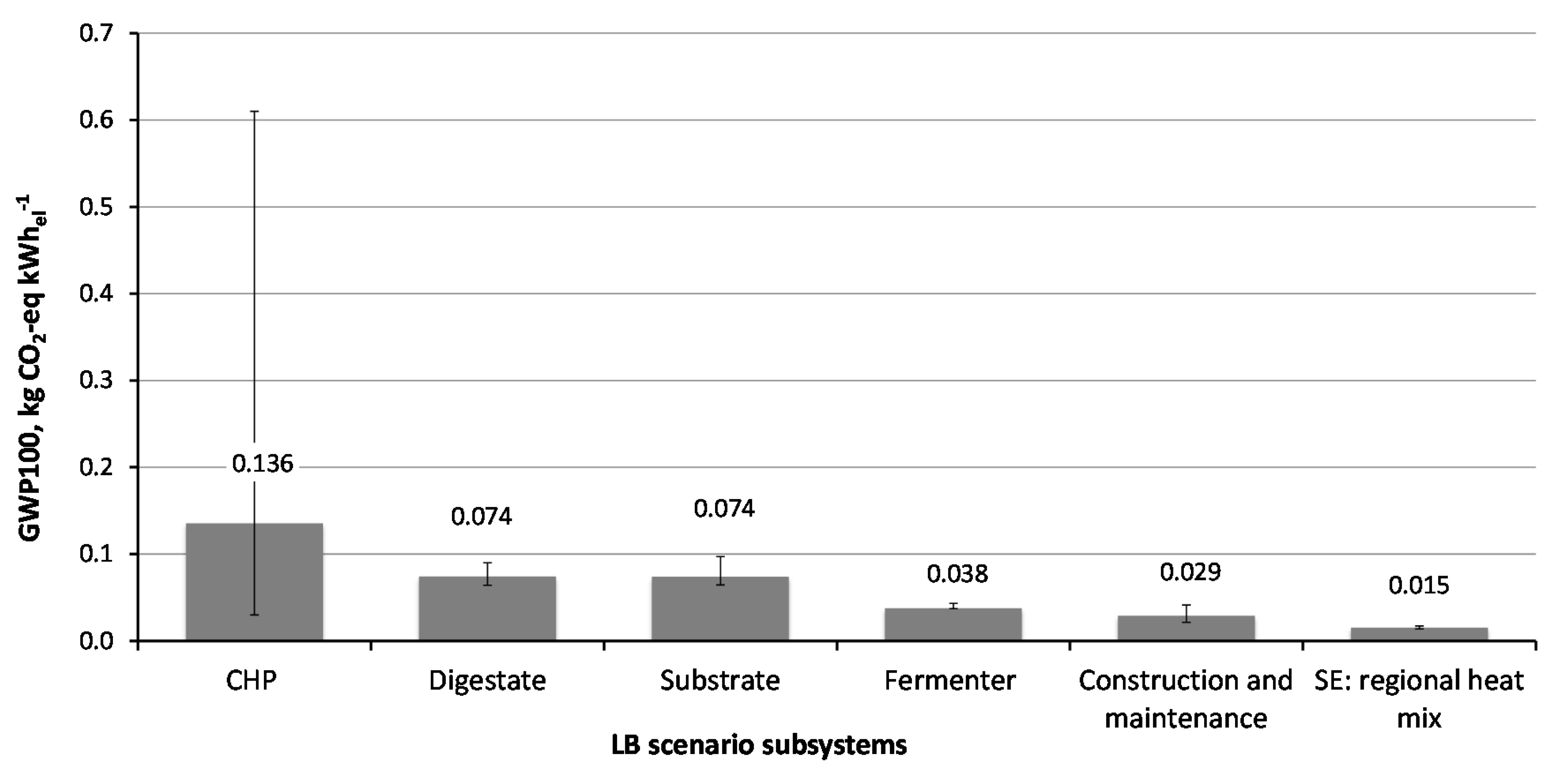
3.3.1. Climate Change Impacts

In contrast to the SQ scenario, the LB scenario uses much more substrate and generates much more biogas, and this explains most of the LB scenario’s main contributions. Its climate change impact (Figure 5) is dominated by methane slip from the much larger biogas CHP (37% of overall emissions, or 0.136 kg CO2-eq kWhel−1), followed by digestate application emissions and by the production and processing of substrates (20% or 0.074 kg CO2-eq kWhel−1 each). The methane slip contribution is within the range reported by a large-scale monitoring study of 16 biogas plants [41]. Impacts due to digestate management occur mainly in the form of methane and nitrous oxide emissions (45% and 39% of digestate GWP, respectively), and almost all the rest (15% of digestate GWP) is due to CO2 from transport, separation, and spreading machinery operation. Most substrate-related emissions stem from hay production (76% of substrate GWP, or 0.056 kg CO2-eq kWhel−1) and are mainly caused by agricultural machinery operation. By comparison, Gerin et al. [43] calculated only 0.022 kg CO2-eq kWhel−1 for grass silage production for farm-scale biogas electricity in the Belgian Ardennes, using extensive grassland harvested for biodiversity conservation. However, they assume a yield that is more than double that of this study’s alpine grassland, and hay requires more machinery use than grass silage. Further contributions to the LB scenario’s GWP include: emissions due to biogas fermenter operations (10% of total GWP or 0.038 kg CO2-eq kWhel−1), biogas plant construction and maintenance (8% or 0.029 kg CO2-eq kWhel−1), and SE heat (4% or 0.015 kg CO2-eq kWhel−1).

3.3.2. Other Impact Categories

In contrast to the LB climate change contribution, biogas CHP emissions contribute little to the other five impact categories studied. Instead, hay production, biogas plant infrastructure, and digestate management contribute the most. The largest portion of the LB scenario’s non-renewable energy demand (48% or 1.1 MJ-eq kWhel−1) is linked to emissions during fuel combustion for hay substrate production and transport, followed by energy consumption for construction materials production (18% or 0.4 MJ-eq kWhel−1).
LB freshwater ecotoxicity impacts are predominantly due to bromine emissions from crude oil production, again for fuel consumed during hay substrate production (39% or 2.08 × 10⁻⁵ kg 1,4-DCB-eq kWhel−1) and for mastic asphalt surfaces at the biogas plant (17% or 9.14 × 10⁻⁶ 1,4-DCB-eq kWhel−1).
Human toxicity impacts are largely caused by the production of infrastructure for hay production (roughage storage facility including a hay blower and a telescopic spreader; 45% or 0.009 kg 1,4-DCB-eq kWhel−1) and by construction materials for the biogas plant (27% or 0.005 kg 1,4-DCB-eq kWhel−1). These impacts can be traced back to production wastes for copper used in the various materials, including arsenic (26% of total impacts), lead (17%), and mercury (16%).
Most of the overall terrestrial acidification impacts (66% or 0.010 kg SO2-eq kWhel−1) and particulate matter formation (48% or 0.0013 kg PM10-eq kWhel−1) are caused by digestate management, mainly from ammonia emissions.
There is a statistically significant difference between most of the six LB scenario subsystems over the six impact categories evaluated. Between digestate management and the production/processing of substrates, no significant difference was found for the climate change impact category.

3.4. Sensitivity Analyses

Two key modeling assumptions were tested for their effect on the impact assessment outcomes. The first sensitivity analysis replaces the regional electricity mix with the national Austrian grid electricity mix (consumption at mid-voltage including imported electricity), both for the SE electricity and for the biogas plant operation. The national Austrian mix has a much higher carbon footprint than the regional mix (0.411 CO2-eq kWhel−1 versus 0.185 CO2-eq kWhel−1). Substituting the national Austrian mix adds 0.212 kg CO2-eq kWhel−1 (or 42%) to the total GWP of the SQ scenario (0.713 versus the original 0.501 CO2-eq kWhel−1) and 0.030 CO2-eq kWhel−1 (or 8%) to the total GWP of the LB scenario (0.397 versus the original 0.367 kg CO2-eq kWhel−1). As is to be expected, a higher carbon footprint for grid electricity affects mostly the SE consumption in the SQ scenario and thus increases the advantage of the LB scenario in terms of climate impact. Vo et al. [14] also found the used electricity mix to be crucial for the performance of power to gas systems upgrading biogas produced from grass and slurry.
The second sensitivity analysis alters the local SE heat system in the SQ scenario that is assumed to be replaced by the LB scenario’s CHP off-heat. Originally, this local SE heat is oil-fired residential heating that is common in the municipality. In the first alternative, a worst case for the LB scenario is that it is not able to market the biogas CHP off-heat at all. Consequently, the SQ scenario would not need to match off-heat by including a local SE heat mix, and this would reduce the overall SQ GWP dramatically from 0.501 to 0.256 kg CO2-eq kWhel−1, which is only 70% of the LB scenario’s GWP. This clearly demonstrates the importance for biogas energy of using CHP off-heat. Bacenetti et al. [44] also emphasize that the utilization of waste heat can significantly improve the GWP of biogas electricity. In the second alternative assumption, CHP off-heat in the LB scenario is assumed to be marketed again, but the matching SE heat in the SQ scenario is only partially assumed to come from oil-fired residential heating systems, with the remaining heat coming from wood-chip fired district heating. In the extreme, modeling the SQ scenario with all SE heat from wood-chip fired district heating (and none from oil-fired heating) would also lead to a much reduced GWP (from 0.501 to 0.270 kg CO2-eq kWhel−1), only 74% of the LB GWP. Figure 6 compares the overall scenario GWPs under this alternative assumption, as the shares of replaced heat in the SQ scenario change from all wood-chip heat and no heating oil to the opposite. For a GWP advantage of the LB scenario over the SQ scenario, a minimum of 42% of the CHP heat used off-site would have to replace heating oil (and a maximum of 58% would replace wood-chips). This threshold percentage is a low estimate, since it is based on the median GWP and does not account for the uncertainty of the two systems. Evangelisti et al. [45] also report that the most critical assumption for the LCA of large-scale food waste digestion concerns the quantity and composition of the energy substituted by the biogas energy. A detailed model for the most likely future energy system in the municipality is outside the scope of this study, but it would require a careful evaluation of the number of homes and enterprises likely to switch their heating systems, and a detailed analysis of any integration of CHP off-heat into the existing local district heating operations. For example, the LB plant could allow the district heating system to shut down during off-peak months, preventing its operation at inefficient partial loads and thus reducing pollutant emission factors.

4. Conclusions

Locally produced biogas (LB) energy, fed by steam-explosion pretreated hay from previously abandoned grassland and by local organic wastes, has a significantly lower environmental impact in three out of six studied categories than the current status quo (SQ) biogas scenario, where the grassland biomass is not utilized and only local organic wastes generate biogas in a regional waste treatment center. A life cycle assessment based on system expansion compares the environmental impacts of generating equal amounts of electricity and heat from both systems. The LB scenario’s GWP (0.367 kg CO2-eq kWhel−1) is found to be significantly lower, only 73% of the SQ scenario’s GWP (0.501 kg CO2-eq kWhel−1). Even more pronounced advantages of the LB scenario relative to the SQ scenario are found in two other impact categories, non-renewable cumulative energy demand and freshwater ecotoxicity, with LB impacts only 40% and 42%, respectively, of the SQ impacts.
The main reason for the SQ scenario’s disadvantage in these impact categories is the fossil fuels required to match the energy output of the LB scenario’s biogas CHP. By contrast, the LB scenario’s GWP is dominated by methane slip from the CHP unit, followed by emissions during digestate management and during hay production from grassland.
The comparison between the two scenarios is not entirely favorable for the LB scenario: in two impact categories—terrestrial acidification and particulate matter formation—the LB scenario has substantially higher environmental impacts, at 341% and 319% of the SQ impacts, respectively. Both categories are dominated by ammonia emissions during the storage and field application of much larger amounts of digestate than in the SQ scenario. In the last category studied—human toxicity—impacts are comparable for both scenarios. In the SQ scenario, they are caused by the SE electricity mix but, in the LB scenario, by infrastructure production (hay production equipment and biogas plant construction materials).
A sensitivity analysis of the GWP confirms the critical importance of the LCA model’s energy system assumptions: replacing the renewables-heavy local electricity mix with a more carbon-intensive national grid mix increases the SQ GWP by 42%, but the LB GWP increases only by 8%, thus emphasizing the LB scenario’s advantage. Assumptions about which SE heat source in the SQ scenario is replaced in the LB scenario by marketed biogas CHP off-heat can even change which scenario has the lower GPW: when the replaced heat source is renewable (district heat from wood-chips) instead of fossil (residential oil furnaces), the SQ scenario’s GWP is substantially reduced, to only 74% of the LB scenario’s climate impact, respectively. If the LB off-heat cannot be marketed at all, the SQ scenario also gains an advantage, with its GWP being only 70% of the LB GWP. The GWP is comparable for both scenarios if at least 42% of the LB scenario’s marketed CHP off-heat replaces residential oil furnaces in the SQ scenario, and the remainder replaces district heat from wood-chips.
In summary, under the assumptions made in the study, a hypothetical local biogas production from abandoned alpine grassland and from local organic wastes can be expected to reduce greenhouse gas emissions and to preserve alpine grassland, if partially at the expense of other environmental impacts. These findings are especially relevant to local decision-makers who wish to move towards more sustainable local energy sources.

Supplementary Materials

The following are available online at https://www.mdpi.com/2071-1050/12/23/9945/s1, Table S1: Digestate emissions, Electricity mix Vorarlberg, Heat mix Vorarlberg.

Author Contributions

Conceptualization, I.K. and G.P.; methodology, I.K. and G.P.; software, I.K. and M.K.S.; validation, I.K., M.K.S. and G.P.; formal analysis, I.K., J.L. and G.P.; investigation, I.K.; M.K.S., A.B.; and G.P.; resources, A.B. and A.G.; data curation, I.K., J.L. and M.K.S.; writing—original draft preparation, I.K., M.K.S. and G.P.; writing—review and editing, I.K., G.P. and A.B.; visualization, I.K. and M.K.S.; supervision, G.P., A.G. and A.B.; project administration, A.B.; funding acquisition, A.G. and A.B.; All authors have read and agreed to the published version of the manuscript.

Funding

This work was supported by the COMET (Competence Centers for Excellent Technologies) program at the alpS GmbH—Centre for Climate Change Adaptation [grant number 26030 E03]. The program is an initiative of the Federal Ministry of Transport, Innovation and Technology and the Federal Ministry of Science, Research and Economy. Additional support for the program comes from the federal states of Tyrol and Vorarlberg. The program is administered by the Austrian Research Promotion Agency (FFG).

Acknowledgments

Open access funding provided by BOKU Vienna Open Access Publishing Fund.

Conflicts of Interest

The authors declare no conflict of interest.

References

  1. Schermer, M. REsilience of Marginal GrAssland and Biodiversity Management Decision Support—REGARDS; Department of Sociology, University Innsbruck: Innsbruck, Austria, 2015. [Google Scholar]
  2. Kral, I.; Piringer, G.; Saylor, M.; Gronauer, A.; Bauer, A. Environmental effects of steam explosion pretreatment on biogas from maize-case study of a 500-kW Austrian biogas facility. Bioenergy Res. 2016, 9, 198–207. [Google Scholar] [CrossRef]
  3. Bauer, A.; Lizasoain, J.; Theuretzbacher, F.; Agger, J.W.; Rincón, M.; Menardo, S.; Saylor, M.K.; Enguídanos, R.; Nielsen, P.J.; Gronauer, A.; et al. Steam explosion pretreatment for enhancing biogas production of late harvested hay. Bioresour. Technol. 2014, 166, 403–410. [Google Scholar] [CrossRef] [PubMed]
  4. Ferreira, L.C.; Donoso-Bravo, A.; Nilsen, P.J.; Fdz-Polanco, F.; Perez-Elvira, S.I. Influence of thermal pretreatment on the biochemical methane potential of wheat straw. Bioresour. Technol. 2013, 143, 251–257. [Google Scholar] [CrossRef] [PubMed]
  5. Schumacher, B.; Wedwitschka, H.; Hofmann, J.; Denysenko, V.; Lorenz, H.; Liebetrau, J. Disintegration in the biogas sector—Technologies and effects. Bioresour. Technol. 2014, 168, 2–6. [Google Scholar] [CrossRef]
  6. Sapci, Z.; Morken, J.; Linjordet, R. An Investigation of the Enhancement of Biogas Yields from Lignocellulosic Material using Two Pretreatment Methods: Microwave Irradiation and Steam Explosion. BioResources 2013, 8, 1976–1985. [Google Scholar] [CrossRef]
  7. Risberg, K.; Sun, L.; Leven, L.; Horn, S.J.; Schnurer, A. Biogas production from wheat straw and manure—impact of pretreatment and process operating parameters. Bioresour. Technol. 2013, 149, 232–237. [Google Scholar] [CrossRef]
  8. Pérez-Elvira, S.I.; Fdz-Polanco, F. Continuous thermal hydrolysis and anaerobic digestion of sludge. Energy integration study. Water Sci. Technol. 2012, 65, 1839–1846. [Google Scholar] [CrossRef]
  9. Li, A.; Antizar-Ladislao, B.; Khraisheh, M. Bioconversion of municipal solid waste to glucose for bio-ethanol production. Bioprocess Biosyst. Eng. 2007, 30, 189–196. [Google Scholar] [CrossRef]
  10. Sargalski, W.; Solheim, O.E.; Fjordside, C. Treating Organic Waste with CAMBI® THP. In Proceedings of the 12th European Biosolids and Organic Resources Conference, Manchester, UK, 12–14 November 2007. [Google Scholar]
  11. Shafiei, M.; Kabir, M.M.; Zilouei, H.; Horváth, I.S.; Karimi, K. Techno-economical study of biogas production improved by steam explosion pretreatment. Bioresour. Technol. 2013, 148, 53–60. [Google Scholar] [CrossRef]
  12. Finkbeiner, M.; Inaba, A.; Tan, R.; Christiansen, K.; Klüppel, H.-J. The New International Standards for Life Cycle Assessment: ISO 14040 and ISO 14044. Int. J. Life Cycle Assess. 2006, 11, 80–85. [Google Scholar] [CrossRef]
  13. Bedoić, R.; Čuček, L.; Ćosić, B.; Krajnc, D.; Smoljanić, G.; Kravanja, Z.; Ljubas, D.; Pukšec, T.; Duić, N. Green biomass to biogas—A study on anaerobic digestion of residue grass. J. Clean. Prod. 2019, 213, 700–709. [Google Scholar] [CrossRef]
  14. Vo, T.T.Q.; Rajendran, K.; Murphy, J.D. Can power to methane systems be sustainable and can they improve the carbon intensity of renewable methane when used to upgrade biogas produced from grass and slurry? Appl. Energy 2018, 228, 1046–1056. [Google Scholar] [CrossRef]
  15. Wang, L.; Littlewood, J.; Murphy, R.J. Environmental sustainability of bioethanol production from wheat straw in the UK. Renew. Sustain. Energy Rev. 2013, 28, 715–725. [Google Scholar] [CrossRef] [Green Version]
  16. Prasad, A.; Sotenko, M.; Blenkinsopp, T.; Coles, S.R. Life cycle assessment of lignocellulosic biomass pretreatment methods in biofuel production. Int. J. Life Cycle Assess. 2015, 21, 44–50. [Google Scholar] [CrossRef] [Green Version]
  17. Schumacher, B.; Oechsner, H.; Senn, T.; Jungbluth, T. Life cycle assessment of the conversion of Zea mays and x Triticosecale into biogas and bioethanol. Eng. Life Sci. 2010, 10, 577–584. [Google Scholar] [CrossRef]
  18. Ingrao, C.; Bacenetti, J.; Adamczyk, J.; Ferrante, V.; Messineo, A.; Huisingh, D. Investigating energy and environmental issues of agro-biogas derived energy systems: A comprehensive review of Life Cycle Assessments. Renew. Energy 2019, 136, 296–307. [Google Scholar] [CrossRef]
  19. Frühauf, S. Potentialanalyse Biogener Roh-, Rest-und Abfallstoffe für die Einbringung in eine Biogasanlage in der Gemeinde Lech am Arlberg. Master’s Thesis, University of Natural Resources and Life Sciences, Vienna, Austria, 2013. [Google Scholar]
  20. Bayerische Landesanstalt für Landwirtschaft (2014) Biogasausbeuten verschiedener Substrate. Available online: http://www.lfl.bayern.de/iba/energie/049711/ (accessed on 20 October 2020).
  21. Ecoinvent Centre. Ecoinvent Data v 2.2. Swiss Centre for Life Cycle Inventories, Dübendorf. 2014. Available online: https://www.ecoinvent.org/database/older-versions/ecoinvent-version-2/ecoinvent-version-2.html (accessed on 22 October 2020).
  22. Amon, B.; Amon, T.; Boxberger, J.; Alt, C. Emissions of NH3, N2O and CH4 from dairy cows housed in a farmyard manure tying stall (housing, manure storage, manure spreading). Nutr. Cycl. Agroecosystems 2001, 60, 103–113. [Google Scholar] [CrossRef]
  23. Energie, A.d.V.L.-B. Energie-zukunft Vorarlberg—Ergebnisse aus dem Visionsprozess. In Schritt für Schritt zur Energieautonomie. Quantifizierungen und Zukunftsentwürfe; Amt der Vorarlberger Landesregierung: Bregenz, Austria, 2010; pp. 1–22. [Google Scholar]
  24. Landesregierung, A.d.V. Energiebericht 2013 auf Basis der Energieverbrauchsdaten 2012; Amt der Vorarlberger Landesregierung: Bregenz, Austria, 2013; pp. 1–18. [Google Scholar]
  25. Kaltschmitt, M.; Streicher, W. Regenerative Energien in Österreich: Grundlagen, Systemtechnik, Umweltaspekte, Kostenanalysen, Potenziale, Nutzung, 1st ed.; Vieweg + Teubner: Wiesbaden, Germany, 2009. [Google Scholar]
  26. Biermayr, P.; Eberl, M.; Ehrig, R.; Fechner, H.; Kristöfel, C.; Neuhauser, P.E.; Prüggler, N.; Sonnleitner, A.; Strasser, C.; Weiss, W.; et al. Innovative Energietechnologien in Österreich- Marktentwicklung 2011. Biomasse, Photovoltaik, Solarthermie und Wärmepumpen; Federal Ministry of Agriculture, Forestry, Environment and Water Management: Vienna, Austria, 2012; p. 171.
  27. Döhler, H.; Eckel, H.; Fröba, N.; Grebe, S.; Hartmann, S.; Häußermann, U.; Klages, S.; Sauer, N.; Nakazi, S. Faustzahlen Biogas, 2nd ed.; Kuratorium für Technik und Bauwesen in der Landwirtschaft e.V. (KTBL): Darmstadt, Germany, 2009; p. 236. [Google Scholar]
  28. Frühauf, S.; Saylor, M.K.; Lizasoain, J.; Gronauer, A.; Bauer, A. Potential Analysis of Agro-Municipal Residues as a Source of Renewable Energy. BioEnergy Res. 2015, 8, 1449–1456. [Google Scholar] [CrossRef]
  29. Laaber, M. Gütesiegel Biogas. Evaluierung Der Technischen, ökologischen und Sozioökonomischen Rahmenbedingungen für eine Ökostromproduktion aus Biogas. Ph.D. Thesis, University of Natural Resources and Life Sciences, Vienna, Austria, 2011. [Google Scholar]
  30. Cuhls, C.; Mähl, D.B.; Berkau, S.; Clemens, P.D.J. Ermittlung der Emissionssituation bei der Verwertung von Bioabfällen; Gewitra-Ingenieurgesellschaft für Wissenstransfer mbH: Bonn, Germany, 2008; pp. 1–172. [Google Scholar]
  31. Lampert, C.; Tesar, M.; Thaler, P. Klimarelevanz und Energieeffizienz der Verwertung biogener Abfälle; 9783990041567; Umweltbundesamt GmbH: Vienna, Austria, 2011; pp. 3–76. [Google Scholar]
  32. Wulf, S.; Maeting, M.; Clemens, J. Application technique and slurry co-fermentation effects on ammonia, nitrous oxide, and methane emissions after spreading: II. Greenhouse gas emissions. J. Environ. Qual. 2002, 31, 1795–1801. [Google Scholar] [CrossRef]
  33. Amon, B.; Kryvoruchko, V.; Amon, T.; Zechmeister-Boltenstern, S. Methane, nitrous oxide and ammonia emissions during storage and after application of dairy cattle slurry and influence of slurry treatment. Agric. Ecosyst. Environ. 2006, 112, 153–162. [Google Scholar] [CrossRef]
  34. Buchgraber, K.; Gindl, G. Zeitgemäße Grünlandbewirtschaftung; Stocker Verlag: Graz, Austria, 2004. [Google Scholar]
  35. Gmb, H.G.D. OpenLCA 1.8; Green Delta GmbH: Berlin, Germany, 2014. [Google Scholar]
  36. Goedkoop, M.J.; Reinout, H.; Huijbregts, M.; De Schryver, A.; Struijs, J.; Van Zelm, R. ReCiPe 2008, a Life Cycle Impact Assessment Method Which Comprises Harmonised Category Indicators at the Midpoint and Endpoint Level, 1st ed.; Report I: Characterisation; Ministerie van VROM: Den Haag, The Netherlands, 2008. [Google Scholar]
  37. Huijbregts, M.A.J.; Steinmann, Z.J.N.; Elshout, P.M.F.; Stam, G.; Verones, F.; Vieira, M.D.M.; Hollander, A.; Van Zelm, R. ReCiPe2016: A Harmonized Life Cycle Impact Assessment Method at Midpoint and Endpoint Level. RIVM Report 2016-0104; National Institute for Public Health and the Environment: Bilthoven, The Netherlands, 2016. [Google Scholar]
  38. Frischknecht, R.; Jungbluth, N.; Althaus, H.-J.; Bauer, C.; Doka, G.; Dones, R.; Hirschier, R.; Hellweg, S.; Humbert, S.; Köllner, T.; et al. Implementation of Life Cycle Impact Assessment Methods. Ecoinvent Report No. 3, v2.0; Frischknecht, R., Jungbluth, N., Eds.; Swiss Centre for Life Cycle Inventories: Dübendorf, Switzerland, 2007; p. 151. [Google Scholar]
  39. IBM Corp. IBM SPSS Statistics for Windows, Version 21.0; IBM: New York, NY, USA, 2012. [Google Scholar]
  40. Siegl, S. Öko-Strom aus Biomasse. Vergleich der Umweltwirkungen verschiedener Biomasse-Technologien zur Stromerzeugung Mittels Lebenszyklusanalysen. Ph.D Thesis, University of Natural Resources and Life Sciences, Vienna, Austria, 2010. [Google Scholar]
  41. Bachmaier, J. Treibhausgasemissionen Und Fossiler Energieverbrauch Landwirtschaftlicher Biogasanlagen. Eine Bewertung auf Basis von Messdaten mit Evaluierung der Ergebnisunsicherheit mittels Monte-Carlo-Simulation. Ph.D. Thesis, University of Natural Resources and Life Sciences, Vienna, Austria, 2012. [Google Scholar]
  42. Pucker, J.; Jungmeier, G.; Siegl, S.; Potsch, E.M. Anaerobic digestion of agricultural and other substrates—implications for greenhouse gas emissions. Animal 2013, 7 (Suppl. 2), 283–291. [Google Scholar] [CrossRef] [PubMed]
  43. Gerin, P.A.; Vliegen, F.; Jossart, J.M. Energy and CO2 balance of maize and grass as energy crops for anaerobic digestion. Bioresour. Technol. 2008, 99, 2620–2627. [Google Scholar] [CrossRef] [PubMed]
  44. Bacenetti, J.; Sala, C.; Fusi, A.; Fiala, M. Agricultural anaerobic digestion plants: What LCA studies pointed out and what can be done to make them more environmentally sustainable. Appl. Energy 2016, 179, 669–686. [Google Scholar] [CrossRef] [Green Version]
  45. Evangelisti, S.; Lettieri, P.; Borello, D.; Clift, R. Life cycle assessment of energy from waste via anaerobic digestion: A UK case study. Waste Manag. 2014, 34, 226–237. [Google Scholar] [CrossRef]
Figure 1. System diagram of status quo (SQ) scenario. System expansion processes are added to maintain functional equivalence with the local biogas (LB) system (see Figure 2). For simplicity, upstream processes are not shown in the system expansion part.
Sustainability 12 09945 g001
Figure 2. System diagram of local biogas (LB) production scenario. System expansion processes are added to maintain functional equivalence with the status quo (SQ) system (see Figure 1). For simplicity, upstream processes are not shown in the system expansion part.
Sustainability 12 09945 g002
Figure 3. Comparison of relative impacts of the SQ and LB scenario. Higher impact for a category = 100%.
Sustainability 12 09945 g003
Figure 4. Contribution of subsystems to status quo (SQ) scenario, climate change impact category. Error bars: 5th–95th interpercentile range, based on 1000 Monte Carlo simulations. SE = system expansion subsystems (heat, electricity, and manure treatment); CHP = methane slip from exhaust; substrate = transportation of substrates.
Sustainability 12 09945 g004
Figure 5. Contribution of subsystems to status quo (LB) scenario, climate change impact category. Error bars: 5th–95th interpercentile range, based on 1000 Monte Carlo simulations. SE = system expansion subsystems (heat and electricity).
Sustainability 12 09945 g005
Figure 6. Sensitivity of SQ scenario total GWP to changes in assumed SQ system expansion heat source (total local SE heat = heating oil share + share of wood-chip-fueled district heating).
Sustainability 12 09945 g006
Table 1. Annual substrate inputs and methane and energy yields in the case study scenarios. In the LB scenario, hay and manure are added to currently used SQ substrates to allow operation of a 500 kWel biogas plant [3,20]. FM = fresh matter, DM = dry matter, SEP = steam explosion pretreatment.
Substrate InputsSubstrateDM Content Organic DM ContentAnnual CH4 yieldAnnual Energy from CH4
[t FM a−1][% of FM][% of DM][Nm3 a−1][kWh a−1]
Status Quo (SQ) Scenario
To biogas without SEP
 Municipal organic waste mixture 89439%52%55,772555,492
 Oils and fats 3695%92%21,396213,099
Direct to composting
 Green cuttings6015%89%n/an/a
Direct to field application
 Solid manure263025%80%n/an/a
Total SQ Scenario (biogas only)930 77,168768,591
Local Biogas (LB) Scenario
To biogas with SEP
 Hay 337187%94%762,6637,596,119
 Municipal organic waste mixture 89439%52%71,108708,234
 Oils and fats 3695%92%21,396213,099
 Green cuttings6015%89%221722,084
To biogas without SEP
 Solid manure263025%80%129,4591,289,410
Total LB Scenario (biogas only)6991 986,8429,828,947
Table 2. Annual electricity and heat outputs for the two scenarios. Scenario outputs were equalized with system expansion (SE) processes to ensure functional equivalence.
Energy [kWh a−1]Status Quo (SQ) ScenarioLocal Biogas (LB) Scenario
Electricity
CHP electricity, total output292,0653,735,000
SE electricity3,442,935 an/a
Expanded system electricity output (CHP electricity output plus SE electricity)3,735,0003,735,000
Heat
CHP heat, total output322,8084,128,158
CHP heat used on-site37,123549,239
CHP heat used off-site258,247 b2,807,147
CHP heat output not used27,439276,392
SE heat2,807,147 c258,247 d
Expanded system heat used off-site (CHP heat used off-site plus SE heat)3,065,3943,065,394
Note: a balances LB electricity for equal electricity output, based on regional electricity mix [23,24]. b authors’ assumptions: 80% of CHP heat sent to off-site use in both scenarios. LB off-site heat is reduced by 15% due to district heat transfer losses [25], SQ amount assumes consumption near regional waste treatment plant and neglects heat transfer losses. c balances LB heat used off-site in the municipality; based on residential heating oil systems. d balances SQ heat used off-site near regional waste treatment plant; based on regional heat mix [23,24].
Table 3. Life cycle impact assessment results—scenario comparison by impact category.
SQ ScenarioLB ScenarioLB Impacts in % of SQ Impacts
Impact CategoryReference UnitPoint Estimate5th-Percentile95th-PercentilePoint Estimate5th-Percentile95th-Percentile
Climate changekg CO2-eq kWh−15.01 × 10−14.56 × 10−15.69 × 10−13.67 × 10−12.63 × 10−18.55 × 10−173%
Non-renewable energy resourcesMJ-eq kWh−15.534.856.302.221.932.6840%
Freshwater ecotoxicitykg 1,4-DCB-eq kWh−11.26 × 10−46.16 × 10−52.36 × 10−45.33 × 10−52.89 × 10−59.44 × 10−542%
Human toxicity kg 1,4-DCB-eq kWh−11.88 × 10−21.18 × 10−23.01 × 10−21.99 × 10−21.34 × 10−23.09 × 10−2106%
Terrestrial acidificationkg SO2-eq kWh−13.78 × 10−31.89 × 10−35.71 × 10−31.48 × 10−25.03 × 10−32.47 × 10−2393%
Particulate matter formationkg PM10-eq kWh−17.26 × 10−44.78 × 10−49.81 × 10−42.69 × 10−31.41 × 10−33.99 × 10−3371%
Publisher’s Note: MDPI stays neutral with regard to jurisdictional claims in published maps and institutional affiliations.

