Abstract
The increasing complexity of the design and operation evaluation process of multi-energy grids (MEGs) requires tools for the coupled simulation of power, gas and district heating grids. In this work, we analyze a number of applicable tools and find that most of them do not allow coupling of infrastructures, oversimplify the grid model or are based on inaccessible source code. We introduce the open source piping grid simulation tool pandapipes that—in interaction with pandapower—addresses three crucial criteria: clear data structure, adaptable MEG model setup and performance. In an introduction to pandapipes, we illustrate how it fulfills these criteria through its internal structure and demonstrate how it performs in comparison to STANET®. Then, we show two case studies that have been performed with pandapipes already. The first case study demonstrates a peak shaving strategy as an interaction of a local electricity and district heating grid in a small neighborhood. The second case study analyzes the potential of a power-to-gas device to provide flexibility in a power grid while considering gas grid constraints. These cases show the importance of performing coupled simulations for the design and analysis of future energy infrastructures, as well as why the software should fulfill the three criteria.
1. Introduction
Considering the new strategic view on the policy area “Clean Energy” within the European Green Deal [1]—a roadmap towards a sustainable economy developed by the European Commission—the energy infrastructure in Europe is expected to change drastically over the next years. On the one hand, the Hydrogen Strategy [2] is meant to promote the emergence of a hydrogen infrastructure that complements and partially replaces the existing natural gas infrastructure. The Energy System Integration Strategy [3], on the other hand, aims at an increased interconnection of energy sectors and markets. It describes an energy infrastructure design that allows consumer needs to be satisfied through different energy carriers, thereby increasing its overall efficiency and resilience. These targeted changes will increase the complexity of the energy system as a whole.
As of today, different energy infrastructures are designed and operated independently from each other. Unlocking the potential of sector integration requires a “new, holistic approach for both large-scale and local infrastructure planning” [3]. Methods and tools for infrastructure design need to reflect the increased complexity in order to address many challenges on all scales and in all parts of the energy system design [4]. Challenges will occur in the following fields:
- Assessment of supply options with different energy infrastructures: With increasing interconnection of infrastructures, how energy is supplied to end consumers can vary greatly. For instance, Then et al. [5] gave an overview of studies on the controversial role of the natural gas infrastructure and elaborated on the effects that a decline in energy demand can have on grid charges. In [6], they put forward that increasing grid charges could accelerate gas grid defection as a self-induced effect. Kisse et al. [7] investigated the effects that changes in heating technologies for residential buildings have on investments into electrical and gas grid expansion as well as on CO2-emissions. To improve the prediction of suitable supply scenarios for network operators in a multi-energy system (MES), methods and models have to consider all energy infrastructures in a combined optimization approach.
- Grid integration and expansion in coupled energy infrastructures: The progressive electrification and renewable generation increases both load and generation in distribution grids. All new devices and power plants must be integrated on the respective voltage level which often spurs network operators to expand or re-design their power grids. In the future, this planning process needs to address the increasing interconnection to other infrastructures and new opportunities for trading flexibility or storing energy [8]. Approaches should consider the possibility to rededicate parts of the infrastructure to other carriers or even dismantle infrastructure that is no longer required [2,5]. It is crucial to identify suitable investment paths toward a future supply infrastructure taking into account the longevity and high capital expenditure of infrastructure assets. These challenges also have to be reflected by large-scale grid integration and expansion studies (e.g., [9,10]).
- Analysis and optimization of operation strategies: Sector coupling facilities, such as combined heat and power (CHP) plants, heat pumps or power-to-gas (P2G) devices, are expected to deliver ancillary services for power system operation (e.g., frequency support, voltage support, congestion management, etc.). Although such services are mainly required in the power grid, operation strategies should be optimized by respecting the operational constraints of all connected infrastructures. For example, Liu et al. [11] analyzed different operation modes of CHP plants and how they influence power and gas grid constraints. In [12], an optimal power flow (OPF) implementation is presented that includes constraints from the gas grid as side conditions.
- Urban planning: The planning phase of new districts offers great potential for low-cost decarbonized energy supply by implementing small MESs with optimized grid infrastructure [13]. To address arising challenges of urban planning, the spatial and energy infrastructure planning need to be interconnected [14]. Forming so-called energy communities with high shares of renewable energy sources (RES) and local trading capabilities can play an important role in increasing energy efficiency and is therefore incentivized by the European Union [15]. In such small systems, choosing and optimizing the operation strategy is crucial in order to use energy locally or to offer ancillary services to the external power grid [16].
- Market design: If sector coupling facilities deliver flexibilities or other ancillary services, they also need to be remunerated. Mancarella et al. [17] suggested an approach to determine the profitability of MES, which deliver ancillary services, by considering the revenue and the cost of energy shifting. With an increased interest in local energy markets [18] comes a need to analyze approaches with respect to the technical and economic performance. For such analyses, the complex state of the whole MES and market mechanisms need to be modeled.
The challenges described above require powerful tools for coupled multi-energy grid (MEG) simulation and optimization. Several modeling and optimization approaches are presented in [19] (and the references cited therein). In this work, we introduce the open source tool pandapipes which is meant to simulate stationary and quasi-stationary flows in pipes, considering hydraulic and thermal properties of the flowing fluid. It complements the open source power system analysis tool pandapower [20], as it is based on the same structure and implements similar core methods, such as the Newton–Raphson solver. The two tools can be combined into a powerful and easy-to-use MEG simulation environment with the help of the pandapipes multi-energy module. As both tools are published under the terms of a 3-clause BSD license, they can be used by anyone for any purpose free of charge. Since pandapipes is based on Python, this tool can be combined with any other Python package for further analysis. For instance, there are interfaces to NetworkX [21] for topology analysis, to matplotlib [22] for plotting and to geopandas [23] for processing geographical information. All these characteristics enhance the potential of pandapipes to automate processes and easily adapt models and simulation setups. Therefore, pandapipes is well suited to address the challenges of energy infrastructure analysis and planning. Since the coupling with pandapower is very simple, many use cases that have already been addressed with pandapower can be adopted to an integrated approach.
In the present work, we want to evaluate the innovative potential of pandapipes. Section 2 gives an overview over different approaches to MEG simulation and derives three criteria to be addressed by a dedicated tool: clear data structure, adaptable MEG model setup and performance. Section 3 introduces pandapipes and describes its structure and model implementations, thereby illustrating how these criteria are addressed. Section 4 demonstrates two use cases that were implemented with the help of pandapipes. In the first use case, we analyze local peak shaving strategies with the help of a heat pump connected to a district heating grid. We show that operation strategies and their effect on all involved networks can be examined by applying the combination of pandapower and pandapipes. In the second use case, we analyze the potential of P2G devices to reduce congestion in a power grid without violating constraints of the connected gas grid. The presented simulation approach enables large-scale analyses on the effectiveness of P2G devices in different configurations to find a suitable system design. Section 5 concludes on how pandapipes enhances the toolbox of researchers working in the field of MEG analysis and gives insights into possible enhancements to further simplify MEG simulations and to address other types of problems.
2. Multi-Energy Grid Simulation: Overview of Approaches and Requirements
Approaches for the simulation of coupled energy infrastructures can have different levels of detail, making them especially suitable for specific use cases. Thus, a large tool landscape has evolved, of which Table 1 shows an excerpt. We characterize the tools by licensing, modeled infrastructures, model detail and the possibility to conduct coupled simulations, i.e., simulations of power, gas and district heating grids based on a single interlinked model in one simulation run. Of special interest for the research community are open source tools, as they are customizable, automatable and mostly free of charge. Commercial tools usually have a strong focus on the user interface and usability. We distinguish three tool categories: grid simulation (GS) tools, energy system modeling and optimization (ESMO) tools and MEG simulation tools.

Table 1.
Overview of power, gas and district heating simulation tools with their scopes and model implementations.
The characteristic of GS tools is that they offer detailed grid models, sometimes even for different infrastructures, but they cannot be coupled within the simulation. ESMO tools analyze power flows between defined areas with a strong focus on energy balancing. Therefore, they precisely model power plants and devices with their control strategies and characteristics such as efficiency or ramp rates. As they do not provide detailed grid models, they can easily integrate all infrastructures within one simulation. Such tools can be used for optimal power system design or power plant deployment planning, i.e., in a flexibility market model used for power balancing.
None of those tools offers sophisticated models for integrated infrastructures, as either the grid model is simplified, or a coupled simulation is not possible. For the simulation of MEGs, two approaches are prominent: Combining dedicated tools with the help of a co-simulation platform and integrating all models in one tool. As pointed out in [24], the main advantage of a co-simulation approach is the possibility of integrating any tool, while leaving the development to the respective experts. Furthermore, distributed simulations can be performed online so that participants can exclude exchange of internal data. Nevertheless, there are also downsides to this approach: Firstly, exchanging data between two or more tools via an external interface is time consuming and usually acts as a bottleneck for complex simulations resolved in space and time. Moreover, the design, functionality and licensing of coupled tools might introduce difficulties for the user to set up the model. Most co-simulation approaches are tailor-made [25] and those with a wider scope might not fit for specific applications [26]. In recent years, dedicated tools were developed for addressing problems in the field of MEG simulation and to overcome the previously mentioned problems of co-simulation. Tools that enable the user to easily run simulations with models for all infrastructure types are rare and have not yet found their way into the open source community, as shown in Table 1.
The main challenge of setting up MEG simulations lies in the complexity of the addressed problems [43]. Therefore, a tool that is designed to solve a multitude of different problems in this field must focus on tackling this challenge, especially considering that user experience might differ greatly. A consistent design is crucial, and the first simple models should be very easy to build, while complex models should be solved efficiently. From these requirements, we derive three criteria that should be addressed by a dedicated tool:
- Clear Data Structure: Mastering the complexity of MEG simulations is only possible if the data is contained in a clearly structured database that allows storing large amounts of data. This is true for the model data of the coupled grids as well as the output data, especially from time series simulations. Many tool descriptions highlight the way data are stored and handled due to convenience and efficiency [20,32,35].
- Adaptable MEG Model Setup: The construction and adaptation of a full simulation model should be simple and efficient. This requires pre-defined, but adaptable models for grid components and sector coupling facilities with their physical properties and respective control strategies. Extensive component libraries are important parts of tools in the area of MEG simulation [38,41]. A permissive open source license is a good precondition to encourage model development [32]. The coupling of simulations for different infrastructures should be as simple as choosing which grids to couple and defining the models for coupling facilities. Different simulation types should be available and combinable, e.g., steady-state, transient or OPF, in order to address different levels of detail of specific use cases.
- Performance: In research, the evaluation of many different setups and use cases is of interest. When performing large-scale studies (e.g., [10]), the simulation time plays an important role to be considered in the design of the tool. From the user’s point of view, it should also be considered that spending a lot of time waiting for calculations to finish can be very inconvenient and inefficient. Model efficiency and simulation speed is therefore also addressed by many tools [20,31,38,40].
As most of the MEG simulation tools introduced in Table 1 are closed-source or based on proprietary software, these criteria are hard to analyze, but some publications give hints. SAInt implements an OPF formulation considering AC power flow equations, transient gas grid equations and coupling terms and is mainly used to analyze outages in coupled transmission grids. A lot of emphasis is put on an increased performance by using a specialized solver. HyFlow implements a power transport formulation for power, gas and heat grids, linked by simplified coupling terms and solved with a Newton–Raphson approach. The field of application is the analysis of power balancing using a cellular approach. MYNTS uses an expression tree formulation of component equations for automatic differentiation, which are solved with non-linear programming solvers. Its main field of application is the evaluation of supply scenarios for gas transport grids, but also coupling terms can be implemented with the generic approach. TransiEnt is a modelica library that defines transient and steady-state equations for the calculation of MES. Its modular approach and different levels of simulation detail allow different simulation setups. Applications have shown the interconnection of operation strategies for different components.
Next to TransiEnt, pandapipes is with its specialized multi-energy module the only MEG simulation tool with an open-source license. Unlike the former, it can even be used without any proprietary software required. It was developed along practical use cases and designed to fulfill the three aforementioned criteria. The multi-energy module integrates pandapipes and pandapower to address challenges in the field of coupled MEG planning and operation. Pandapower has already shown to be well suited as a tool for solving automated planning problems [44], thereby considering different effects such as restoration [45], operation strategies [46] or asset management [47]. It was also used for testing new approaches to contingency analysis [48], curtailment minimization of distributed generators [49], state estimation [50] and fault occurrence evaluation [51]. Its special potential lies in the application within studies that analyze large grid areas in an automated approach, such as grid integration studies [10,52] or energy loss studies [53,54]. Due to its similar design and performance, pandapipes can perform similar studies for piping grids and in combination with pandapower also for MEGs.
3. Overview of Pandapipes
In the previous section, we introduce three criteria for an MEG simulation tool. In the following, we illustrate how pandapipes meets those criteria through a comprehensible design and an efficient calculation method. We introduce the pandapipes grid data structure and the controller architecture, demonstrate how this architecture can be used to build up multi-energy grid simulation models and finally compare the performance of the pipe flow calculation with calculation times of the popular proprietary software STANET®.
3.1. Illustrating Clear Data Structure: Architecture of Pandapipes
In pandapipes, nodes and edges of a network are defined by component models. Every component model introduces equations, describing the physical properties that are solved for. The equations are assembled into a nonlinear system of equations that comply with Kirchhoff’s laws. This system of equations is solved with the Newton–Raphson method. As a result, pandapipes provides pressure values at all nodes in the network and the corresponding flow velocities along the different edges. If a heat grid is modeled, pandapipes also determines temperature values at the nodes. Further properties can be derived from these dependent variables.
3.1.1. The Pandapipes Grid Structure
Different parameters have to be provided by the user to properly set up the mentioned system of equations. The grid model data are stored in a dedicated data structure; the pandapipes net container is shown in Figure 1. It contains pandas tables for different components and additional parameters required to run a simulation, which is an analogy of the pandapower structure. There are two main types of tables: component tables and result tables. Component tables contain all the modeled grid elements with their respective nameplate parameters. For example, the pipe component table contains the two connected junctions along with the parameters length, diameter, roughness and an additional loss coefficient. Those values are required for the hydraulic state simulation. Furthermore, it is possible to set an external heat source or sink, an external temperature and a heat transfer coefficient for the heat transfer calculation. Result tables contain the simulation results for the given component. For some components it is also useful to record geo-information in a separate table. An overview of existing component models in pandapipes is given in Appendix A.
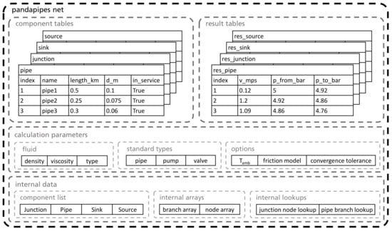
Figure 1.
The pandapipes net and stored data, divided into the groups component tables, result tables, calculation parameters and internal data. The shown data in each group are not exhaustive.
Properties of the operating fluid, such as density for different temperatures and pressures, are stored in the grid container as well. They can be freely defined by the user or chosen from an included fluid library. Other stored parameters are standard types for components, as pumps or pipes, and further options to be set by the user. The available component models are held in a list for each pandapipes net for the internal process. Other internal data include an internal array structure and lookup tables for the conversion between the component tables and the internal structure.
3.1.2. The Pipeflow Procedure
After defining the input data inside the component tables, the calculation can be started by calling the pipeflow function. Figure 2 shows the procedure of the calculation. With the help of the component models, all component tables are transferred to an internal numpy array structure, which is more efficient than the pandas structure, and equations are introduced for the derivatives of the state variables. A connectivity check makes sure that disconnected grid areas are excluded from the calculation. Afterwards, the hydraulic state variables are solved for with the help of a Newton–Raphson solver, which usually requires several iterations to converge. For heat grids, a subsequent heat transfer calculation also uses a Newton–Raphson solver to calculate the node temperatures. In the end, the state variables and derived results are transferred to the result tables.
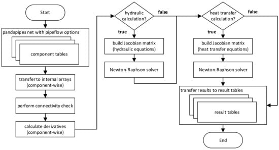
Figure 2.
Flowchart of the pipeflow procedure including hydraulic and heat transfer calculation. The pandapipes net tables serve as interface for the user, while internally an array structure is used for performance reasons.
The most important equations are introduced by branch components which define the pressure loss and the heat transfer model. Node components implement a mass flow or power balance. The mathematics behind the component models in pandapipes and how they are set up into a system of nonlinear equations is presented in Appendix A. In the current version of pandapipes, it is possible to calculate hydraulic properties for compressible and incompressible media and to perform a subsequent heat transfer calculation for incompressible media.
3.1.3. The Controller Architecture and Time Series Simulations
Typically, not only one stationary state is of interest, but instead the grid state has to be observed over a specified period of time, for example a representative day or a full year. For this purpose, pandapipes provides a dedicated function that starts a loop over the time period, as shown in Figure 3. The resolution can be defined by the user and should be chosen such that steady-state simulations are applicable. Typical increments range between minutes and one hour. Since each time step is calculated separately, there is no limitation in the number of time steps, and the simulation time scales linearly. Connected devices can be modeled with the help of time series data stored in a file or through a dedicated control scheme. Time series data are loaded in every time step and handed over to the grid structure in the time step initialization. For the implementation of control schemes, a controller architecture is implemented in pandapipes that is based on pandapower (cf. [55]). Controllers can be used to control process variables (e.g., the pressure at a specific node) by setting reference variables (e.g., the feed-in at this node). As they are implemented as Python classes, a new controller class can inherit properties, especially the interface to the data structure, from a controller parent class. Developers who need to introduce a new model can thus focus on the physical modeling. In every time step of the time series loop, an internal control loop is started that iterates over the controllers and performs several pipe flows until all controllers are converged.
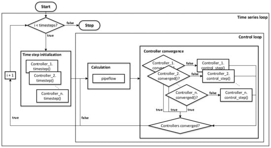
Figure 3.
Flowchart of the time series and controller calculation and how the pipe flow is embedded in the process.
3.2. Illustrating Adaptable MEG Model Setup: Introduction to Pandapipes Multi-Energy
The coupling points of energy infrastructures are facilities such as CHP plants, heat pumps or P2G devices. As their specific models are usually not inherent to a grid calculation, they need to be implemented in a separate structure. In the relevant literature, the concept of energy hubs is prominent in modeling such facilities [56,57]. An energy hub is a generic formulation of a unit that stores or converts energy between different infrastructures. The energy conversion and storage must follow rules which are usually defined by a control scheme.
For this purpose, the multi-energy module of pandapipes extends the controller architecture to couple different grids with the help of special coupling controllers. It defines a superordinate MEG structure containing several grids along multi-energy controllers that can model the energy transfer between them, as shown in Figure 4. For example, a heat pump can be modeled as a unit that converts electrical energy as an input from a power grid into a heat flow as an output to a heat grid. With the help of a heat pump characteristic and the heat grid temperature as second input, an operating point with its coefficient of performance can be calculated. If it is used to control the temperature at the outlet node, several control iterations with successive pipe flow calculations can be necessary to set the power correctly. As the controllers exchange data with the connected grids for the purpose of controlling certain variables, it is easily possible for them to also ensure a correct model of the energy transfer. Thus, they serve as energy hub model implementations as well.
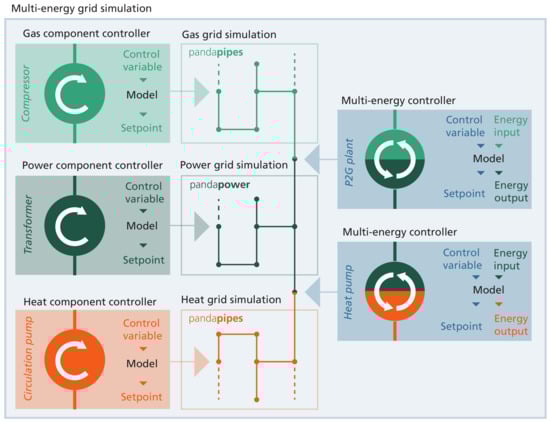
Figure 4.
Overview of the internal structure of the MEG simulation environment based on the pandapipes multi-energy module. It defines a multi-energy grid model consisting of different grids that can be simulated with pandapipes and pandapower functions. These grids are coupled with multi-energy controllers which can vary set points to adjust control variables, as well as model the energy transfer between the coupled grids.
The described approach differs from those used in other MEG simulation tools, as the equations of components in different infrastructures are not summed up in a single system matrix or problem formulation. Therefore, it allows for a high degree of flexibility; nevertheless, it leaves power balance checks to the controller implementations and might lead to a slightly lower performance. Although different calculations for different infrastructures are necessary, such as in an approach using a co-simulation platform, all calculations are performed within the same environment, and no communication interface between different tools is required. This drastically reduces the communication overhead and simplifies the model setup. Moreover, the co-simulation is only performed on the inner structure of the model; a user does not need to learn the specifics of different tools that are plugged together, as pandapipes and pandapower implement an analogous user interface.
In the case of MEG simulations, time series studies are of special interest, as the coupling facilities can be used to shift power peaks in time. Time series simulations also allow analyzing the effectiveness of a certain control scheme. For this purpose, the multi-energy module defines a specialized time series simulation setup for MEGs. In each time step, the controllers of the individual grids are called along with the multi-energy controllers for coupling. Several simulations of each grid might be required until all controllers converge. The multi-energy grid model is the core of the MEG simulation environment based on pandapipes and pandapower. This simulation environment can serve as basis for a framework to tackle challenges in the field of planning and operation analysis of MEGs.
3.3. Illustrating Performance: Comparison between Pandapipes and STANET®
Studies that analyze the operation and design of MEGs usually require a large number of evaluations in different configurations. Furthermore, these studies often require time series simulations as mentioned previously. Therefore, a detailed study of different configurations of an MEG setup can easily require several thousands to millions of single simulation steps, demanding a highly performant core. This requirement can be satisfied by the use of pandapipes. To analyze the performance of pandapipes, we compare it to STANET®, one of the leading piping grid simulation tools available on the German market.
3.3.1. Simulation Setup for the Performance Comparison between Pandapipes and STANET®
As performance comparisons are highly dependent on the given setup, our goal is to create an environment with an equal base for both tools. The following calculations are all run on an ordinary laptop with the specifications given in Table A2 of Appendix B. For the performance comparison, we conduct time series calculations for one entire day in increments of 15 min (96 time steps) for three grids of different sizes. We repeat the calculation 20 times to minimize the effect of outlier results. The following three grids, shown in Appendix C, are analyzed:
- The district heating grid (Figure A1) consists of four heat exchangers and is operated at 6 bar and 43 °C. The demand of each heat exchanger is constant over time. No fluid supply is required, as the grid is considered to be a closed system. Solely the pump ensures a circulation of the fluid and provides the required heat supply.
- The water grid (Figure A2) comprises 105 sinks and is operated at 6 bar as well. To increase the complexity, each sink follows an individual time series.
- The gas grid (Figure A3) is derived from grid data in [7] by removing gas service pipes and aggregating sinks at close-by junctions. It is operated at 1 bar and consists of 1506 sinks, each of which is assigned to one of 132 representative profile types.
The intention of creating three diverse grids is to cover many aspects affecting the performance in an efficient way, while being aware that this approach cannot identify all aspects of simulation performance individually. One of the relevant aspects is the considered energy carrier. For example, simulating a district heating grid in pandapipes always requires a subsequent heat transfer simulation in addition to the hydraulic simulation, as can be seen in the flowchart in Figure 2. This is usually not necessary for simulations of water and gas grids. Therefore, all three simulation options that can be modeled with pandapipes are represented in this work: hydraulic calculation of compressible and incompressible media and the additional heat transfer calculation of incompressible media.
Another aspect that we consider as relevant is the number of different components integrated in a grid model. Therefore, the water grid comprises all components that can be modeled in pandapipes, except for the heat exchanger.
Additionally, the number of nodes and branches has a significant effect on the simulation speed. The three grids were chosen to compare different orders of magnitude of model size, i.e., numbers of nodes and branches.
A last effect we identified is the meshing degree. Therefore, the district heating and water grid have up to 30% higher meshing degrees compared to the gas grid.
We did not investigate the effect of the number of time steps explicitly. However, as each time step is simulated independently, i.e., previous time step results are not used as solver initialization, one can assume that the pure simulation time is increasing linearly with the number of time steps.
An overview of relevant grid characteristics is given in Table 2. It shows that the water grid has the highest number of different component types. The district heating and gas grid contain the same number of component types, but the types differ as well as the model size. The meshing degree of the water grid is slightly higher compared to the district heating grid and much higher compared to the gas grid. The table also shows that the total number of components installed in the different grids increases at a disproportionately low rate, whereas the number of profiles increases at a disproportionately high rate with model size.
Table 2.
Characteristics of the three analyzed grids. Presented are the number of components for each component type, the number of profiles and the meshing degree.
3.3.2. Comparison of Calculation Time
The performance results are displayed in Figure 5, retrieved from 20 simulation runs of 96 time steps for each grid conducted in pandapipes and STANET®, respectively. The average results are represented by the colored bars. The standard deviation is not visualized, as the differences are marginal. The average calculation time and corresponding standard deviation can be found in Table A3 of Appendix D.
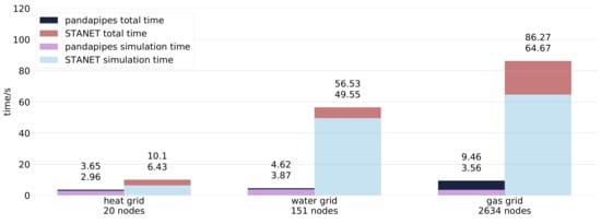
Figure 5.
Calculation time results for three exemplary grids modeled in pandapipes and STANET®. The plots display the average values from 20 simulation runs. A comparison is conducted between the pure simulation time (pipe flow) and the total time, overhead included.
We distinguish between the pure simulation time and the total time. While the simulation time just comprises the required time for the pipe flow calculations, the total time additionally includes the overhead time such as loading profiles and saving results. In each bar plot, the average simulation time is represented by the lower number while the total time by the number above.
For both tools, an increasing model size also leads to an increase of the total simulation time, but with different characteristics. In the case of STANET®, both overhead and pure simulation time increase with the number of nodes and branches. Pandapipes, in contrast, reveals a similar overhead time in the case of the heat and water grid, while it is much bigger for the gas grid simulation. The pure simulation time shows that the solver requires more time for the smaller water grid than for the much bigger gas grid. This anomaly can be led back to the number of solver iterations to reach convergence. While, in the case of the gas grid, usually two to three iterations are required, the solver is called seven to eight times in the case of the water grid. This behavior can probably be explained by the higher meshing degree. As each Newton step of the dependent variables influences more other dependent variables, the number of solver iterations increases for meshed grids. For a closer look at the mathematical model formulation, refer to Appendix A.
A comparison of both tools reveals that pandapipes is always faster than STANET®. While, in the case of the smallest grid, pandapipes is only three times faster, the difference becomes more predominant with model size, making pandapipes up to nine times faster in the case of the gas grid. One reason can be found in the additional overhead such as the graphical user interface (GUI) which STANET® provides.
However, comparing the pure simulation times with one another, the solver alone also claims more time in case of STANET® compared to pandapipes. One of the main reasons we identified might be the readout speed of the profile data. In our examinations, the time spent to read the data from the disc is almost negligible, as we choose a very efficient method. This fact, however, shifts as soon as another data format such as .csv is used, slowing down pandapipes massively. In STANET®, the used format is .dbf, which might cause the big performance difference.
Another reason might be additional implementations in the case of STANET®. For example, it considers the temperature dependency of the dynamic viscosity, which is still neglected in pandapipes. However, the absolute deviations between the pandapipes and STANET® results, visualized in Figure A4 of Appendix E, emphasize that both results still match well.
Furthermore, additional reasons can be causal for the diverging simulation speed, including system dependencies or the investigated grid; both we only analyzed to a limited degree. Furthermore, our look below the hood of STANET® was only possible as far as the manual took us, as the software itself is closed source. Therefore, our conclusions are limited by the information in the instruction book. However, in all our investigations, we tried to be as transparent and unbiased as possible.
4. Solving Problems of Coupled Multi-Energy Grid Simulation with Pandapipes Multi-Energy
4.1. Use Case 1: Local Peak Shaving Strategies to Support the Supply of District Heating Grids
4.1.1. Introduction to the Problem
One of the main reasons for coupling infrastructures on district scale is that the synergies between them can drive energy reduction and reduce overall costs by shifting excess power from one energy carrier to another. This energy shift relies on sophisticated control strategies, which requires time series simulations in the design phase [59].
In the InnoNEX project [60], operation strategies were developed to convert and store available excess power generated by photovoltaic (PV) plants as thermal energy. The excess energy supplied a centrally aligned heat pump connected to a district heating grid, as well as electric heaters installed in the domestic hot water storages of consumer households. In this way, the excess power could be used to cover peak loads occurring at a later time. A detailed model of the district heating grid enabled the evaluation of temperature levels and thus thermal losses in the grid. Nevertheless, no model was created for the electrical grid, which made it impossible to react to certain events such as the overloading of lines. Thus, the state of the electrical network was not respected by the operation strategy.
A similar, but more complex simulation setup, consisting of different tools combined in a co-simulation framework and coupled with an optimization tool, was used in [24,61]. The tools are used to maximize self-consumption from RES and minimize CO2-emissions and electricity imports to the district. Typically, a co-simulation approach acts as a performance bottleneck. This is different with pandapipes multi-energy, where all models are included in one tool, thereby simplifying the model setup.
In the use case we analyze, the heat energy—consisting of the demand for space heating and domestic hot water—for a small neighborhood is supplied by a district heating grid fed by a centrally positioned heat pump. The operation of the heat pump depends on the status of the power grid. Therefore, a coupling model between the electrical and district heating grid has to be provided. We assume that the heat pump has access to a low temperature heat source, so that an inlet temperature of 45 °C or alternatively 55 °C can be supplied. However, legal regulations for legionella require a minimum temperature of the domestic hot water of 55 °C.
Every building connected to the district heating grid has a domestic hot water storage. The storage extracts heat from the heating grid using a heat exchanger. To lift the temperature from the district heating grid temperature level to the required temperature of at least 55 °C, an electric heater is placed inside the storage.
All buildings are equipped with PV plants whose primary purpose is the electrical supply of household appliances. If excess power is available, it can be used by the electric heaters inside the storages. Further excess power is then fed into the electrical distribution grid. Because of their ability to both create and consume power, the households are also called prosumers throughout this use case.
The heat pump heats its storage to 55 °C if the prosumers provide sufficient renewable power to cover the heat pump’s electrical demand. Otherwise, the provided heat pump temperature is 45 °C and the required power is supplied partially by excess PV feed-in and power drawn from the connected distribution grid. As an additional constraint, the temperature of the heat pump can only be raised if this operation mode does not lead to a line overloading in the connected electrical grid. If a line overloading occurs even at a provided temperature of 45 °C, the heat pump enters a power saving mode, where nearly no mass flow is provided and no power is consumed.
The neighborhood consists of 12 buildings. The topologies of the power and district heating grid are shown in Figure 6. A detailed flow chart of the implemented control strategies for the electric heaters and the heat pump can be found in Appendix F.
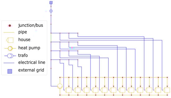
Figure 6.
The power grid (blue) and district heating grid (orange) set up in pandapower and pandapipes, respectively. The power grid also shows an overloaded line highlighted in green color. Besides raising the temperature, the heat pump also provides the functionality of a circulation pump.
4.1.2. Use Case Implementation
Both pandapower and pandapipes only have access to a small set of components, such as sinks and sources. More detailed components, such as the required prosumers and the heat pump, have to be modeled as controllers.
Figure 7 shows a sketch of the prosumer controller and its components. As depicted, each water storage is connected to the pandapipes district heating grid via a heat exchanger. In every time step, the mass flow and inlet temperature (, ) are extracted and used as an input to simulate the water storage temperature. If activated, the electric heater is powered with a constant value of 1 kW. The amount of extracted heat by the water storage heat exchanger and the heat required for space heating is transferred to the pandapipes net ().
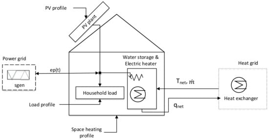
Figure 7.
Sketch of the prosumer and relevant components. Relevant data interfaces are represented by arrows.
Besides, the controller is connected to a static generator (sgen) component in the power grid model. Depending on the sign of the power variable, this component may represent a producer or a consumer. In each time iteration, the current excess power is determined by the prosumer controller according to Equation (1) and transferred to the sgen component. Here, PV(t) denotes the power provided by the PV plant and load(t) denotes the electrical demand of all devices in the household except the electric heater heating the water storage. The latter is described with the variable . If is negative, the available PV power is not sufficient to cover the electrical demand. In this case, power has to be fed in by the power grid.
The described data exchange between the controller and the connected grid models is started via the controller’s time step initialization, where models of arbitrary complexity may be included. The water storage temperature T is computed via the differential Equation (2). A numerical solution for the storage temperature of the next time step is determined using a differential equation solver provided by the Python package scipy [62].
The time series for the PV power plant, the electrical household loads and for space heating are provided as external sources. They have been generated with models described in more detail in [63,64].
A diagram of the implemented heat pump controller and its interfaces to the pandapower and pandapipes components is shown in Figure 8. It is also connected to a water storage. The heat pump feeds directly into the storage (with a provided temperature ), which in turn is connected to the pandapipes district heating grid. The current storage temperature () computed in every time step as well as the mass flow () provided by the pump are parameters for the pandapipes component. The heat pump controller is also connected to a load component of the power grid. It transfers the required power () for operating the heat pump in every time step.
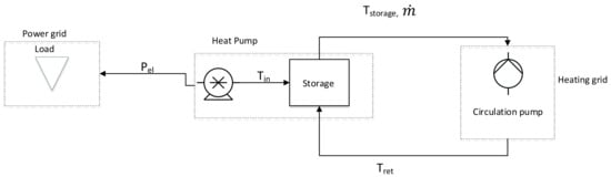
Figure 8.
The heat pump controller component and its connections with the pandapower and pandapipes grid models.
Regarding the district heating grid, it has to be emphasized that transient effects are currently not respected by pandapipes (see also Appendix A). It has to be noted that neglecting inertial effects will lead to a loss of accuracy for the simulation, which can be accepted because of the following reasons:
- The simulation is performed in 15 min increments with the temperature being evaluated every 50 m. The heat pump supplies a pressure which is high enough to make sure that the fluid arrives at the consumers within one time step.
- If inertial effects were not neglected, depending on the ambient temperature and pipe insulation, the fluid temperature would continuously adopt to the steady state. By neglecting inertia, we observe a worst case where the fluid temperature instantaneously mixes with ambient temperature levels. As the primary intention in this use case is to show how the state of one grid influences the state of a coupled grid, this approach is feasible without a detailed analysis of the heating grid.
4.1.3. Result Evaluation
To show that the state of the power grid may influence the state of the district heating grid, we examine two days in July of the selected test reference year 2015 [65]. In this month, the excess power produced by the PV power plants is typically enough to supply not only the electric heaters of the buildings but also the heat pump. Since space heating is hardly required, it is not discussed in the following. On the first day, the green power line depicted in Figure 6 would have been overloaded, so the storage temperature does not rise to 55 °C. This is only possible on Day 2. Figure 9 not only shows the temperature of the heat pump storage, but also a plot for the heat pump control signal. Additionally, the excess power is displayed.
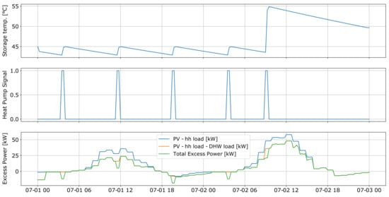
Figure 9.
(Top) The storage temperature of the heat pump storage. (Middle) The Heat Pump control signal. (Bottom) Available excess power for the whole neighborhood. The green line visualizes available excess power after demand for households (hh), domestic hot water (DHW) and heat pump is subtracted.
The blue curve shows the available excess power after the household loads of all houses have been subtracted. The orange line represents the total excess power after the power requirements for the electric heaters are subtracted. The green line shows the amount of total available excess power that could be fed into the external grid. We see that the amount of available excess power is further reduced by the heat pump operation.
A similar result, focused on one building in the neighborhood, is shown in Figure 10. The top panel shows the storage temperature during the two days. The required thermal power is supplied by the district heating grid and the electric heater. The slope of the storage temperature is connected to the demand profile shown in the plot in the middle. The lower panel displays the available excess power for the observed household. Again, the blue curve represents the generated PV output minus the household loads and the orange curve adds the required heater power. Note that the storage temperature plot reflects the control algorithm of Figure A5. For example, the heater is turned off after the secondary set point temperature of 70 °C is reached.
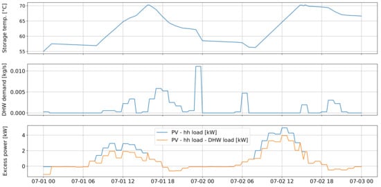
Figure 10.
(Top) The storage temperature of one building in the neighborhood. (Middle) The demand profile for domestic hot water (DHW) for the two observed days. (Bottom) Available excess power for the building. The blue line represents the generated PV output minus the demand of all household (hh) loads except the power needed to heat the drinking water storage. This heater power is considered in the orange line, which represents the total available excess power.
4.2. Use Case 2: Flexibility Provision of Power-To-Gas Devices
4.2.1. State-of-the-Art Review
In some regions of Germany, especially in the north with high shares of wind power, the fluctuating feed-in from RES already leads to grid congestion situations, some of which also occur in distribution grids [66]. One possibility to mitigate such congestion situations is to expand and reinforce the distribution grid, which is a long-term strategy with high capital requirements. Other options include curtailment of renewable feed-in, redispatch with other power plants or demand-side management. Those operational interventions are short-term and the single measures are rather resource sparing. To implement them in a cost-efficient way, market platforms for trading flexibility options have received more attention recently [67]. Sector coupling facilities such as CHP plants or P2G devices are considered to have great potential as such flexibility providers [68,69].
Since local flexibility markets are a rather new concept, the model development is still in its early phase. In [70], CHP plants are modeled with a detailed bidding strategy and some operational limits, but the coupled gas grid and heating infrastructure are neglected completely. In [71], an integrated gas and power grid optimal power flow is presented to use CHP plants with thermal storages as flexibilities for operation cost minimization. The authors showed its performance in a small test case for a two-day period. An analysis of linepack flexibility is presented in [72] with the help of a multi-stage procedure, including several separate evaluations of the gas and power grid. The potential of P2G devices to reduce necessary curtailment of RES is analyzed in [73] with the help of an integrated optimization formulation for the power and gas grid, modeling P2G devices with a constant efficiency.
4.2.2. Use Case Implementation
A model for analyzing flexibility provision was also implemented in pandapower within the project NEW 4.0 [74]. This model is similar to the approach in [75] and will be described in detail in separate publications. An OPF is used to set the active and reactive power values of flexibilities to a cost optimal value which deviates as little as possible from their predefined set points. For P2G devices, a feedback from the coupled grid should be taken into account. There, the P2G devices’ operation could lead to the violation of operational constraints, thus decreasing their potential to serve as flexibilities in the power grid.
An approach to integrate gas grid constraints into the flexibility provision model was developed with pandapipes multi-energy on the basis of synthetically created grids. The medium voltage (MV) electric grid [55,76] geographically overlaps with the medium pressure gas grid [7], as shown in Figure 11 and Figure A6. To better show the effects occurring in the gas grid, we altered some of the data. More details of the two grids are given in Appendix G. The grid data are complemented with time series for load and generation. Standard load profiles are used for electric loads and load profiles based on typical heating demand considering probabilistic occupancy are used for the gas consumers [77,78]. Time series of PV and wind power feed-in are provided for all RES sites and combined into three scenarios: the PV scenario with 100% PV feed-in, the wind scenario with 100% feed-in from wind power and the mix scenario with 50% feed-in from PV and 50% from wind power. Table 3 gives a small summary of the maximum power and annually generated or consumed energy.
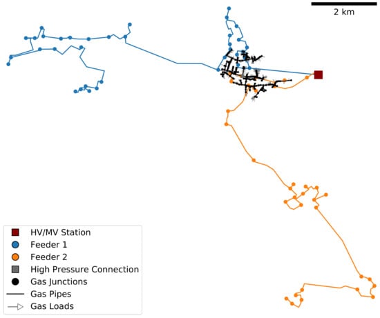
Figure 11.
Structure of the power grid consisting of two feeders and the gas grid that partially overlaps with both feeders.
Table 3.
Maximum power and total energy over year aggregated for the RES in three different scenarios (PV, wind and mix) and for the loads in the power and gas grid.
The operational constraints that lead to adaptations of the RES and P2G feed-in are shown in Table 4, along with boundary conditions. We consider a maximum line current and node voltage in the power grid and a maximum pressure and P2G feed-in in the gas grid. As we analyze two different P2G processes—one with successive methanation and one with direct hydrogen feed-in—there are two different constraints that limit the feed-in. In the configurations with methane feed-in, we assume that there is a uni-directional flow at the reference node, because normally compressors that could feed in gas to the high pressure grid are not part of gas pressure regulation stations. In the configurations with hydrogen feed-in, we assume that the volume fraction at the connected node must remain below 10%.
Table 4.
Constraints and boundary conditions for the grid simulations. Voltage and current limits apply for the whole power grid. Pressure and hydrogen fraction limits apply only for the power-to-gas (P2G) connection node, as the respective maximum value will always occur there. stands for the number of households connected to the gas grid.
We perform a simulation for a full year in increments of 15 minutes with the approach depicted in Figure 12. This approach considers differences in demand and weather occurring over the course of the year. It makes use of the special structure and the time series and controller architecture defined in pandapipes multi-energy. In each time step, constant controllers write values from load and generation profiles to the respective pandapipes and pandapower grid tables. In the case of a single P2G device, one of those values is the maximum P2G power according to the physical correlations described in Appendix H. Based on the results of a subsequent power flow, a central power grid controller checks for constraint violations according to Table 4. In the case of violations, an OPF can reset the power of the P2G devices and RES to comply with the power grid constraints. The next triggered controller is the P2G controller. It first transforms the adapted power of the P2G devices to a mass flow according to a P2G model and performs a pipe flow simulation. Then, it checks for violations of the gas grid constraints. The maximum feed-in constraint can only be violated in the case of multiple installed P2G devices, as otherwise it is pre-calculated as stated above. When it is violated, the possible feed-in is calculated based on the total gas consumption according to the equations described in Appendix H and the necessary mass flow reduction is distributed over all P2G devices proportionally to their identified feed-in. If the maximum pressure constraint is violated, the P2G devices are replaced with reference nodes with fixed pressure at the maximum value to identify the allowed feed-in. After transforming the identified maximum mass flows back to the maximum powers of the P2G devices, they will be considered by the OPF in the next control loop. This feedback from one controller to the other is not a realistic control loop and thus can only be used to identify the technical potential. In reality, these calculations have to be performed with forecasted grid states introducing an uncertainty that needs to be dealt with. We demonstrate that this approach is able to mitigate any constraint violations in Appendix I for an excerpt of a full year simulation shown in Figure A8.
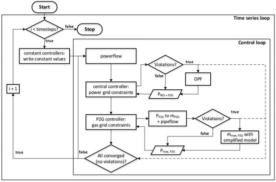
Figure 12.
Setup of the P2G operation for reducing congestions in the power grid. The calculations in pandapower and pandapipes ensure that all power grid and all gas grid constraints are satisfied. For this approach, the pandapipes multi-energy grid structure and its time series and control architecture are used.
4.2.3. Study of the Power-To-Gas Flexibility Potential
As the presented approach ensures a secure operation of both power and gas grid, it can be used to study how P2G devices can effectively be integrated into a coupled infrastructure. We performed a large-scale analysis for different RES scenarios and different numbers, positions and sizes of P2G devices, leading to a total of 462 different configurations. The possible positions of the P2G devices with their connections to power and gas grid are shown in Figure A7. The option of direct hydrogen feed-in is only considered in the case of connection to the reference node. In all other positions, the fluid composition would not be the same everywhere, which is not possible to model with the applied version of pandapipes. An overview of the configuration setup is given in Table 5. We distinguish between the power grid restricted (PR) case, where gas grid constraints are neglected, and the power and gas grid restricted (PGR) case, where gas grid constraints are considered with a feedback loop. More details can be found in Appendix I. Performing such a large study is only possible with the help of a parallelized approach conducted on a computer cluster, as an OPF is very time consuming. Relevant questions that can be addressed with the analysis are to what degree the P2G device can reduce RES curtailment and what influence the gas grid constraints have on this result for different configurations. As the main economic factor in this setting is the curtailed energy, we look at the results of a full year simulation.
Table 5.
Configuration setup analyzed for the P2G flexibility potential study. All combinations lead to a total of 462 different configurations to be analyzed.
For the three RES scenarios, Figure 13 shows results of curtailed energy from RES and the reduction of this curtailment through the P2G devices in relation to the installed P2G capacity (Relative Curtailment Reduction-RCR). The latter is an important key performance indicator, as installation costs of P2G devices mainly scale with the installed capacity. We look at four configurations, one without P2G device, one with the highest RES curtailment reduction, one with the highest impact of the gas grid constraints and one with the highest RCR. As can be seen, the potential to reduce curtailment is especially high in the case of the mix scenario. This is mainly due to the more distributed and lower RES feed-in peaks compared to the PV or wind scenario, which can be absorbed more easily by the P2G devices. The influence of the gas grid constraints is the highest in the PV scenario, which is to be expected, as the highest PV peaks occur during summer, when gas consumption is usually very low and thus the gas feed-in is limited. However, the impact is rather small in general: the P2G potential is reduced by less than 20% in all scenarios for the configurations with the highest curtailment reduction. In the configurations with the highest RCR, this is even less, which raises the question whether a detailed gas grid simulation is necessary in this kind of analysis. It might be possible to identify simple rules that can be considered as constraints in the OPF. Furthermore, it is obvious that position 2 is very promising for placing a P2G device, which is due to its sensitivity to line overloading occurrences in the power grid near that position.
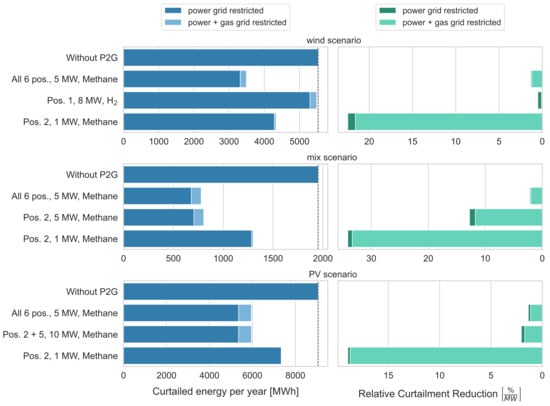
Figure 13.
Analysis of the curtailed RES energy and its relative reduction by the P2G device in relation to the size (right-aligned due to the inverse behavior compared to the curtailment) for the three RES scenarios and different configurations. The simulated cases considering power grid restrictions (PR) and power and gas grid restrictions (PGR) are shown in different colors to highlight the influence of the gas grid constraints on the results. Considering gas grid constraints leads to a lower P2G employment, so that more energy from RES needs to be curtailed.
Another result of interest is how the potential to reduce curtailment changes with the installed capacity and number of P2G devices. Figure 14 shows the RCR for one, two and six installed P2G devices with capacities ranging from 1 to 10 MW in the PGR case. For different positions and RES scenarios, the results vary greatly, as can be seen from the box plots. In general, the curtailment is not reduced much further with increasing P2G capacity, so that the RCR decreases. There are mainly two reasons for this. On the one hand, the higher P2G power is required less often to resolve all congestions due to a lower occurrence of high RES peaks. On the other hand, the higher P2G power is more often restricted by the gas grid constraints. It also means that the RCR is expected to increase with further decreasing P2G size.
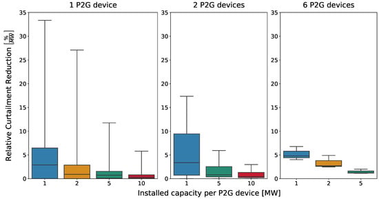
Figure 14.
Influence of the installed capacity and number of P2G devices. For the configurations with devices at one, two and six positions, the relative reduction of renewable energy sources (RES) curtailment is given as distribution over all analyzed configurations.
The previous analysis is of qualitative nature and it is not possible to derive the optimal P2G capacity from it. There are many unconsidered factors, besides the RCR, that influence whether a P2G device can be operated economically. The costs of installing and operating a P2G device need to be compared to RES curtailment costs and grid expansion costs. Furthermore, there might be other business cases for the P2G device. Thus, it is necessary to compare different options, such as operating the device at times of low electricity prices, implementing a local flexibility market or direct contracting for delivering ancillary services. These options could even complement each other. Analyzing these questions would require an extension of the methods we presented.
5. Summary and Conclusions
We present the new open source simulation tool pandapipes. When coupled with pandapower through the multi-energy module, it forms a powerful environment for the coupled simulation of MEGs. To the best of our knowledge, it is the first such simulation environment that is available open-source and does not require proprietary software to work. After analyzing the field of MEG simulation approaches and tools, we defined three criteria that should be addressed by a dedicated tool: clear data structure, adaptable MEG model setup and performance. In the following, we describe the internal structure and performance of pandapipes in relation to these criteria. Then, we demonstrate two use cases. In the first, we analyzed local peak shaving strategies in combination with district heating grids. In the second case, we performed a large study on the potential of a P2G device to serve as flexibility in a coupled power and gas grid. Although these use cases are based on artificial data, they are examples of typical research studies and show that the presented tool is very powerful at performing coupled simulations. They also underline the importance of the criteria with respect to large research studies.
We explain that new holistic planning approaches require tools which are able to model the effects of interactions between different infrastructures. Such tools must implement detailed models of different grids and their interconnections and handle large amounts of data efficiently. The open source tool pandapipes is such a tool, as it addresses the criteria that we specify above:
- With its internal architecture, pandapipes addresses the criterion of a clear data structure. Using pandas tables for input parameters and results enables an easy setup and adaptation of grid states and post-processing with the help of convenient pandas functions. Large time series simulations can be performed and results stored efficiently. The use of numpy arrays with a unified design makes the internal structure clear for developers, and parts of the calculation logic can be adapted without putting much effort into its restructuring.
- The specialized multi-energy module addresses the criterion of an adaptable MEG model setup. Models for coupling components can be chosen from the existing implementations or defined by the user himself. In the use cases, we showed the flexibility of these models, as controllers were defined for heat pumps and P2G devices that relied on results of heating and gas grid simulations. This information can be exchanged at run time of the control loop. By connecting different control strategies and types of simulations, a wide range of research questions can be addressed.
- The comparison to STANET® illustrated the performance of pandapipes, which we identified as another criterion. Comparing run times of time series simulations for different grid models between the two tools revealed that pandapipes is faster in each simulation setup. One possible reason is the handling of time series data, which is especially important in MEG simulations. The performant core makes pandapipes a perfect tool for extensive investigations, including probabilistic grid planning, time series, Monte Carlo and placement studies. Unlike with co-simulation environments, the coupling of simulations hardly adds any overhead to the simulation time. The demonstrated use cases underline how crucial performance is, as a large number of simulations had to be performed for each of the studies. Comparisons to other tools, especially open source tools such as EPANET [79], should be considered in the future.
One of the main findings in the demonstrated use cases is that the coupling components between different grids are important influencing factors for the grid states. A typical use case for sector coupling is to shift excess power from electric grids to other energy carriers, such as heat or gas. In the first use case, the operation strategy of a central heat pump connected to a district heating grid is influenced by the possible event of overloaded lines in the power grid. This operation strategy in turn influences the heat supplied to the district heating grid consumers and necessitates the use of additional decentralized heaters. In the second use case, P2G devices are used to reduce voltage and line loading in a power grid by feeding hydrogen or methane into a natural gas grid. The feed-in has to be limited in some cases due to operational limits of pressure, hydrogen blending or gas consumption. Many of the effects occurring in both use cases can only be quantified with the help of detailed power, gas and district heating grid simulations. This is possible with pandapipes for steady-state simulations, which are often precise enough in the planning phase and for the simulation of long periods.
In the Introduction, we give a short overview of challenges in the field of energy infrastructure design, which pandapipes can help to address. The assessment of supply options with different energy infrastructures can be performed with pandapipes but requires detailed scenarios as input and information of costs for further analysis. Grid integration and expansion studies have been performed with pandapower already, and with pandapipes the principles can be transferred to district heating, gas or hydrogen grids as well, also considering interconnections. The analysis and optimization of operation strategies was demonstrated in the use cases, where the performance of pandapipes and the possibility to perform the analysis on multiple cores was crucial. In the case of urban planning, detailed modeling is especially important for new districts due to the small extent of the analyzed infrastructure. Algorithms in analogy to [52] can be transferred to pandapipes and used as planning approaches. The analysis of market design in some cases also necessitates a detailed view of the regulated grid infrastructure. An approach implemented with the help of pandapower in [70] could make use of pandapipes as well in order to simulate sector coupling effects. In research, open source tools are gaining attention, as they allow collaboration, model adaptation for specific use cases and large-scale parallel utilization. Furthermore, open source tools are inherently transparent with respect to the model implementations, which is especially important for reproducibility.
Although the presented simulation environment covers a large variety of use cases, there are still model limitations that shall be addressed in future releases of pandapipes. For instance, up to now, the heat transfer option is restricted to incompressible fluids, because in pandapipes the calculated temperature does not influence the hydraulic fluid properties such as density or viscosity. Transient calculations can be decisive in modeling effects of heat propagation in heat grids with integrated storages, but also for modeling gas transport grids. Another missing feature is the calculation of fluid mixtures and their propagation in a piping grid, especially for the evaluation of blending hydrogen into natural gas grids. The models could be based on the descriptions in [80].
Other extensions could increase the range of functions and the performance in order to make pandapipes more attractive for specific use cases. They include a speed-up of time series simulations, new or extended libraries for component models and controllers, topology analyses and grids for testing purpose. With the increasing interdependency of infrastructures, an integration of power and piping grid simulations on kernel level will also become more important. This is especially true for OPF calculations, where an optimal operation strategy must comply with the constraints of all integrated grids. With such an integrated OPF, the flexibility provision model could be extended so that the optimization is performed in one step without feedback loop. For this purpose, an approach similar to those of Geidl and Andersson [12] or Acha et al. [71] could be chosen, or a port to existing tools could be used, such as the GasPowerModels Julia package [81].
Author Contributions
Conceptualization, T.M.K., D.L., D.C. and S.R.D.; data curation, D.L., D.C. and S.R.D.; formal analysis, D.L., D.C. and S.R.D.; funding acquisition, T.M.K. and M.B.; investigation, D.L., D.C. and S.R.D.; methodology, D.L., D.C. and S.R.D.; project administration, T.M.K.; resources, T.M.K. and M.B.; software, D.L., D.C. and S.R.D.; supervision, T.M.K. and M.B.; validation, D.L., D.C. and S.R.D.; visualization, D.L., D.C. and S.R.D.; writing—original draft, D.L., D.C. and S.R.D.; and writing—review and editing, T.M.K. and M.B. All authors have read and agreed to the published version of the manuscript.
Funding
This research was funded by the Federal Ministry for Economic Affairs and Energy (BMWi) within the research projects “NEW 4.0” (Grant No. 03SIN411), “InnoNEX” (Grant No. 03EGB0009G) and “INTEEVER II” (Grant No. 03ET4069C), based on a decision of the Parliament of the Federal Republic of Germany. The authors take full responsibility for the content of this work.
Acknowledgments
The authors thank Christian Spalthoff (Fraunhofer IEE) for his design and illustration support.
Conflicts of Interest
The authors declare no conflict of interest.
Abbreviations
The following symbols and abbreviations are used in this manuscript:
| Symbols | Explanation | Unit |
| A | area | m2 |
| heat capacity | ||
| d | pipe diameter | m |
| h | height | m |
| H | heating value | |
| I | current | A |
| l | pipe length coordinate | m |
| mass flow | ||
| N | number | [-] |
| p | pressure | Pa |
| pressure difference | Pa | |
| P | active power | W |
| q | heat flow | |
| T | temperature | K |
| v | flow velocity | |
| V | voltage | V |
| x | fraction | 1 |
| heat transfer coefficient | ||
| pressure loss coefficient | 1 | |
| efficiency | [-] | |
| Darcy friction factor | 1 | |
| fluid density | ||
| Subscripts | ||
| b | referring to a branch | |
| methane | ||
| external | ||
| hydrogen | ||
| households | ||
| maximum | ||
| n | referring to a node | |
| referring to node 1 (entering a branch) | ||
| referring to node 2 (leaving a branch) | ||
| N | referring to the reference state | |
| natural gas | ||
| referring to the network | ||
| power-to-gas device | ||
| at reference node | ||
| s | superior | |
| thermal | ||
| at slack node | ||
| referring to the surface | ||
| volumetric | ||
| Abbreviations | ||
| CHP | Combined heat and power | |
| ESMO | Energy system modeling and optimization | |
| GUI | Graphical user interface | |
| GS | Grid simulation | |
| MEG | Multi-energy grid | |
| MES | Multi-energy system | |
| MV | Medium voltage | |
| OPF | Optimal power flow | |
| P2G | Power-to-gas | |
| PGR | Power and gas grid restricted | |
| PR | Power grid restricted | |
| PV | Photovoltaic | |
| RCR | Relative curtailment reduction | |
| RES | Renewable energy sources | |
| sgen | static generator |
Appendix A. Mathematical Model Formulation in Pandapipes
For any piping grid, the laws of Kirchhoff apply. The nodal rule is given by Equations (A1) and (A2), stating that incoming and outgoing mass and energy flows of a node must balance out. Here, denotes the mass flow of a branch connected to the node and denotes the mass flow that enters or leaves the system through the node itself. is the heat flow entering or leaving a node and is the number of branches connected; the subscripts in and out denote incoming and outgoing flows. As a perfect mixture is assumed at each node, the temperature of all outgoing flows equate to the node temperature. Equation (A2) also assumes that no mass or energy enters or leaves the system through the node.
The mesh rule, given by Equations (A3) and (A4), states that pressure or temperature differences within a mesh must sum up to 0. Here, denotes the number of branches that span up one mesh.
To solve for the unknown variables of node pressures and branch velocities, equations describing dependencies of these variables must be set up. Physical models are implemented for different components in pandapipes, which are divided into three types, namely nodes, branches connecting two nodes and node elements, which are connected to single nodes and change their properties. Since the component models are implemented as classes, they can be extended by anyone, if the desired component behavior is not represented by the existing components. The following component models are implemented in pandapipes:
- Junctions are the node representations. Their model implementation corresponds to the mass and energy flow balance as formulated in Equations (A1) and (A2). However, since there are only formulations for pressure and temperature drops in the system of equations, for at least one junction, the pressure and temperature need to be preset as boundary conditions.
- External grids represent connections to other systems. This node element fixes pressure or temperature for the connected junction to form the above stated boundary condition, thus turning it into a reference node.
- Sinks and sources are node elements which insert a mass flow entering or leaving the connected junction.
- Pipes are the main branch components, i.e., they connect two junctions, respectively. Their physical representation is explained in the following paragraphs.
- Valves are branch components that can also disconnect the two connected junctions from each other, depending on an “opened” flag. They are modeled as branches with length 0, but can still introduce a lumped pressure loss.
- Pumps are branch components that introduce a pressure lift. The pressure lift is calculated according to a characteristic that sets the operating point in dependency of the calculated flow rate.
- Circulation pumps are useful for district heating grid calculations. At the outgoing junction, the pressure is fixed and at the incoming junction the mass flow is set. This behavior corresponds to two node elements: an external grid and a sink. It is a simplified component neglecting operation limitations of a real pump.
An overview of the existing component models with the respective input parameters and results is given in Table A1 and additional information can be found in the documentation [82]. Further component models, e.g., for compressors or pressure controllers, are currently under development. In the following, we explain the equations introduced for branch components. The presented equations correspond to the pipe component model, however they are applicable to other branch components as well, considering their respective characteristics. For example, valves have a length of 0, which means that the Darcy friction term is neglected and only a lumped pressure loss is introduced.
Table A1.
Input parameters and results for the different pandapipes components.
Table A1.
Input parameters and results for the different pandapipes components.
| Component | Input Parameters | Results | ||||
|---|---|---|---|---|---|---|
| Name | Description | Unit | Name | Description | Unit | |
| Junction | rated pressure | bar | p | pressure | bar | |
| initial temperature | K | T | temperature | K | ||
| h | height | m | ||||
| External grid | fixed pressure | bar | mass flow to grid | |||
| fixed temperature | K | |||||
| Sink/Source | set mass flow | mass flow to / from node | ||||
| C | scaling factor | - | ||||
| Pipe | l | length | km | mean velocity | ||
| d | diameter | m | pressure difference | bar | ||
| k | roughness | mm | temperature at junction 1 | K | ||
| loss coefficient | - | temperature at junction 2 | K | |||
| heat transfer coefficient | mass flow through pipe | |||||
| external heat flow | W | norm volume flow | ||||
| external temperature | K | Re | Reynolds number | - | ||
| s | number of sections | - | Darcy friction factor | - | ||
| Valve | d | diameter | m | mean velocity | ||
| flag for flow | - | pressure difference | bar | |||
| loss coefficient | - | mass flow through valve | ||||
| norm volume flow | ||||||
| Pump | pump standard type (for characteristic) | - | pressure difference | bar | ||
| Circulation Pump | pressure set point | bar | pressure difference | bar | ||
| pressure lift | bar | mass flow through pump | ||||
| temperature set point | K | |||||
For an incompressible medium, the pressure variation along a pipe section with length can be described using Equation (A5). The pressure difference is caused by three effects, described with the terms on the right-hand side of the equation: the pressure loss due to friction is proportional to the Darcy friction factor . It also depends on the pipe diameter d.
A lumped pressure loss can be expressed using the pressure loss coefficient . This pressure loss is introduced, e.g., by bends or components which are not represented by a component model. The pressure losses due to both friction and lumped components are proportional to the dynamic pressure , where is the fluid density and v is the flow velocity.
A pressure difference introduced by a given height difference between the connected junctions is given by the last term. This difference depends on the fluid density and the gravitational acceleration g.
In the case of compressible media, the density of the medium is expressed by using the ideal gas law and a reference state, as shown in Equation (A7).
The reference state, noted with the index N, corresponds to the known gas normal properties. To add real gas behavior, the equations resulting from the description as an ideal gas can be modified by a compressibility factor. For the reference state, a velocity can be found with the help of relation (A8) for the mass flow inside the pipe. By inserting Equation (A7), the system velocity can be formulated as a function of the velocity of the reference state (Equation (A9)).
Inserting Equation (A9) into Equation (A5) leads to Equation (A10) (including only pressure losses due to pipe friction).
Thus, the pressure losses in the pipe can be determined for the completely known reference state. Because this equation only contains the gas velocity with respect to the reference state , the gas velocity for the system has to be determined after the calculation of pressure losses from Equation (A9).
Compressible media lead to a continuous velocity and pressure distribution along a pipe. To capture these distributions, derivatives with respect to the pipe coordinate of Equation (A10) are described with the finite difference method. As a result, the user can divide a pipe into several subsections, gaining a finer resolution of solution variables for the pipe of interest.
If the heat transfer mode is started, Equation (A11) is solved for a pipe section with length . The right-hand side describes a heat flow exchanged with the ambient, which has a temperature of . This exchange is described via the heat transfer coefficient . Besides, an optional heat flow can be defined, which is evenly distributed along the pipe length. To solve this equation, the mass flow has to be known. It can be determined by a preceding hydraulic calculation. The solution of Equation (A11) again requires a finite difference method. As the equation does not contain a partial derivative with respect to time, temperature distributions do not include inertial effects.
In pandapipes, the described equations are set up in a system of nonlinear equations and the unknown variables are found with the help of a Newton–Raphson method. We shortly describe the procedure to find hydraulic unknown variables for nodes and for branches in the following. Starting with an initial guess, the derivatives of the node and branch equations for the unknown variables at the current guess are determined to find the next Newton step according to Equation (A12) for nodes and Equation (A13) for branches. Here, , and denote the Newton step to be found for the branch velocities and the respective pressures of the two nodes connected to each branch. denotes the pressure drop along the branch and the mass flow through the branch. For these expressions, Equations (A5) and (A8) need to be inserted. These equations span a linearized system of equations that is solved for in pandapipes using the sparse matrix solver of scipy, which is based on LU factorization [83].
Appendix B. System Specification of the Laptop Used for the Performance Comparison between Pandapipes and STANET®
Table A2.
PC setup for the performance test between pandapipes and STANET®.
Table A2.
PC setup for the performance test between pandapipes and STANET®.
| Operating System | Microsoft Windows 10 (64 bit) |
|---|---|
| CPU | Intel Core i7-6700HQ |
| system memory | 16 GB |
| solid-state drive | Samsung MZ7TY256HDHP-000L7 |
| graphic cards | Intel HD Graphics 530, NVIDIA GeForce 940MX |
Appendix C. Plots Displaying Grids Used for Performance Comparison

Figure A1.
Heat grid used for performance comparison. It comprises 20 junctions and 18 pipes, supplies 4 heat exchangers and is operated at 6 bar and 43 ℃.
Figure A1.
Heat grid used for performance comparison. It comprises 20 junctions and 18 pipes, supplies 4 heat exchangers and is operated at 6 bar and 43 ℃.


Figure A2.
Water grid used for performance comparison. It comprises 151 junctions and 149 pipes, supplies 105 sinks and is operated at 6 bar.
Figure A2.
Water grid used for performance comparison. It comprises 151 junctions and 149 pipes, supplies 105 sinks and is operated at 6 bar.


Figure A3.
Reduced gas grid used for performance comparison. It comprises 1128 junctions and 1128 pipes, supplies 1506 sinks and is operated at 1 bar.
Figure A3.
Reduced gas grid used for performance comparison. It comprises 1128 junctions and 1128 pipes, supplies 1506 sinks and is operated at 1 bar.

Appendix D. Calculation Results of Performance Comparison between Pandapipes and STANET®
Table A3.
Results of the performance comparison: Average calculation time with standard deviation for the three compared grids.
Table A3.
Results of the performance comparison: Average calculation time with standard deviation for the three compared grids.
| Heat Grid | Water Grid | Gas Grid | |||
|---|---|---|---|---|---|
| total time | pandapipes | mean [s] standard deviation [s] | 3.65 | 4.62 | 9.46 |
| STANET® | mean [s] standard deviation [s] | 10.1 | 56.53 | 86.27 | |
| simulation time | pandapipes | mean [s] standard deviation [s] | 2.96 | 3.87 | 3.56 |
| STANET® | mean [s] standard deviation [s] | 6.43 | 49.55 | 64.67 | |
Appendix E. Deviation between Pandapipes and STANET® Results
Table A4 shows the calculation results for the three compared grids in pandapipes and STANET®. To avoid division by near zero values, we compare the average results and their mean deviations for pressure, velocity and temperature (only heat grid). The spread of absolute deviations is also shown in Figure A4.
Table A4.
Comparing the average junction and pipe results with the average deviation.
Table A4.
Comparing the average junction and pipe results with the average deviation.
| Measurand in the Corresponding Grid | Average Result | Mean Deviation | Relative Deviation | |
|---|---|---|---|---|
| pressure [bar] | heat grid | 6.00 | 0.00065 | 0.011% |
| water grid | 5.96 | 0.00015 | 0.0025% | |
| gas grid | 0.94 | 2.41 × | 0.0025% | |
| velocity | heat grid | 0.015 | 3.76 × | 0.25% |
| water grid | 0.0049 | 0.00027 | 5.42% | |
| gas grid | 1.45 | 0.0010 | 0.071% | |
| temperature [℃] | heat grid | 47.31 | 0.42 | 0.89% |

Figure A4.
Absolute deviations of the pandapipes compared to the STANET® results. From left to right, one can see the absolute deviations of pressure at the junctions, fluid velocity in the pipes and temperature at the junctions for each grid, respectively. The absolute temperature deviation is only displayed for the heat grid, as it is the only one where this value is derived from a heat transfer calculation.

Appendix F. Use Case 1: Additional Information on the Peak Shaving Algorithm
This section provides some additional information about the heat pump and prosumer controller. The control strategies implemented for the heater components and the heat pump are shown in Figure A5.

Figure A5.
Implemented control algorithms for the electric heaters inside the households (left) and the central heat pump (right).
Figure A5.
Implemented control algorithms for the electric heaters inside the households (left) and the central heat pump (right).

Both algorithms introduce two set points, a primary (T_set_pr) and a secondary (T_set_sec), to control temperature values inside the connected storages. The left side illustrates the control for the electric heaters. If the storage temperature lies above the secondary set point, the heater is switched off, because the maximum temperature of the storage is exceeded. Otherwise, the algorithm checks if there is enough excess power provided by the PV plant to switch on the heater. If this is not the case, the heater is still switched on if the temperature is below the primary set point minus an offset of 2.5 K. In this case, the necessary power is provided by the power grid. Provided that there is still not enough excess power available, the heater is switched off if the storage temperature is above the primary set point plus an offset of 2.5 K. If the temperature is between the offsets, the current state of the heater remains unchanged. This introduces a hysteresis in order to avoid a rapid change of state of the heater.
The control algorithm of the heat pump works in a comparable way. The most important difference is that the algorithm checks for a line overloading if excess power is available.
Appendix G. Use Case 2: Details of the Analyzed Grids
The analyzed power grid is the northern part of the generic MV Oberrhein grid that is openly available in pandapower [55]. In this part of the grid, a primary substation supplies two feeders with a total of 62 secondary substations and 4 directly connected MV loads. At 61 nodes, PV plants are installed, most of which can be allocated in connected low voltage grids. These generators are scaled and modeled as PV plants and partially as wind power plants in the P2G use case. The connected gas grid is a distribution grid that directly supplies a total of 1506 household loads through pipelines operated at medium pressure (around 700 mbar). Pressure regulators reduce the pressure at the household connection point to meet the required pressure of 20–25 mbar. The grid is a tree-type network without rings in its structure. Since the extension of the grid is relatively small compared to typical gas distribution grids, the lengths of all pipes were scaled up to show effects in the change of pressure when installing a P2G device. This adaption would alter the true geographic coordinates, but since the case study is only theoretical, the geographic changes of the overlapping grids can be neglected. Furthermore, the high pressure grid connection was shifted, the overall pressure level was lowered and the pipe roughness slightly increased compared to the original data [7]. All the changes do not affect the validity of the results or their transferability. A detailed view of the gas grid with its overlap of the power grid in the initial form is shown in Figure A6.

Figure A6.
Overlapping area of the gas and power grid used for the analysis of flexibility provision.
Figure A6.
Overlapping area of the gas and power grid used for the analysis of flexibility provision.

The positions of the P2G devices that were considered in the case study are shown in Figure A7.

Figure A7.
Overview of the gas grid and possible connections of the P2G devices in the power and gas grid respectively.
Figure A7.
Overview of the gas grid and possible connections of the P2G devices in the power and gas grid respectively.

Appendix H. Use Case 2: Implementation of the Feed-In Restriction
The feed-in of the P2G devices is restricted by a proportional value of the consumed gas. In the case of a single P2G device, this value can be calculated prior to the OPF calculation in order to save simulation effort. This also means that, in the case of hydrogen feed-in, no additional pipe flow calculation has to be performed to analyze constraint violations, as the maximum pressure restriction cannot be violated at the reference node. In the case of methane feed-in at a single node, the maximum P2G power can be calculated with Equation (A14). Here, denotes the mass-related higher heating value of methane and the P2G efficiency with included methanation, which is set to 54 %. In this formulation, the properties of the fed-in methane are assumed to be the same as for the replaced natural gas.
In the case of direct hydrogen feed-in, some more considerations have to be taken into account due to blending. On the one hand, the energy content of the mixed fluid must equal the energy content of the natural gas transported without blending. This correlation is given in Equation (A15), in which the subscript refers to the transported natural gas and to hydrogen. In the use case, the natural gas is a mixture of high calorific gases (H-Gas), which is typical of German gas grids. Using the higher calorific value is a simplification, as usually the required energy content depends on the type of burners installed in the connected households, which is unknown in the case study. The P2G efficiency without methanation is set to 61 %. The required P2G power to reach a certain hydrogen mass flow is described by Equation (A16). With the given volume fraction of hydrogen and the relation between volume and mass flow via the respective density, the mass flows of hydrogen and natural gas at the feed-in point can be described by Equation (A17).
Appendix I. Use Case 2: Results for Ten Exemplary Hours
To demonstrate how the control loop of the coupled simulation works, we analyze the results of a configuration with a P2G device of 10 MW installed capacity at position 4 and included methanation. Figure A8 shows important simulation results in the power and gas grid for ten exemplary hours. We compare three different cases. The base case, which does not include any optimization or RES curtailment, thus leading to constraint violations in the power grid. The power grid restricted (PR) case includes RES curtailment and a P2G operation with the help of an OPF, but no feedback from the gas grid. Constraint violations in the gas grid might occur, as the P2G operation only follows the requirements of the power grid. The power and gas grid restricted (PGR) case also considers the gas grid constraints and the P2G power is reduced in case of violations, leading to a higher curtailment of RES plants. The left panels of Figure A8 show the results of the power grid. The RES feed-in has to be reduced drastically in most time steps in order to comply with the power grid constraints. Otherwise, line loading and voltage exceed the limits by far. On the right, results of the gas grid are displayed. Here, the feed-in from the P2G device has to be reduced in some time steps in order to comply with the gas grid constraints. The mass flow at the reference that represents the feed-in from the high pressure gas grid would in some time steps become negative. This does not comply with the uni-directional flow constraint. In some time steps, the maximum pressure at the connected gas grid node would also be exceeded. Only in the PGR case all constraints are satisfied at all times, which cannot be guaranteed in the PR or base case.

Figure A8.
Time series over 10 h selected from one P2G study configuration. We compare three cases: the base case (index base) without flexibility provision; the power grid restricted case (index PR) with flexibility provision neglecting gas grid constraints; and the power and gas grid restricted case (index PGR) with flexibility provision and gas grid controller. All constraints are marked with a black dashed line. (a) Total power from RES; (b) maximum line loading at any line in the power grid; (c) maximum voltage at any node in the power grid; (d) mass flow feed-in from the P2G device into the gas grid; (e) mass flow feed-in by the gas reference node; and (f) maximum pressure at any node in the gas grid.

References
- European Commission. The European Green Deal Sets Out How to Make Europe the First Climate-Neutral Continent by 2050, Boosting the Economy, Improving People’s Health and Quality of Life, Caring for Nature, and Leaving no One Behind. Available online: https://ec.europa.eu/commission/presscorner/detail/en/IP_19_6691 (accessed on 11 August 2020).
- European Commission. Communication from the Commission to the European Parliament, the Council, the European Economic and Social Committee and the Committee of the Regions: Powering a climate-neutral Economy: An EU Strategy for Energy System Integration. Available online: https://ec.europa.eu/energy/sites/ener/files/energy_system_integration_strategy_.pdf (accessed on 11 August 2020).
- European Commission. Communication from the Commission to the European Parliament, the Council, the European Economic and Social Committee and the Committee of the Regions: A Hydrogen Strategy for a Climate-Neutral Europe. Available online: https://ec.europa.eu/energy/sites/ener/files/hydrogen_strategy.pdf (accessed on 11 August 2020).
- Mancarella, P.; Andersson, G.; Pecas-Lopes, J.A.; Bell, K. Modelling of integrated multi-energy systems: Drivers, requirements, and opportunities. In Proceedings of the 19th Power Systems Computation Conference (PSCC), Genoa, Italy, 20–24 June 2016; IEEE: Piscataway, NJ, USA, 2016; pp. 1–22. [Google Scholar] [CrossRef]
- Then, D.; Spalthoff, C.; Bauer, J.; Kneiske, T.M.; Braun, M. Impact of Natural Gas Distribution Network Structure and Operator Strategies on Grid Economy in Face of Decreasing Demand. Energies 2020, 13, 664. [Google Scholar] [CrossRef]
- Then, D.; Hein, P.; Kneiske, T.M.; Braun, M. Analysis of Dependencies between Gas and Electricity Distribution Grid Planning and Building Energy Retrofit Decisions. Sustainability 2020, 12, 5315. [Google Scholar] [CrossRef]
- Kisse, J.M.; Braun, M.; Letzgus, S.; Kneiske, T.M. A GIS-Based Planning Approach for Urban Power and Natural Gas Distribution Grids with Different Heat Pump Scenarios. Energies 2020, 13, 4052. [Google Scholar] [CrossRef]
- Dall’Anese, E.; Mancarella, P.; Monti, A. Unlocking Flexibility: Integrated Optimization and Control of Multienergy Systems. IEEE Power Energy Mag. 2017, 15, 43–52. [Google Scholar] [CrossRef]
- Braun, M.; Krybus, I.; Becker, H.; Bolgaryn, R.; Dasenbrock, J.; Gauglitz, P.; Horst, D.; Pape, C.; Scheidler, A.; Ulffers, J. Verteilnetzstudie Hessen 2024–2034: Studie im Auftrag des Hessischen Ministeriums für Wirtschaft, Energie, Verkehr und Landesentwicklung: Abschlussbericht. Available online: https://www.energieland.hessen.de/verteilnetzstudie_hessen (accessed on 13 August 2020).
- Scheidler, A.; Bolgaryn, R.; Ulffers, J.; Dasenbrock, J.; Horst, D.; Gauglitz, P.; Pape, C.; Becker, H. DER Integration Study for the German State of Hesse–Methodology and Key Results. In Proceedings of the 25th International Conference on Electricity Distribution (CIRED 2019), Madrid, Spain, 3–6 June 2019. [Google Scholar]
- Liu, Y.; Gao, S.; Zhao, X.; Zhang, C.; Zhang, N. Coordinated Operation and Control of Combined Electricity and Natural Gas Systems with Thermal Storage. Energies 2017, 10, 917. [Google Scholar] [CrossRef]
- Geidl, M.; Andersson, G. Optimal Power Flow of Multiple Energy Carriers. IEEE Trans. Power Syst. 2007, 22, 145–155. [Google Scholar] [CrossRef]
- Then, D.; Loskarn, S.; Kaiser, J.; von Appen, J.; Kneiske, T.; Buchholz, S.; Stockinger, V.; Muender, M.; Schuetz, A. Development of an electricity, heat and mobility concept at district level under consideration of sector coupling for the Lagarde Campus Bamberg. In Proceedings of the ETG Symposium on International ETG-Congress 2019, Esslingen, Germany, 8–9 May 2019; pp. 1–6. [Google Scholar]
- Asarpota, K.; Nadin, V. Energy Strategies, the Urban Dimension, and Spatial Planning. Energies 2020, 13, 3642. [Google Scholar] [CrossRef]
- Caramizaru, A.; Uihlein, A. Energy Communities: An Overview of Energy and Social Innovation; EUR; Publications Office of the European Union: Luxembourg, 2020; Volume 30083. [Google Scholar]
- Cesena, E.A.M.; Loukarakis, E.; Good, N.; Mancarella, P. Integrated Electricity-Heat-Gas Systems: Techno-Economic Modeling, Optimization, and Application to Multienergy Districts. Proc. IEEE 2020, 1–19. [Google Scholar] [CrossRef]
- Mancarella, P.; Chicco, G.; Capuder, T. Arbitrage opportunities for distributed multi-energy systems in providing power system ancillary services. Energy 2018, 161, 381–395. [Google Scholar] [CrossRef]
- Mengelkamp, E.; Diesing, J.; Weinhardt, C. Tracing local energy markets: A literature review. It Inf. Technol. 2019, 61, 101–110. [Google Scholar] [CrossRef]
- Chertkov, M.; Andersson, G. Multienergy Systems. Proc. IEEE 2020, 108, 1387–1391. [Google Scholar] [CrossRef]
- Thurner, L.; Scheidler, A.; Schäfer, F.; Menke, J.H.; Dollichon, J.; Meier, F.; Meinecke, S.; Braun, M. Pandapower—An Open-Source Python Tool for Convenient Modeling, Analysis, and Optimization of Electric Power Systems. IEEE Trans. Power Syst. 2018, 33, 6510–6521. [Google Scholar] [CrossRef]
- Hagberg, A.A.; Schult, D.A.; Swart, P.J. Exploring Network Structure, Dynamics, and Function using NetworkX. In Proceedings of the 7th Python in Science Conference, Pasadena, CA, USA, 19–24 August 2008; pp. 11–15. [Google Scholar]
- Hunter, J.D. Matplotlib: A 2D Graphics Environment. Comput. Sci. Eng. 2007, 9, 90–95. [Google Scholar] [CrossRef]
- Jordahl, K.; van den Bossche, J.; Wasserman, J.; McBride, J.; Fleischmann, M.; Gerard, J.; Tratner, J.; Perry, M.; Farmer, C.; Hjelle, G.A.; et al. Geopandas/Geopandas: v0.7.0. Zenodo 2020. [Google Scholar] [CrossRef]
- Widl, E.; Leitner, B.; Basciotti, D.; Henein, S.; Ferhatbegovic, T.; Hofmann, R. Combined Optimal Design and Control of Hybrid Thermal-Electrical Distribution Grids Using Co-Simulation. Energies 2020, 13, 1945. [Google Scholar] [CrossRef]
- Drauz, S.R.; Spalthoff, C.; Würtenberg, M.; Kneikse, T.M.; Braun, M. A modular approach for co-simulations of integrated multi-energy systems: Coupling multi-energy grids in existing environments of grid planning & operation tools. In Proceedings of the 2018 Workshop on Modeling and Simulation of Cyber-Physical Energy Systems (MSCPES), Porto, Portugal, 10 April 2018; IEEE: Piscataway, NJ, USA, 2018; pp. 1–6. [Google Scholar] [CrossRef]
- Ruf, J.; Zimmerlin, M.; Sauter, P.S.; Koppel, W.; Suriyah, M.R.; Kluwe, M.; Hohmann, S.; Leibfried, T.; Kolb, T. Simulation Framework for Multi-Carrier Energy Systems with Power-to-Gas and Combined Heat and Power. In Proceedings of the 2018 53rd International Universities Power Engineering Conference (UPEC2018), Glasgow, UK, 4–7 September 2018; IEEE: Piscataway, NJ, USA, 2018; pp. 1–6. [Google Scholar] [CrossRef]
- PSS®SINCAL Modules—Customize Your Platform. Available online: https://new.siemens.com/global/en/products/energy/services/transmission-distribution-smart-grid/consulting-and-planning/pss-software/pss-sincal/pss-sincal.html (accessed on 30 May 2020).
- STANET® Network Analysis-for Gas, Water, Electricity, District Heating and Sewage: The Essential Attributes of STANET®. Available online: http://www.stafu.de/en/product.html (accessed on 30 May 2020).
- Klein, S.A.; Beckman, W.A.; Mitchell, J.W.; Duffie, J.A.; Duffie, N.A.; Freeman, T.L.; Mitchell, J.C.; Braun, J.E.; Evans, B.L.; Kummer, J.P.; et al. TRNSYS 18—A TRaNsient SYstem Simulation Program: Volume 1: Getting Started: Documentation; Solar Energy Laboratory, University of Wisconsin-Madison and Thermal Energy System Specialists, LLC: Madison, WI, USA, 2018. [Google Scholar]
- Klein, S.A.; Beckman, W.A.; Mitchell, J.W.; Duffie, J.A.; Duffie, N.A.; Freeman, T.L.; Mitchell, J.C.; Braun, J.E.; Evans, B.L.; Kummer, J.P.; et al. TRNSYS 18—A TRaNsient SYstem Simulation Program: Volume 4: Mathematical Reference: Documentation; Solar Energy Laboratory, University of Wisconsin-Madison and Thermal Energy System Specialists, LLC: Madison, WI, USA, 2018. [Google Scholar]
- Zimmerman, R.D.; Murillo-Sanchez, C.E.; Thomas, R.J. MATPOWER: Steady-State Operations, Planning, and Analysis Tools for Power Systems Research and Education. IEEE Trans. Power Syst. 2011, 26, 12–19. [Google Scholar] [CrossRef]
- Brown, T.; Hörsch, J.; Schlachtberger, D. PyPSA: Python for Power System Analysis. J. Open Res. Softw. 2018, 6, 12. [Google Scholar] [CrossRef]
- Howells, M.; Rogner, H.; Strachan, N.; Heaps, C.; Huntington, H.; Kypreos, S.; Hughes, A.; Silveira, S.; DeCarolis, J.; Bazillian, M.; et al. OSeMOSYS: The Open Source Energy Modeling System. Energy Policy 2011, 39, 5850–5870. [Google Scholar] [CrossRef]
- Wiese, F.; Bramstoft, R.; Koduvere, H.; Pizarro Alonso, A.; Balyk, O.; Kirkerud, J.G.; Tveten, Å.G.; Bolkesjø, T.F.; Münster, M.; Ravn, H. Balmorel open source energy system model. Energy Strategy Rev. 2018, 20, 26–34. [Google Scholar] [CrossRef]
- Pfenninger, S.; Pickering, B. Calliope: A multi-scale energy systems modelling framework. J. Open Source Softw. 2018, 3, 825. [Google Scholar] [CrossRef]
- Johnston, J.; Henriquez-Auba, R.; Maluenda, B.; Fripp, M. Switch 2.0: A modern platform for planning high-renewable power systems. SoftwareX 2019, 10, 100251. [Google Scholar] [CrossRef]
- Hilpert, S.; Kaldemeyer, C.; Krien, U.; Günther, S.; Wingenbach, C.; Plessmann, G. The Open Energy Modelling Framework (oemof)—A new approach to facilitate open science in energy system modelling. Energy Strategy Rev. 2018, 22, 16–25. [Google Scholar] [CrossRef]
- Pambour, K.A.; Erdener, B.C.; Bolado-Lavin, R.; Dijkema, G.P.J. SAInt—A novel quasi-dynamic model for assessing security of supply in coupled gas and electricity transmission networks. Appl. Energy 2017, 203, 829–857. [Google Scholar] [CrossRef]
- Böckl, B.; Greiml, M.; Leitner, L.; Pichler, P.; Kriechbaum, L.; Kienberger, T. HyFlow—A Hybrid Load Flow-Modelling Framework to Evaluate the Effects of Energy Storage and Sector Coupling on the Electrical Load Flows. Energies 2019, 12, 956. [Google Scholar] [CrossRef]
- Clees, T.; Cassirer, K.; Hornung, N.; Klaassen, B.; Nikitin, I.; Nikitina, L.; Suter, R.; Torgovitskaia, I. MYNTS: Multi-phYsics NeTwork Simulator. In Proceedings of the 6th International Conference on Simulation and Modeling Methodologies, Technologies and Applications (SIMULTECH), Lisbon, Portugal, 29–31 July 2016; pp. 179–186. [Google Scholar] [CrossRef]
- Andresen, L.; Dubucq, P.; Peniche Garcia, R.; Ackermann, G.; Kather, A.; Schmitz, G. Status of the TransiEnt Library: Transient Simulation of Coupled Energy Networks with High Share of Renewable Energy. In Proceedings of the 11th International Modelica Conference on Linköping Electronic Conference Proceedings, Versailles, France, 21–23 September 2015; Linköping University Electronic Press: Linköping, Sweden, 2015; pp. 695–705. [Google Scholar] [CrossRef]
- Heckel, J.P.; Becker, C. Advanced Modeling of Electric Components in Integrated Energy Systems with the TransiEnt Library. In Proceedings of the 13th International Modelica Conference on Linköping Electronic Conference Proceedings, Regensburg, Germany, 4–6 March 2019; Linköing University Electronic Press: Linköping, Sweden, 2019; pp. 759–768. [Google Scholar] [CrossRef]
- Widl, E.; Muller, W.; Basciotti, D.; Henein, S.; Hauer, S.; Eder, K. Simulation of multi-domain energy systems based on the functional mock-up interface specification. In Proceedings of the 2015 International Symposium on Smart Electric Distribution Systems and Technologies (EDST), Vienna, Austria, 8–11 September 2015; pp. 510–515. [Google Scholar] [CrossRef]
- Thurner, L. Structural Optimizations in Strategic Medium Voltage Power System Planning. Ph.D. Thesis, Universität Kassel, Kassel, Hessen, Germany, 2018. [Google Scholar]
- Thurner, L.; Scheidler, A.; Probst, A.; Braun, M. Heuristic optimisation for network restoration and expansion in compliance with the single-contingency policy. IET Gener. Transm. Distrib. 2017, 11, 4264–4273. [Google Scholar] [CrossRef]
- Schäfer, F.; Menke, J.H.; Marten, F.; Braun, M. Time Series Based Power System Planning Including Storage Systems and Curtailment Strategies. In Proceedings of the 25th International Conference on Electricity Distribution (CIRED 2019), Madrid, Spain, 3–6 June 2019. [Google Scholar]
- Büchner, D.; Thurner, L.; Kneiske, T.M.; Braun, M. Automated Network Reinforcement including a Model for an Asset Management Strategy. In Proceedings of the International ETG Congress 2017, Bonn, Germany, 28–29 November 2017; VDE: Frankfurt am Main, Germany, 2017. [Google Scholar]
- Schäfer, F.; Menke, J.H.; Braun, M. Contingency Analysis of Power Systems with Artificial Neural Networks. In Proceedings of the 2018 IEEE International Conference on Communications, Control, and Computing Technologies for Smart Grids (SmartGridComm), Aalborg, Denmark, 29–31 October 2018; IEEE: Piscataway, NJ, USA, 2018; pp. 1–6. [Google Scholar] [CrossRef]
- Meier, F.; Tobermann, C.; Braun, M. Retrospective Optimal Power Flow for Low Discriminating Active Power Curtailment. In Proceedings of the 2019 IEEE Milan PowerTech, Milan, Italy, 23–27 June 2019; IEEE: Piscataway, NJ, USA, 2019; pp. 1–6. [Google Scholar] [CrossRef]
- Menke, J.H.; Hegemann, J.; Gehler, S.; Braun, M. Heuristic monitoring method for sparsely measured distribution grids. Int. J. Electr. Power Energy Syst. 2018, 95, 146–155. [Google Scholar] [CrossRef]
- Jamieson, M.; Strbac, G.; Tindemans, S.; Bell, K. A Simulation Framework to Analyse Dependent Weather-Induced Faults. In Proceedings of the IET International Conference on Resilience of Transmission and Distribution Networks (RTDN 2017), Birmingham, UK, 26–28 September 2017; IET: Stevenage, UK, 2017; p. 27. [Google Scholar] [CrossRef]
- Scheidler, A.; Thurner, L.; Braun, M. Heuristic optimisation for automated distribution system planning in network integration studies. IET Renew. Power Gener. 2018, 12, 530–538. [Google Scholar] [CrossRef]
- Ma, C.; Drauz, S.R.; Bolgaryn, R.; Menke, J.H.; Schäfer, F.; Dasenbrock, J.; Braun, M. A comprehensive study for evaluation of the energy losses in distribution systems with high penetration of distributed generations. In Proceedings of the 25th International Conference on Electricity Distribution (CIRED 2019), Madrid, Spain, 3–6 June 2019. [Google Scholar] [CrossRef]
- Ma, C.; Menke, J.H.; Dasenbrock, J.; Braun, M.; Haslbeck, M.; Schmid, K.H. Evaluation of energy losses in low voltage distribution grids with high penetration of distributed generation. Appl. Energy 2019, 256, 113907. [Google Scholar] [CrossRef]
- Pandapower: Documentation. Available online: https://pandapower.readthedocs.io/en/v2.2.2/index.html (accessed on 5 June 2020).
- Geidl, M.; Koeppel, G.; Favre-Perrod, P.; Klockl, B.; Andersson, G.; Frohlich, K. Energy hubs for the future. IEEE Power Energy Mag. 2007, 5, 24–30. [Google Scholar] [CrossRef]
- Mohammadi, M.; Noorollahi, Y.; Mohammadi-ivatloo, B.; Yousefi, H. Energy hub: From a model to a concept—A review. Renew. Sustain. Energy Rev. 2017, 80, 1512–1527. [Google Scholar] [CrossRef]
- Lipphardt, G. Elektrische Anlagen und Netze. Available online: http://dl.icdst.org/pdfs/files1/39073822ae072cad10b2199a2a3c0f46.pdf (accessed on 18 June 2020).
- Heendeniya, C.B.; Sumper, A.; Eicker, U. The multi-energy system co-planning of nearly zero-energy districts—Status-quo and future research potential. Appl. Energy 2020, 267, 114953. [Google Scholar] [CrossRef]
- Yu, Y.J.; Kallert, A.M.; Cronbach, D.; Kneiske, T.M.; Doderer, H.; Hoppe, F. Strom-Wärme Versorgung im Quartier—eine Analyse zukunftsfähiger Versorgungsoptionen unter technischen, wirtschaftlichen und regulatorischen Gesichtspunkten. ETG J. 2020, 1, 10–11. [Google Scholar]
- Widl, E.; Jacobs, T.; Schwabeneder, D.; Nicolas, S.; Basciotti, D.; Henein, S.; Noh, T.; Terreros, O.; Schuelke, A.; Auer, H. Studying the potential of multi-carrier energy distribution grids: A holistic approach. Energy Int. J. 2018. [Google Scholar] [CrossRef]
- Virtanen, P.; Gommers, R.; Oliphant, T.E.; Haberland, M.; Reddy, T.; Cournapeau, D.; Burovski, E.; Peterson, P.; Weckesser, W.; Bright, J.; et al. SciPy 1.0—Fundamental Algorithms for Scientific Computing in Python. Nat. Methods 2020, 17, 261–272. [Google Scholar] [CrossRef]
- Haack, J. Auswirkungen verschiedener Haushaltslastprofile auf PV-Batterie-Systeme. Master’s Thesis, Fachhochschule Flensburg, Flensburg, Germany, 2012. [Google Scholar]
- Holway, S. Simulation Based Analysis of low Temperature District Heating System Concepts for a Planned New Housing Development in Neuburg. Master’s Thesis, Universität Kassel, Kassel, Germany, 2020. [Google Scholar]
- Bundesinstitut für Bau-, Stadt- und Raumforschung. Ortsgenaue Testreferenzjahre (TRY) von Deutschland für mittlere und Extreme Witterungsverhältnisse. Available online: https://www.bbsr.bund.de/BBSR/DE/FP/ZB/Auftragsforschung/5EnergieKlimaBauen/2013/testreferenzjahre/01-start.html (accessed on 19 June 2020).
- Bundesnetzagentur. Quartalsbericht Netz- und Systemsicherheit-Gesamtes Jahr 2019. Available online: https://www.bundesnetzagentur.de/SharedDocs/Mediathek/Berichte/2020/Quartalszahlen_Gesamtjahr_2019.pdf?__blob=publicationFile&v=9 (accessed on 29 October 2020).
- Minniti, S.; Haque, N.; Nguyen, P.; Pemen, G. Local Markets for Flexibility Trading: Key Stages and Enablers. Energies 2018, 11, 3074. [Google Scholar] [CrossRef]
- Qadrdan, M.; Ameli, H.; Strbac, G.; Jenkins, N. Efficacy of options to address balancing challenges: Integrated gas and electricity perspectives. Appl. Energy 2017, 190, 181–190. [Google Scholar] [CrossRef]
- Clegg, S.; Mancarella, P. Storing renewables in the gas network: Modelling of power-to-gas seasonal storage flexibility in low-carbon power systems. IET Gener. Transm. Distrib. 2016, 10, 566–575. [Google Scholar] [CrossRef]
- Meißner, A.C.; Dreher, A.; Knorr, K.; Vogt, M.; Zarif, H.; Jürgens, L.; Grasenack, M. A co-simulation of flexibility market based congestion management in Northern Germany. In Proceedings of the 16th International Conference on the European Energy Market (EEM), Ljubljana, Slovenia, 18–20 September 2019; pp. 1–6. [Google Scholar] [CrossRef]
- Acha, S.; Green, T.C.; Shah, N. Techno-economical tradeoffs from embedded technologies with storage capabilities on electric and gas distribution networks. In Proceedings of the 2010 IEEE Power and Energy Society General Meeting, Providence, RI, USA, 25–29 July 2010; pp. 1–8. [Google Scholar] [CrossRef]
- Clegg, S.; Mancarella, P. Integrated Electrical and Gas Network Flexibility Assessment in Low-Carbon Multi-Energy Systems. IEEE Trans. Sustain. Energy 2016, 7, 718–731. [Google Scholar] [CrossRef]
- Zeng, Q.; Zhang, B.; Fang, J.; Chen, Z. Coordinated Operation of the Electricity and Natural Gas Systems with Bi-directional Energy Conversion. Energy Procedia 2017, 105, 492–497. [Google Scholar] [CrossRef]
- NEW 4.0: Norddeutsche EnergieWende. Available online: https://www.new4-0.de/ (accessed on 4 July 2020).
- Kornrumpf, T.; Meese, J.; Zdrallek, M.; Neusel-Lange, N.; Roch, M. Economic dispatch of flexibility options for Grid services on distribution level. In Proceedings of the 19th Power Systems Computation Conference, Genoa, Italy, 20–24 June 2016; IEEE: Piscataway, NJ, USA, 2016; pp. 1–7. [Google Scholar] [CrossRef]
- Junker, B. Methoden zur Vorausschauenden Netzbetriebsführung Eines Verteilnetzes anhand von Photovoltaik-Einspeiseprognosen. Master’s Thesis, Universität Kassel, Kassel, Germany, 2014. [Google Scholar]
- Kisse, J. Einfluss von Wärmeerzeugern auf die Gekoppelte Planung von Strom- und Gasverteilnetzen. Master’s Thesis, Technische Universität Berlin, Berlin, Germany, 2019. [Google Scholar]
- Drauz, S.R. Synthesis of A Heat and Electrical Load Profile for Single Andmulti-Family Houses Used for Subsequent Performance Tests of a Multi-Component Energy System. Master’s Thesis, RWTH Aachen, Aachen, Germany, 2016. [Google Scholar]
- EPANET. Available online: https://www.epa.gov/water-research/epanet (accessed on 2 November 2020).
- Osiadacz, A.J.; Chaczykowski, M. Modeling and Simulation of Gas Distribution Networks in a Multienergy System Environment. Proc. IEEE 2020, 108, 1580–1595. [Google Scholar] [CrossRef]
- Bent, R.; Sundar, K. GasPowerModels.jl: GitHub Repository. Available online: https://github.com/lanl-ansi/GasPowerModels.jl (accessed on 5 June 2020).
- Cronbach, D.; Lohmeier, D.; Drauz, S.R.; Kisse, J.M.; Trummel, T.; Diesing, M.; Kiesewetter, V. Pandapipes: Documentation. Available online: https://pandapipes.readthedocs.io/en/latest/ (accessed on 1 November 2020).
- Varoquaux, G.; Vahtras, O.; Gouillart, E.; de Buyl, P.; Burns, C.; Chauve, A.; Cimrman, R.; Combelles, C.; Gommers, R.; Espaze, A.; et al. Scipy Lecture Notes: www.scipy-lectures.org. Available online: https://scipy-lectures.org/index.html (accessed on 30 October 2020).


Publisher’s Note: MDPI stays neutral with regard to jurisdictional claims in published maps and institutional affiliations. |
© 2020 by the authors. Licensee MDPI, Basel, Switzerland. This article is an open access article distributed under the terms and conditions of the Creative Commons Attribution (CC BY) license (http://creativecommons.org/licenses/by/4.0/).