A Novel One-Dimensional CNN with Exponential Adaptive Gradients for Air Pollution Index Prediction

Abstract

Air pollution is one of the world’s most significant challenges. Predicting air pollution is critical for air quality research, as it affects public health. The Air Pollution Index (API) is a convenient tool to describe air quality. Air pollution predictions can provide accurate information on the future pollution situation, effectively controlling air pollution. Governments have expressed growing concern about air pollution due to its global effect on human health and sustainable growth. This paper proposes a novel forecasting model using One-Dimensional Deep Convolutional Neural Network (1D-CNN) and Exponential Adaptive Gradients (EAG) optimization to predict API for a selected location, Klang, a city in Malaysia. The proposed 1D-CNN–EAG exponentially accumulates past model gradients to adaptively tune the learning rate and converge in both convex and non-convex areas. We use hourly air pollution data over three years (January 2012 to December 2014) for training. Parameter optimization and model evaluation was accomplished by a grid-search with k-folds cross-validation. Results have confirmed that the proposed approach achieves better prediction accuracy than the benchmark models in terms of Mean Absolute Error (MAE), Root Mean Square Error (RMSE), Mean Absolute Percentage Error (MAPE) and the Correlation Coefficient (R-Squared) with values of 2.036, 2.354, 4.214 and 0.966, respectively, and time complexity.

1. Introduction

Air pollution is a rising threat to people’s health and the global environment. Based on [1], the International Energy Agency (IEA) states that the premature death of approximately 6.5 million people every year is a result of air pollution. While people are increasingly aware of their health, air pollution issues in many countries remain unresolved, and world health risks will continue to grow over the next few decades. Any air material that may threaten or damage the human, plant, animal, and environmental life or cause undesirable changes is referred to as the air pollutant [2]. Several sensing devices have been developed to track air quality in many countries all over the world. One of the essential air quality indicators used to define the relationship between air pollution and human health has been identified as the air pollution index [3]. Air quality has become more critical in recent decades due to environmental health threats caused by high pollution rates [4]. The weather forecast ensures sustainable social and economic development [5]. In 650 BC, weather predictions started when Babylonians tried to predict the weather based on cloud observations [6]. However, air pollution control is very complicated. Several researchers suggested different theories of forecasting. However, these theories have not been sufficient. Therefore, it was clear that weather from a broader perspective must be understood. Measurements of the atmosphere were carried out with the invention of new instruments. Different tools, such as telegraphs and radiosonde, enable better weather monitoring [7]. These tools are currently used for recording weather changes. These pollutants can be produced as solids, droplets, or gas molecules [8]. Events of air pollution are primarily caused by human activity. $C{O}_2$ production in Malaysia in 2000 was $5.4$ metric tons, more than the global average of $3.9$ metric tons [9]. Air pollution becomes a public concern [10]. The Department of the Environment is responsible for providing public information on environmental air quality based on API information. API is a basic method to explain air quality and provide easily understandable information on air pollution. Main pollutants consist of five subsets: sulphur dioxide $\left(S{O}_2\right)$, particulate matter $\left(P{M}_{10}\right)$, carbon monoxide (CO), nitrogen dioxide $\left(N{O}_2\right)$ and ozone $\left(O_3\right)$ [11]. The dynamics of air pollution are generally expressed by various factors, such as temperature, moisture, wind directions, wind speed, etc. The API data available in Malaysia are measured by the American model, where each pollutant value is from 1 to infinity [12,13]. Figure 1 shows the location of air pollution monitoring stations. An API value below 100 corresponds to good air quality, and an API value above 100 indicates higher air pollution. API knowledge will enable public authorities, policymakers, and individuals to establish plans to mitigate the effects of air pollution events [14].

To summarize, API forecasting is a crucial development issue. In this paper, a deep learning model based on One-Dimensional CNN and Exponential Adaptive Gradient optimization is proposed to forecast future API concentration. Four measurement indices, MAE, RMSE, MAPE, and $R^2$, have also been used in the experiments to evaluate the overall performance of the proposed model. On top of that, other traditional machine learning algorithms, such as LSTM have been used for model comparison. As for the aspect of dataset selection, the Klang API dataset has been used.

2. Related Work

Several researchers have studied air pollution problems in Malaysia. Many studies have been carried out in recent years to measure air quality. Records of air pollution can be made early. Statistical methods, shallow machine learning models, regression techniques, least absolute shrinkage and selection operator (LASSO), elastic net, regression tree and regression forest are the most used to solve air-quality prediction problems [15,16,17,18,19]. Many scientists have tried to use the neural network to predict future air quality [20,21,22]. Deep learning methods have become an active research field in recent years for prediction of air quality, with Convolutional Neural Network (CNN) [23], Recurrent Neural Networks (RNN) and their variants have been widely used [24,25]. RNN models, such as Long Short-Term Memory (LSTM) have been applied to forecast air quality, especially with different data samples. A very complex LSTM neural network model will have an enormous predictive potential [26,27,28,29,30,31,32]. In addition to deep uncertainty [33], Manifold Learning [34], and Gated Recurring Unit (GRU) [35] have recently been used and work well on air pollution forecasting. Moreover, the manifold learning method, deep belief network [34], and encoder-decoder model [36] have been also widely used for air pollution forecasting. Both traditional and modern methods can investigate and forecast API trends. The decision-making process in air quality policy can be considered significant.

Deep learning [23,37,38] is a type of machine learning that trains computers to perform human-like tasks. It is characterized by a multi-level hierarchical architecture with subsequent stages in information processing [39]. Deep learning has two types, Recurrent Neural Networks (RNN) and Convolution Neural Networks [23]. CNNs are most frequently used with two-dimensional data, such as images [40]. They are made of at least one hidden layer and a fully-connected layer that is connected to the other network layers, and each layer contains weights. The hidden layers are typically consisting of convolution, pooling, and fully-connected layers [23,38]. The network architecture of CNN was mainly designed for 2D data processing. CNNs achieve greater performance with image processing and speech recognition than other deep learning architectures [41]. However, recently, CNN has been widely used as a modelling framework for time series data with multiple variables [39] where layer by layer sparse processing and extraction is carried out by multiple convolution pooling layers [42]. As an alternative, a modified version of 2D CNNs, called 1D Convolutional Neural Networks (1D-CNNs), has recently been developed [39,43,44]. In many applications, 1D-CNNs are advantageous and thus preferable to their 2D counterparts in dealing with 1D signals due to the following reasons: (1) computational complexity of 1D-CNNs is significantly low; (2) with relatively shallow architectures, 1D-CNNs are able to learn challenging tasks involving 1D signals; (3) 1D-CNNs are suited for real-time and low-cost applications due to their low computational requirements. A regular error back-propagation algorithm can be applied to train the CNN networks [23]. It is easier to train CNNs because they have much fewer optimizing parameters than other standard deep and unidirectional neural networks [45]. Rather than using hand-crafted features, deep learning methods, specifically CNNs, provide a structure in which both (feature extraction and prediction) are performed together in a single body block, unlike other traditional methods. The deep learning method is capable of learning useful characteristics from input signals [39]. According to studies mentioned above, CNN accuracy increased faster than other time series prediction approaches, such as LSTM, which is gradually continued to improve slightly due to its nature procedure, which does not make it sufficient for real-time applications and computational cost.

3. One Dimensional Convolutional Neural Networks

CNN is among the most successful and popular methods of deep learning, and its network structures include 1D, 2D, and 3D CNN. 1D-CNNs are primarily used for time series, and audio signal, 2D CNN for images and text identification, and 3D CNN is mainly used for medical tasks and video recognition [23]. Research has shown that a one-dimensional convolutional neural network (1D-CNN) is desirable and thus superior for 1D signals to their 2D counterparts [39]. The convolution input layer is fed with time-series data as the input. The convolution and pool layers are mainly used for features extraction from the input, where every convolution layer consists of multiple kernels of the same size, followed by the pooling layer, which will perform (average or max) pooling method and then send the output to the prediction or fully-connected layer [6,39,43]. The core system consists of 1D-CNN that can merge the two major blocks: feature the extraction and prediction of a 1D signals task into a single learning system. This prevents the computing burden and the problems arising from the choice and design of handcrafted features and maximizes prediction performance [46].

3.1. Convolutional Layer

To create the corresponding feature, 1D-CNN performs convergence over the local area of input signals. Every kernel has unique characteristics on the Feature Map (FM) in all locations [39]. 1D-CNNs use weight sharing, which requires fewer parameters to converge with 1D-CNN than traditional neural network models. This guarantees the convergence of 1D-CNN earlier and faster. Figure 2 shows an example of 1D convolution operations. The kernel size is set to 3, meaning all weights $(w_1,w_2,w_3)$ will be shared by every stride of the input layer $(x_1,x_2,\cdots ,x_n)$, and the outputs $(y_1,y_2,\cdots ,y_n)$. Input values multiplied by weights in the kernel window $(w1,w2,w3)$. Values are summed up and used to generate the features map value. In the example shown, the feature $y_4$ is obtained from $y_4=(w_1{x}_3+w_2{x}_4+w_3{x}_5)$. The output of the convolution layer is not only the output but also the input of the next layer. It also reflects the characteristics derived by the convolution kernel from training samples. 1D-CNN training procedure is shown in Algorithm 1.

Algorithm 1. Training procedure for 1D-CNN model.

* Input: Training and validation dataset

* Output: Trained 1D-CNN model

1Initialize: weights and biases (randomly, $\sim U\left(-0.01,0.01\right)$ of the network.

2For each iteration Do:

3        Process records of the training data

4        Compare actual and predicted values

5        Calculate loss function

6        Backpropagate error and adjust weights

7        If better loss Do:

8             Save network (model, weights)

9        End If

10End For

1D-CNN carries out input signal convolution operations in the local area to get one-dimensional features, and various kernels extract specific characteristics from the input signals [47]. Every kernel detects specific characteristics in any location on the input features map, as shown in Figure 2, and weight-sharing is carried out on the same input FM. This weight-sharing function reduces the number of parameters for training. Assuming $L_i$ is a 1D convolution layer, the formula is demonstrated in Equation (1).

$$x_j^l=f\left(\sum _{i=1}^M{x}_i^{l-1}·k_{ij}^l+b_j^l\right)$$

(1)

where k is the number of convolution kernels, j indicates the size of kernels, M refers to the channel input number $x_i^{l-1}$. Kernel bias is b, the activation function is denoted as f, and (·) represents the convolution operator.

3.2. Batch Normalization

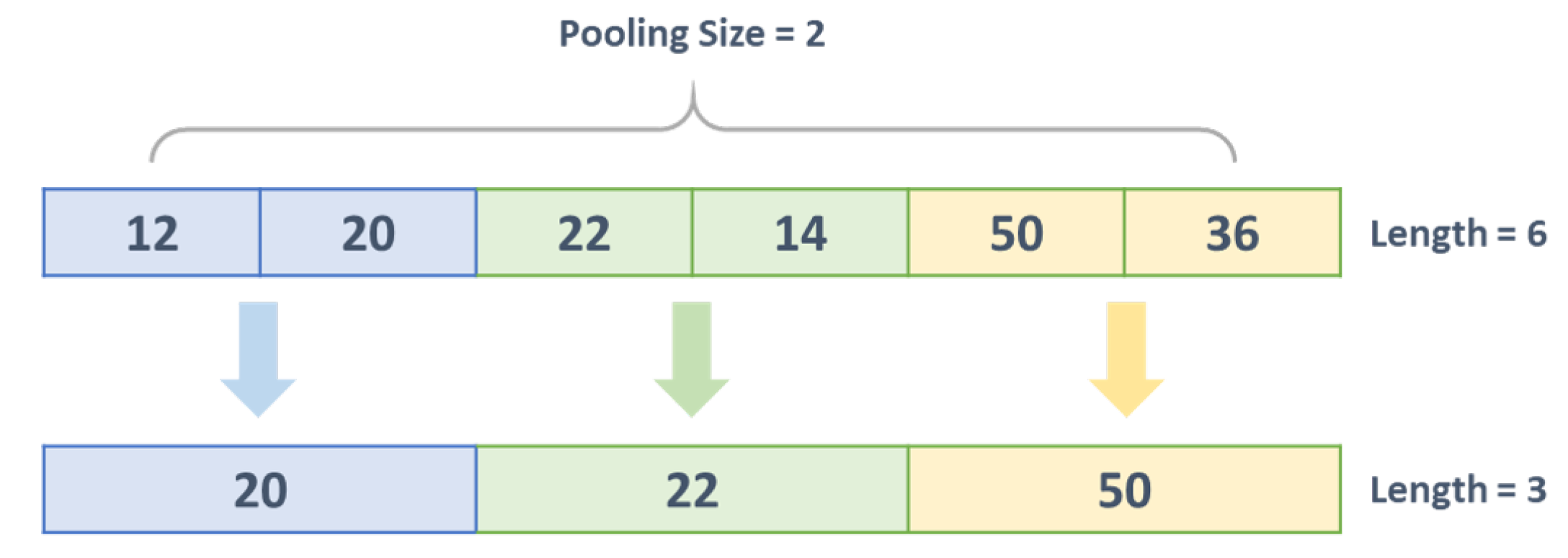
Two techniques, normalization and standardization, aim to transform the data by putting all the data points on the same scale in preparation for training [48]. Batch Normalization (BN) is a technique used to improve neural network efficiency and stability and prevent gradient vanishing and over-fitting [49]. BN is further used in feature maps to fix problems with internal covariance shift [50]. The change in the internal covariance is a change in the distribution of hidden unit values that slows convergence and requires careful initialization of network parameters [51]. BN normalizes the previous activation output by subtracting the batch-mean then dividing by the batch standard deviation. Therefore, each network-layer will learn a little more independently from other layers. BN enables us to use much higher learning rates and to take less care of initialization. It also works as a regularizer and eliminates the need for dropout in some cases and increases a neural network’s stability [52].

$$\mathrm{BN}\left(x_k\right)=\alpha \left(\frac{x_k-{\mu }_{\mathrm{B}}}{\sqrt{{\sigma }_{B^2}+\epsilon }}\right)+\beta$$

(2)

where, $\epsilon$ is a random noise for (stability), ${\mu }_{\mathrm{B}}$ represents the mini-batch mean, $\alpha$ is the mini-batch variance, $\sigma$ represents a scale parameter, and $\beta$ is the shifting parameter (offset) for the layer. Both $\alpha$ and $\beta$ are trainable and updated in an epoch-wise manner.

3.3. Pooling Layer

Pooling layers are crucial for the CNNs [44]. Methods for pooling can be considered down-samples to minimize the number of parameters while maintaining the major features to speed up the next stage since there are more feature maps in the downstream sampling phase, leading to an increased data dimensionality, which does not make calculations possible [43]. Therefore each feature map is processed at this phase with either (average or max) method [53]. The max-pooling method selects the highest parameters in the default window. At the same time, average-pooling is based on the pre-determined pooling window size as the output value.

Pooling methods are also intended to solve the issue of over-fitting. Although several pooling methods in CNNs can be used, the most common approach is max pooling [54]. Figure 3 shows the 1D max-pooling operation. The map is $\left(6\right)$ and the pooling is $\left(2\right)$ in size before pooling. The output values will be reduced to $\left(3\right)$, and the max values for the next network layer will be selected.

3.4. Dropout Layer

Using the dropout method can often resolve the problem of over-fitting during the training phase [55,56]. Network input information is transmitted from the input layer and the output layer passing through various hidden layers [23]. During training, weights are tuned and adjusted, where the dropout approach involves random neurons to be selected. Neurons are to be disabled during training so that randomly disabled neurons have no output values or values set to zero [57,58,59]. Connections are also temporarily removed from disabled neurons. The neural network can still function well, although some neurons are temporarily disabled. Over-fitting can be solved effectively with the random “dead neuron” selection process [41,56].

3.5. Fully Connected Layer

The fully-connected (FC) layer is a very special and vital component of convolutional neural networks, which have been very successful when it comes to computer vision [60]. The CNN process starts with convolution and pooling, breaks down the input into a vector of features, then independently analyses them [61]. This procedure leads to the final decision being fully-connected. The network’s earlier layers output is reshaped (flattened) into a single vector. Each of them represents the chance that a particular feature is a class label. Inputs are taken from the feature map, and weights are applied to determine the correct label. The output layer of FC [62] gives the final probabilities for every label.

3.6. Network Optimization

Neural network hyper-parameters shape how the network functions and determine its accuracy and validity. Hyper-parameters are an unsolved problem [63]. Optimizers are algorithms used to adjust the neural network properties, such as weight and learning rate, to minimize losses. The most popular method used to optimize deep learning networks is gradient descent [23]. Stochastic Gradient Descent (SGD) remains one of the most effective deep neural network optimization algorithms over the past century [64]. It performs computations across the entire dataset, which have been reported to be redundant and inefficient [23]. Various strategies and methods for improving the training process have been proposed to improve SGD performance, such as momentum and Nesterov acceleration [65]. Adaptive optimizations have become popular recently as they adjust the learning rates of parameters in different scales instead of directly regulating the overall phase sizes, resulting in a smoother training process and faster convergence. The adaptive learning rate is determined by dividing the gradients by a denominator, representing the square root of the global mean for previous gradient squares [66]. Many studies reported that AdaGrad gradients usually converge faster than vanilla SGD when the gradients are sparse [67]. However, its generalization performance is relativity poor [68]. Other adaptive algorithms, such as AdaDelta [69], RMSProp [70], and Adam [71] were mainly proposed to replace the denominator by the square root of the exponential moving average of past gradient squares. Adam has recently appeared in most academic papers since it converges way faster than other adaptive methods. Adam combines the advantages of SGD extensions, RMSProp, and AdaGrad. Adam and RMSprop have shown better optimization performance than SGD; they often lead to worse generalization performance [68,72,73,74].

Unlike Adam, which ignores the past gradients, we propose Exponential Adaptive Gradients (EAG) optimization, which is a combination of Adam, and AdaBound [74] exponentially accumulates the gradient information in the past during training to adaptively tune the learning rate and overcome Adam poor generalization and allow for convergence in both the convex and non-convex settings. Although Adam shows fast convergence in many tasks, it could lead the algorithm to local minima [75]. EAG does the exact opposite of Adam by measuring the past gradients exponentially more and progressively reducing the adaptability to present gradients, as shown in Algorithm 2. Extensive experiments have been made in the study to evaluate EAG performance compared to Adam and other adaptive methods in the domain of air pollution forecasting. We thoroughly prove the convergence of it in both the convex and non-convex settings. The most significant differences between Exponential Adaptive Gradients and Adam is that the previous gradients are multiplied by a constant greater than 1 and employ dynamic bounds on learning rates, which means that past information is accumulated rather than forgotten. The idea behind the Exponential Adaptive Gradients algorithm is to gradually decrease the adaptivity of the second moment to the latest gradients because when the parameters are close to the optimal points, they become sparse and noisy. Therefore, to maintain an accurate second moment, we would divide $v_t$ by ${\left(1+{\beta }^2\right)}^t-1$ in line (7).

$$\mathrm{Adam}:m_t={\beta }_1·m_{t-1}+\left(1-{\beta }_1\right)·g_t$$

(3)

$$\mathrm{AdaBound}:m_t={\beta }_{1t}·m_{t-1}+\left(1-{\beta }_{1t}\right)·g_t$$

(4)

Adam first momentum has the same form except for the constant $1-{\beta }_1$. Therefore the first order bias correction term is counter intuitive. Moreover, we have employed dynamic bounds on learning rates based on [74] to achieve a gradual and smooth transition from adaptive methods to SGD and give a theoretical proof of convergence in both convex and non-convex settings.

Algorithm 2. Proposed Exponential Adaptive Gradients (EAG) Algorithm.

1Input:$x\in F,{\left\{{\alpha }_t\right\}}_{t=1}^T,\left({\beta }_1,{\beta }_2\right)=\left(0.9,{10}^{-4}\right)$

2Initialize:$m_0=0,v_0=0$

3For$\mathit{t}=1$ to $\mathit{T}$ Do:

4        $g_t=▽f_t\left(x_t\right)$

5:        $m_t={\beta }_1·m_{t-1}+\left(1-{\beta }_1\right)·g_t$

6        $v_t=\left(1+{\beta }_2\right)v_{t-1}+{\beta }_2·g_t^2$

7        ${\widehat{v}}_t=v_t/\left[{\left(1+{\beta }_2\right)}^t-1\right]$ and $V_t=diag\left({\widehat{v}}_t\right)$

8        $x_{t+1}=\prod {}_{F,\sqrt[]{V_t}}\left(x_t-{\alpha }_t{m}_t/\sqrt[]{V_t}\right)$

9End For

4. Experiments

This section provides a description experiments environment, data pre-processing and the hyper-parameter configurations. All experiments were done on a Linux PC with i5-6300HQ CPU and 8 GB RAM. The use of PC GPU was unnecessary since computational cost of the 1D-CNN architecture is relatively low. The objective is to offer a model that is not so computationally expensive without affecting the level of accuracy. Scikit-learn [76] was used for data pre-processing alongside TensorFlow [76,77] to develop the baseline of all learning models.

4.1. Data Description and Pre-Processing

Air Pollution Index (API) is an effective measure that defines environmental air quality and provides easily understandable information on air pollution. Particulate matter $\left(P{M}_{10}\right)$, Carbon monoxide $\left(CO\right)$, ozone $\left(O_3\right)$, sulfur dioxide $\left(S{O}_2\right)$, and nitrogen dioxide $\left(N{O}_2\right)$ are the main sub-indices included in the information provided [78]. In terms of quality of air pollution, API had been adopted in Malaysia [79]. The API is a simple number ranged between 0 and ∞ reflecting the air quality levels associated with the effects on our health [80]. The study considers maximum daily API values received and obtained from the air monitoring station in Klang, Malaysia. Town of Klang is located approximately 32 km west of the capital Kuala Lumpur and covers about 573 ${\mathrm{km}}^2$ of land area. The Department of the Environment, Malaysia, provided the API records at the selected monitoring station. Air quality is not considered good if the API value is greater than 100 [78]. In contrast, at API values below 100 the air quality is good [81]. Classification of pollution level is based on (50, 100, 200, 300 and $300+$) breakpoints for APIs corresponding to (good, moderate, unhealthy, very unhealthy and hazardous), respectively.

$$\left[\begin{array}{cccc}{\delta }_1^1& {\delta }_1^2& \cdots & {\delta }_1^n\\ {\delta }_1^2& {\delta }_2^2& \cdots & {\delta }_2^n\\ {\delta }_1^3& {\delta }_3^3& \cdots & {\delta }_3^n\\ ⋮& ⋮& ⋮& ⋮\\ {\delta }_m^1& {\delta }_m^2& \cdots & {\delta }_m^n\end{array}\right]\to \left[\begin{array}{c}{r}_1^1\\ r_1^2\\ r_1^3\\ ⋮\\ r_m^1\end{array}\right]$$

(5)

where ${\delta }_i^j$ denotes instance of one-dimensional signals feature, $r_i$ is a corresponding output, $1\le i\le m,1\le j\le n$, m is represents the size of the dataset, n is the number of input features.

Figure 4 illustrates the distribution of API concentration, where the API concentration indicates the horizontal axis, and the vertical axis is the frequency. Meanwhile, the maximum, minimum, median, average, and standard deviation of API concentration are 7.0, 233.0, 54.0, 56.90, and 25.13, respectively. We used pre-processing techniques to normalize, split, and transform the data into a required shape to fit the proposed model.

Pre-processed data contribute to the improvement of the accuracy of the proposed model. The k-fold cross-validation (k-cv) [82] is one of the most popular techniques. Usually, in k-cv, the dataset is split into k folds. The prediction model is trained using $k-1$ folds, and the testing model will use the remaining fold. In k-cv, an $S_n$ dataset is randomly partitioned in similar size k-folds $N=\{f_1,\cdots ,f_n\}$. Finally, the k-cv error estimate is the average error value for each fold. Therefore, the k-CV error estimator depends on two factors: the training set and the folded partitions. Networks are equipped by adjusting the weight and bias of the connections on each layer. Continuing the training process until actual and the predicted output value are attained to a minimum error. The performance of the network is measured during training, validation, and testing.

4.2. Hyper-Parameter Selection

Tuning or optimizing hyper-parameters involves determining the values of each hyper-parameter that will help the model achieve the highest accuracy [83]. Normally, hyper-parameters used to be tuned manually by trial and error, which is a time-consuming task since it takes too much time to try the possible hyper-parameters that might give a good result. This is still very popular among researchers, and experienced operators may "guess" parameter values that might return a very high accuracy for deep learning models [23]. Tuning approaches commonly used include experimental methods, such as genetic algorithm (GA) [84], and particle swarm optimization (PSO) [85,86]. These methods take time because experimental methods include the approximation of value through numerous experiments [87]. GA and PSO are heuristic algorithms, and they are limited to dealing with a large-scale network. In this paper, we used grid search [88] which consisted of dividing hyper-parameter values into several steps to create a range grid and then cross all grid points to find the best grid hyper-parameter values.

It requires systematically checking several hyper-parameters values by retraining the model automatically for each parameter value [87]. It is useful because it maps the problem space and gives many solution choices. There are several hyper-parameters to train the proposed model, such as an optimizer, learning-rate, and filter size. We can manually search for these parameters. We also can employ advanced search methods, such as GridSearchCV. A class built on top of the scikit-learn framework, mainly for model parameters adjustment, is implemented by estimators. This approach searches for the best model and the best k-cv performance parameters for every training set. The grid-search cross-validation produces estimates of performance statistics for each point in the grid. Besides, different data split between the folds can create various optimal tuning parameters. Thus, the tuning parameter was selected with a mean $k-$ CV error, and we call it the optimal cross-validation option. Selected hyper-parameters are shown in

Table 1. Proposed model detailed parameters.

Layer	Type	Kernel × Filter	Other Parameters
1	Convolution1D	2 × 64	Activation = ReLU, Strides = 2
2	MaxPooling1D	—	Size = 2, Strides = 2
3	Convolution1D	2 × 128	Activation = ReLU, Strides = 2
4	MaxPooling1D	Size = 2, Strides = 2
5	Flatten	—	—
6	Dense	1 × 128	Activation = ReLU
8	Dropout	—	Rate = 0.3
9	Dense (Output)	{1 × 12}	Activation = Hyperbolic Tangent

.

All experiments reported in this section used a 5-fold cross-validation procedure to produce a fair comparison with the results. Different architectures have been developed to verify which is the most convenient to solve the API problem. However, Adam combines the advantages of two SGD extensions, RMSprop and Adagrad. In many tasks, adaptive optimization techniques generalize poorly compared to SGD, which led us to evaluate the optimizers’ performances on the proposed model. This led us to overcome this problem by combining Adam and AdaBound to overcome the poor generalization problem of adaptive methods. Because of its competitive performance and its ability to work well with limited tuning, Adam is used in many applications [72]. Adam has shown fast convergence in many runs; however, Adam’s fast convergence would lead the algorithm to local minimums. Exponential Adaptive Gradients (EAG) exponentially accumulate the gradient information during training with dynamic bounds on the learning rate to adaptively tune the learning rate and converge in both the convex and non-convex settings. Network weights with the lowest validation error were saved during training. Data preprocessing and hyper-parameters selection are discussed briefly in Section 4. Kernel’s initializer employs dynamic bounds on learning rates where the lower and upper bound are initialized as zero and infinity, respectively [74]. Several hyper-parameters were used to achieve the best forecast performance. A non-linear hyperbolic tangent (6) function is used for the final prediction of the output layer. Experiments were carried out to calculate and record the relevant indicators (MAE, RMSE, MAPE, and $R^2$), as shown in

Table 2. Effect of the number of filters on CNN model.

Filters	MAE	RMSE	MAPE	${\mathit{R}}^2$	Time(s)
32	2.407	2.7015	4.992	0.958	188.83
64	2.069	2.384	4.293	0.966	254.45
128	2.026	2.335	4.184	0.968	363.50
256	2.134	2.431	4.450	0.963	508.97
512	2.186	2.496	4.355	0.963	1013.34

.

$$\alpha \left(z\right)=\frac{1}{1+e^{-z}}$$

(6)

4.3. Evaluation Metrics

Prediction of API was targeted in this study. In order to assess the accuracy of the developed model, several statistical measures have been used. In this task, Root Mean Square Error ($RMSE$), Mean Absolute Error ($MAE$), and Pearson correlation ($R^2$) have been used as evaluation metrics. Each statistical measurement is shown in (7), (8) and (10) as mathematical representation, respectively, where $y_i$ is the actual value, $y_i^{{}^{\prime }}$ represents the predicted value, p is the number of dataset elements, $1<i\le p$. Values of $MAE$ and $RMSE$ are ranged between (zero and infinity). The closer the forecast to zero, the better the prediction. Pearson correlation values range from negative to positive 1. The nearer to 1, the better the forecasts [89,90].

$$MAE=\frac{1}{p}\sum _{i=1}^p\left|{\widehat{y}}_i-y_i\right|$$

(7)

$$RMSE=\sqrt{\frac{{\sum }_{i=1}^p{\left({\widehat{y}}_i-y_i\right)}^2}{p}}$$

(8)

$$MAPE=\frac{1}{N}\sum _{i=1}^N\left|\frac{y_i-{\widehat{y}}_i}{y_i}\right|·100$$

(9)

$$R^2=\frac{p\left({\sum }_{i=1}^p{\widehat{y}}_i{y}_i\right)-\left({\sum }_{i=1}^p{\widehat{y}}_i\right)\left({\sum }_{i=1}^p{y}_i\right)}{\sqrt{\left(p{\sum }_{i=1}^p{y}_i^2-{\left(p{\sum }_{i=1}^p{y}_i\right)}^2\right)\left(p{\sum }_{i=1}^p{\widehat{y}}_i^2-{\left(p{\sum }_{i=1}^p{\widehat{y}}_i\right)}^2\right)}}$$

(10)

5. Results and Discussion

One Dimensional CNNs are particularly promising in time series predictions since they can map the input to output sequences with past contexts in their internal state. They can be described as several copies of the same neural network. They transmit information to their successor and form a chain-like architecture, which is naturally connected to the sequences [91]. Moreover, 1D-CNN combines both feature extraction and prediction into one learning body-block, which solves the problem of handcrafted feature selection in other networks, thus maximizing prediction performance. The proposed architecture and hyper-parameter selection, based on cross-validation and grid search, can be shown below in Table 1.

Experiments have shown that the number of filters has a significant impact on feature extraction. Table 2 shows the multi-convolution of the same input against various numbers of filter sizes. We can see that, as the number of filters increases, the accuracy also improves. However, the improvement comes at the cost of computational time. Table 2 shows the model performance under a different number of convolution filters. The performance of the proposed model was empirically improved by determining the optimal filter size in the range of 64 and 128. Moreover, overall performance was best using 64 filters for all developed models since it gives satisfactory results with less computational time.

As can be observed in Figure 5, despite the initial fast convergence of Adam, their final loss could not catch up with EAG. However, other optimizers converged faster than EAG but yielded similar performances. As observed, although Adam was fast at the beginning, its test accuracy stagnated after the second learning rate decrease. RMSprop performed even worse than Adam. On the other hand, EAG converged without increasing the loss in most of the runs. However, more time consumed, as shown in Figure 5 and Figure 6.

The selected network loss function (MAE) has shown that the training dataset loss function is not much lower than the validation dataset loss function, meaning that network did not overfit during the training process. Since we are focusing on one dimensional CNN and it is performing against counterparts approaches, such as LSTM, a network of other architecture was designed for efficiency comparison of the proposed system in the related domain [6]. The outcomes of the comparison results can be shown in

Table 3. Effect of the number of iterations on models and convergence time.

Iterations	LSTM				CNN
	MAE	RMSE	MAPE	${\mathit{R}}^{\mathbf{2}}$	MAE	RMSE	MAPE	${\mathit{R}}^{\mathbf{2}}$
1	20.699	22.357	35.649	−0.768	9.732	11.491	17.422	0.541
2	8.061	8.616	13.855	0.710	5.336	5.985	10.413	0.847
4	6.440	7.026	11.421	0.819	4.809	5.128	9.622	0.872
8	5.090	5.482	9.340	0.883	3.768	4.106	7.390	0.916
16	4.253	4.443	7.457	0.921	3.100	3.420	6.053	0.941
32	3.005	3.358	5.702	0.950	2.841	3.113	5.550	0.949
64	2.999	3.228	5.624	0.956	2.423	2.714	5.021	0.959
128	2.997	3.277	5.117	0.944	2.291	2.600	4.632	0.962
256	2.951	3.170	5.222	0.955	2.023	2.341	4.212	0.969
512	2.103	2.392	4.266	0.969	2.044	2.367	4.178	0.968
1024	2.636	2.865	4.716	0.963	1.894	2.222	3.765	0.974

.

Different optimizers have been selected to optimize the developed model. The performance and outcomes are displayed in Figure 5 and Figure 6. Adaptive optimization algorithms, such as Adam and RMSprop, in many cases, have shown better performance. Recent studies, however, indicate that generalization performance is often worse than SGD, especially for deep neural networks. Adam and RMSprop have shown a great result in a few runs and unsatisfactory performance in other runs. However, the lack of generalization performance of adaptive methods, such as Adam and RMSPROP, might be caused by unstable or extreme learning rates and suggested that the modest learning rates of adaptive methods can lead to undesirable non-convergence [74]. Adam algorithm was found to be the best optimizer in terms of speed but not error rate. In addition, the hyperbolic tangent activation function generated better models than the sigmoid activation function in the output layer.

Table 4. Comparison of different optimization algorithms.

Optimizer	Evaluation	LSTM	CNN
Adadelta	MAE (Loss)	3.270	3.118
	RMSE	3.480	3.342
	MAPE	5.915	5.785
	$R^2$	0.947	0.946
Adagrad	MAE (Loss)	3.215	2.934
	RMSE	3.430	3.181
	MAPE	5.966	6.012
	$R^2$	0.952	0.943
Adamax	MAE (Loss)	2.918	2.502
	RMSE	3.150	2.784
	MAPE	5.016	5.180
	$R^2$	0.950	0.957
Nadam	MAE (Loss)	3.142	2.728
	RMSE	3.360	2.976
	MAPE	5.428	5.616
	$R^2$	0.947	0.950
RMSprop	MAE (Loss)	2.609	2.893
	RMSE	2.861	3.124
	MAPE	4.650	5.419
	$R^2$	0.956	0.951
Adam	MAE (Loss)	2.541	2.414
	RMSE	2.803	2.677
	MAPE	4.641	4.760
	$R^2$	0.954	0.959
EAG	MAE (Loss)	2.374	2.034
	RMSE	2.631	2.344
	MAPE	4.347	4.214
	$R^2$	0.954	0.967

shows the MAE, RMSE, MAPE, and $R^2$ overall results obtained by both approaches—LSTM and developed 1D-CNN. The generated 1D-CNN model revealed an average of MAE of 2.036, RMSE of 2.354, and $R^2$ of 0.966 over the test dataset for 25 independent iterations. The fitness of the developed model 1D-CNN was optimized by EAG and gave excellent and stable results in all iterations with the lowest average error rate compared to other optimizers. The prediction results are displayed in Table 4. EAG was selected with a learning rate of $\alpha =0.0114$ based on grid search as a primary optimizer for the developed models.

The boxplot of the prediction deviation is shown in Figure 7. The height of the box partly reflects the fluctuation in the deviation data, and the flatter the box, the more centralized the data are. Figure 8 represents the absolute difference between actual and forecasted values for each prediction model. The number of outliers in the other optimizers and the LSTM model was higher than the number of outliers in the 1D-CNN model. This can be referred to as the high RMSE obtained. In terms of the comparison analysis, the proposed method outperforms other models, including mainstream approaches, such as LSTM, not only in terms of performance but also time complexity and consistency. It fully proves the effectiveness and superiority of the 1D convects in non-convex optimization. We have demonstrated that the non-convex optimization performed better in all 25 independent runs, unlike other optimizers that have shown a big difference in MAE and RMSE in every run, since adaptive methods tend to converge quickly towards sharper minima. In comparison, flatter minima generalize better than sharper ones. However, we observed that the solutions found by adaptive methods generalize worse (often significantly worse) even when these solutions have better training performance. Therefore, as a part of future work, ensemble techniques could be investigated to combine each optimizer’s efficiencies with building up a super model.

Similarly, Table 4 shows the four measurement indices for each model. The RMSE value of the proposed 1D-CNN–EAG model is lower than the models. The MAE and RMSE values of both Adam and RMSprop models are slightly lower than that of LSTM models, which can be clearly shown in Figure 9a,b. It represents the values of RMSE of each optimizer and show that EAG has the lower average by far than that of other optimizers. In terms of training time and complexity, 1D-CNN is three times faster on average for every epoch. LSTM could not keep up the same performance in training time comparison. The average 1D-CNN time was approximately 4–7 s for every epoch, while LSTM took roughly 18–27 s for one epoch.

To compare the prediction effect of each model more intuitively, the scatter plots of observed and predicted API concentrations during the whole test set are illustrated in Figure 10. The distribution between predicted and observed values can be seen in Figure 10a,b. Apparently, variants of 1D-CNN (Figure 10b) show better results than LSTM (a). Compared with all the models described above, the proposed model is more sensitive to sharp changes. Which mainly attributed to the existence of convolution networks that capture richer local change information. API was correctly forecast on most peaks, especially in days with very high averages with a good RMSE value. We investigated the influence of epoch size on various models. By increasing iterations, the model loss gradually decreases, and MAE reaches its lowest at the value of 1.894 at all experiments runs, as shown in Table 3.

Checkpointing has been utilized to save the network weights only when there is an improvement in the validation dataset. The weights are stored in a file if and only if the validation accuracy improves. It will ensure that the best model is saved. Moreover, all models used the early-stopping condition that stops and interrupts the training if the validation loss on the validation information does not change in 12 epochs of training. We also observed that model error remains unchanged as the lookup size increases. Finally, results have shown that 1D-CNN and EAG optimizer can learn complex patterns better than other predictive models. From the above results, we have demonstrated that a 1D-CNN–EAG can successfully predict the API. Prediction for API time series under different experimental conditions has been carried out. Although the EAG optimizer obtained the best results, performance in terms of time complexity was observed. Certain functions with minor changes to our proposed 1D-CNN–EAG architecture may also be appealing to many other domains.

It has been demonstrated in many applications that 1D-CNNs are relatively easier to train and deliver minimal computational complexity while achieving cutting-edge performance, especially now with convergence in both the convex and non-convex settings. This paper demonstrated the benefits of utilizing machine learning techniques for predictive analytics that will create enormous opportunities for having deeply beneficial influences on society (healthcare, education, sustainability, etc.). Additionally, this method could be applied to other contexts in different countries. We are optimistic that researchers and public agencies can continue to expand and test this method to improve environmental sustainability.

The obtained network training dataset is the key downside of the neural network. Suppose training data are insufficient and not appropriate. In that case, the network will quickly learn the dataset bias and generally make poor predictions of data with trends the training data have never seen. Besides, it is typically more difficult to track back if a network does not function as intended. We have used only the data provided in this paper for network training, which may lead to bias by overlooking the effects of unusual situations. Perhaps a more effective approach would be used to train the network in a semi-supervised fashion to boost network performance on unseen data by using limited actual data and data generated during the training. It will also increase data from different sectors, such as transportation and industry, on air pollutants to improve the learning model. This will be used in our future research topics [92].

Future work will focus more on effective methods to adjust hyper-parameters and the use of feature selection [92,93]. It will help to remove redundant features and thus obtain better performance. Additionally, future work will investigate more accurate methods of hyper-parameter tuning techniques. Although the grid search can be utilized, the search range needs to be manually updated since values are always fixed. It will be important to find an adaptive way to automatically adjust the hyper-parameters searching process and make the neural network architecture evolve by automatically reshaping, adding, and removing various layers. Additionally, this work will consider hybrid networks [94] to merge the advantages of different approaches.

6. Conclusions

Deep One-Dimensional Deep Convolutional Neural Network and Exponential Adaptive Gradient optimization (1D-CNN–EAG) have been proposed to predict the Air Pollution Index (API) for Klang city, Malaysia. Thus, using grid search cross-validation to find optimal hyper-parameters for the proposed model. The performances of the proposed model have been investigated. The prediction process involves following steps. First, the dataset was normalized and then divided into $5-$ folds using cross-validation, a classifier is learned using $k-1$ folds, and an error value is calculated by testing the model on the remaining fold. Thus, using grid search cross-validation to find optimal hyper-parameters for the proposed model. The performance of the models was evaluated by four indicators—MAE of 2.036, RMSE of 2.354, and $R^2$ of 0.966 with a 1.14% improvement in overall performance. Besides, these results are compared with other state-of-the-art approaches. The ability of 1D-CNN–EAG to perform in API prediction was highlighted in this study and proved the capability of convolutional neural networks to perform a daily API prediction. The study has shown that the 1D-CNN outperformed all alternative approaches. Future research involves combining the diversities of the models with ensemble techniques alongside additional data from different locations and repositories, and looking at a more accurate method of hyper-parameters selection.

References

1. Huang, C.J.; Kuo, P.H. A deep cnn-lstm model for particulate matter (PM2.5) forecasting in smart cities. Sensors 2018, 18, 2220. [Google Scholar] [CrossRef] [PubMed] [Green Version]
2. Bourdrel, T.; Bind, M.A.; Béjot, Y.; Morel, O.; Argacha, J.F. Cardiovascular effects of air pollution. Arch. Cardiovasc. Dis. 2017, 110, 634–642. [Google Scholar] [CrossRef] [PubMed]
3. Rahman, N.H.A.; Lee, M.H.; Suhartono, M. Evaluation performance of time series approach for forecasting air pollution index in johor, malaysia. Sains Malays. 2016, 45, 1625–1633. [Google Scholar]
4. Özkaynak, H.; Glenn, B.; Qualters, J.R.; Strosnider, H.; Mcgeehin, M.A.; Zenick, H. Summary and findings of the EPA and CDC symposium on air pollution exposure and health. J. Expo. Sci. Environ. Epidemiol. 2009, 19, 19–29. [Google Scholar] [CrossRef] [PubMed] [Green Version]
5. Spiru, P.; Simona, P.L. A review on interactions between energy performance of the buildings, outdoor air pollution and the indoor air quality. Energy Procedia 2017, 128, 179–186. [Google Scholar] [CrossRef]
6. Haidar, A.; Verma, B. Monthly rainfall forecasting using one-dimensional deep convolutional neural network. IEEE Access 2018, 6, 69053–69063. [Google Scholar] [CrossRef]
7. Alyousifi, Y.; Othman, M.; Faye, I.; Sokkalingam, R.; Silva, P.C. Markov Weighted Fuzzy Time-Series Model Based on an Optimum Partition Method for Forecasting Air Pollution. Int. J. Fuzzy Syst. 2020, 22, 1468–1486. [Google Scholar] [CrossRef]
8. Szczurek, A.; Maciejewska, M.; Połoczański, R.; Teuerle, M.; Wyłomańska, A. Dynamics of carbon dioxide concentration in indoor air. Stoch. Environ. Res. Risk Assess. 2015, 29, 2193–2199. [Google Scholar] [CrossRef] [Green Version]
9. Choon, S.W.; Ong, H.B.; Tan, S.H. Does risk perception limit the climate change mitigation behaviors? Environ. Dev. Sustain. 2019, 21, 1891–1917. [Google Scholar] [CrossRef]
10. Razak, M.I.M.; Ahmad, I.; Bujang, I.; Talib, A.H.; Ibrahim, Z. Economics of air pollution in Malaysia. Int. J. Humanit. Soc. Sci. 2013, 3, 173–177. [Google Scholar]
11. Alyousifi, Y.; Othman, M.; Sokkalingam, R.; Faye, I.; Silva, P.C. Predicting Daily Air Pollution Index Based on Fuzzy Time Series Markov Chain Model. Symmetry 2020, 12, 293. [Google Scholar] [CrossRef] [Green Version]
12. Wong, T.W.; San Tam, W.W.; Yu, I.T.S.; Lau, A.K.H.; Pang, S.W.; Wong, A.H. Developing a risk-based air quality health index. Atmos. Environ. 2013, 76, 52–58. [Google Scholar] [CrossRef]
13. Jiang, D.; Zhang, Y.; Hu, X.; Zeng, Y.; Tan, J.; Shao, D. Progress in developing an ANN model for air pollution index forecast. Atmos. Environ. 2004, 38, 7055–7064. [Google Scholar] [CrossRef]
14. Aghamohammadi, N.; Isahak, M. Climate Change and Air Pollution in Malaysia. In Climate Change and Air Pollution; Springer: New York, NY, USA, 2018; pp. 241–254. [Google Scholar]
15. Donnelly, A.; Misstear, B.; Broderick, B. Real time air quality forecasting using integrated parametric and non-parametric regression techniques. Atmos. Environ. 2015, 103, 53–65. [Google Scholar] [CrossRef]
16. Zhou, Q.; Jiang, H.; Wang, J.; Zhou, J. A hybrid model for PM2.5 forecasting based on ensemble empirical mode decomposition and a general regression neural network. Sci. Total Environ. 2014, 496, 264–274. [Google Scholar] [CrossRef]
17. Abdulkadir, S.J.; Yong, S.P. Unscented kalman filter for noisy multivariate financial time-series data. In International Workshop on Multi-Disciplinary Trends in Artificial Intelligence; Springer: York, NY, USA, 2013; pp. 87–96. [Google Scholar]
18. Abdulkadir, S.J.; Yong, S.P. Scaled UKF–NARX hybrid model for multi-step-ahead forecasting of chaotic time series data. Soft Comput. 2015, 19, 3479–3496. [Google Scholar] [CrossRef]
19. Abdulkadir, S.J.; Yong, S.P.; Marimuthu, M.; Lai, F.W. Hybridization of ensemble Kalman filter and non-linear auto-regressive neural network for financial forecasting. In Mining Intelligence and Knowledge Exploration; Springer: York, NY, USA, 2014; pp. 72–81. [Google Scholar]
20. Kamaruzzaman, A.; Saudi, A.; Azid, A.; Balakrishnan, A.; Abu, I.; Amin, N.; Rizman, Z. Assessment on air quality pattern: A case study in Putrajaya, Malaysia. J. Fundam. Appl. Sci. 2017, 9, 789–800. [Google Scholar] [CrossRef] [Green Version]
21. Tsai, Y.T.; Zeng, Y.R.; Chang, Y.S. Air pollution forecasting using RNN with LSTM. In Proceedings of the 2018 IEEE 16th Intl Conf on Dependable, Autonomic and Secure Computing, 16th Intl Conf on Pervasive Intelligence and Computing, 4th Intl Conf on Big Data Intelligence and Computing and Cyber Science and Technology Congress (DASC/PiCom/DataCom/CyberSciTech), IEEE, Athens, Greece, 12–15 August 2018; pp. 1074–1079. [Google Scholar]
22. Salman, A.G.; Heryadi, Y.; Abdurahman, E.; Suparta, W. Single layer & multi-layer long short-term memory (LSTM) model with intermediate variables for weather forecasting. Procedia Comput. Sci. 2018, 135, 89–98. [Google Scholar]
23. LeCun, Y.; Bengio, Y.; Hinton, G. Deep learning. Nature 2015, 521, 436–444. [Google Scholar] [CrossRef]
24. Abimannan, S.; Chang, Y.S.; Lin, C.Y. Air Pollution Forecasting Using LSTM-Multivariate Regression Model. In International Conference on Internet of Vehicles; Springer: New York, NY, USA, 2019; pp. 318–326. [Google Scholar]
25. Chang, Y.S.; Chiao, H.T.; Abimannan, S.; Huang, Y.P.; Tsai, Y.T.; Lin, K.M. An LSTM-based aggregated model for air pollution forecasting. Atmos. Pollut. Res. 2020, 11, 1451–1463. [Google Scholar] [CrossRef]
26. Abdulkadir, S.J.; Yong, S.P. Empirical analysis of parallel-NARX recurrent network for long-term chaotic financial forecasting. In Proceedings of the 2014 International Conference on Computer and Information Sciences (ICCOINS), IEEE, Kuala Lumpur, Malaysia, 3–5 June 2014; pp. 1–6. [Google Scholar]
27. Abdulkadir, S.J.; Yong, S.P.; Foong, O.M. Variants of Particle Swarm Optimization in Enhancing Artificial Neural Networks. Aust. J. Basic Appl. Sci. 2013, 7, 388–400. [Google Scholar]
28. Abdulkadir, S.J.; Yong, S.P.; Zakaria, N. Hybrid neural network model for metocean data analysis. J. Inform. Math. Sci. 2016, 8, 245–251. [Google Scholar]
29. Abdulkadir, S.J.; Yong, S.P.; Alhussian, H. An enhanced ELMAN-NARX hybrid model for FTSE Bursa Malaysia KLCI index forecasting. In Proceedings of the 2016 3rd International Conference on Computer and Information Sciences (ICCOINS), Kuala Lumpur, Malaysia, 15–17 August 2016; pp. 304–309. [Google Scholar]
30. Abdulkadir, S.J.; Alhussian, H.; Nazmi, M.; Elsheikh, A.A. Long Short Term Memory Recurrent Network for Standard and Poor’s 500 Index Modelling. Int. J. Eng. Technol. 2018, 7, 25–29. [Google Scholar] [CrossRef]
31. Abdulkadir, S.J.; Yong, S.P. Lorenz time-series analysis using a scaled hybrid model. In Proceedings of the 2015 International Symposium on Mathematical Sciences and Computing Research (iSMSC), Ipon, Malaysia, 19–20 May 2015; pp. 373–378. [Google Scholar]
32. Pysal, D.; Abdulkadir, S.J.; Shukri, S.R.M.; Alhussian, H. Classification of children’s drawing strategies on touch-screen of seriation objects using a novel deep learning hybrid model. Alex. Eng. J. 2020. [Google Scholar] [CrossRef]
33. Wang, B.; Yan, Z.; Luo, H.; Li, T.; Lu, J.; Zhang, G. Deep uncertainty learning: A machine learning approach for weather forecasting. CoRR 2018, 19, 2087–2095. [Google Scholar]
34. Xie, J. Deep neural network for PM2.5 pollution forecasting based on manifold learning. In Proceedings of the 2017 International Conference on Sensing, Diagnostics, Prognostics, and Control (SDPC), Shanghai, China, 16–18 August 2017; pp. 236–240. [Google Scholar]
35. Athira, V.; Geetha, P.; Vinayakumar, R.; Soman, K. Deepairnet: Applying recurrent networks for air quality prediction. Procedia Comput. Sci. 2018, 132, 1394–1403. [Google Scholar]
36. Yan, L.; Wu, Y.; Yan, L.; Zhou, M. Encoder-decoder model for forecast of PM2.5 concentration per hour. In Proceedings of the 2018 1st International Cognitive Cities Conference (IC3), Okinawa, Japan, 7–9 August 2018; pp. 45–50. [Google Scholar]
37. Coşkun, M.; YILDIRIM, Ö.; Ayşegül, U.; Demir, Y. An overview of popular deep learning methods. Eur. J. Technol. 2017, 7, 165–176. [Google Scholar] [CrossRef] [Green Version]
38. Bengio, Y.; Goodfellow, I.; Courville, A. Deep Learning; MIT Press: Cambridge, MA, USA, 2017. [Google Scholar]
39. Huang, S.; Tang, J.; Dai, J.; Wang, Y. Signal status recognition based on 1DCNN and its feature extraction mechanism analysis. Sensors 2019, 19, 2018. [Google Scholar] [CrossRef] [Green Version]
40. Zhang, B.; Quan, C.; Ren, F. Study on CNN in the recognition of emotion in audio and images. In Proceedings of the 2016 IEEE/ACIS 15th International Conference on Computer and Information Science (ICIS), Okayama, Japan, 26–29 June 2016; pp. 1–5. [Google Scholar]
41. Schmidhuber, J. Deep learning in neural networks: An overview. Neural Netw. 2015, 61, 85–117. [Google Scholar] [CrossRef] [Green Version]
42. Zhang, W.; Peng, G.; Li, C.; Chen, Y.; Zhang, Z. A new deep learning model for fault diagnosis with good anti-noise and domain adaptation ability on raw vibration signals. Sensors 2017, 17, 425. [Google Scholar] [CrossRef] [PubMed]
43. Wang, H.; Liu, Z.; Peng, D.; Qin, Y. Understanding and Learning Discriminant Features based on Multi-Attention 1DCNN for Wheelset Bearing Fault Diagnosis. IEEE Trans. Ind. Inform. 2019, 16, 5735–5745. [Google Scholar] [CrossRef]
44. Huang, S.; Tang, J.; Dai, J.; Wang, Y.; Dong, J. 1DCNN Fault Diagnosis Based on Cubic Spline Interpolation Pooling. Shock Vib. 2020, 2020. [Google Scholar] [CrossRef] [Green Version]
45. Soon, F.C.; Khaw, H.Y.; Chuah, J.H.; Kanesan, J. Hyper-parameters optimisation of deep CNN architecture for vehicle logo recognition. IET Intell. Transp. Syst. 2018, 12, 939–946. [Google Scholar] [CrossRef] [Green Version]
46. Zhao, X.; Solé-Casals, J.; Li, B.; Huang, Z.; Wang, A.; Cao, J.; Tanaka, T.; Zhao, Q. Classification of Epileptic IEEG Signals by CNN and Data Augmentation. In Proceedings of the ICASSP 2020–2020 IEEE International Conference on Acoustics, Speech and Signal Processing (ICASSP), Barcelona, Spain, 4–8 May 2020; pp. 926–930. [Google Scholar]
47. Eren, L.; Ince, T.; Kiranyaz, S. A generic intelligent bearing fault diagnosis system using compact adaptive 1D CNN classifier. J. Signal Process. Syst. 2019, 91, 179–189. [Google Scholar] [CrossRef]
48. Zhao, J.; Mao, X.; Chen, L. Speech emotion recognition using deep 1D & 2D CNN LSTM networks. Biomed. Signal Process. Control 2019, 47, 312–323. [Google Scholar]
49. Shao, S.; Wang, P.; Yan, R. Generative adversarial networks for data augmentation in machine fault diagnosis. Comput. Ind. 2019, 106, 85–93. [Google Scholar] [CrossRef]
50. Abdoli, S.; Cardinal, P.; Koerich, A.L. End-to-end environmental sound classification using a 1D convolutional neural network. Expert Syst. Appl. 2019, 136, 252–263. [Google Scholar] [CrossRef] [Green Version]
51. Courville, A. Recurrent Batch Normalization. arXiv 2016, arXiv:1603.09025. [Google Scholar]
52. Meliboev, A.; Alikhanov, J.; Kim, W. 1D CNN Based Network Intrusion Detection with Normalization on Imbalanced Data. arXiv 2020, arXiv:2003.00476. [Google Scholar]
53. Wang, S.; Jiang, Y.; Hou, X.; Cheng, H.; Du, S. Cerebral micro-bleed detection based on the convolution neural network with rank based average pooling. IEEE Access 2017, 5, 16576–16583. [Google Scholar] [CrossRef]
54. Zhao, J.; Mao, X.; Chen, L. Learning deep features to recognise speech emotion using merged deep CNN. IET Signal Process. 2018, 12, 713–721. [Google Scholar] [CrossRef]
55. Lv, M.; Xu, W.; Chen, T. A hybrid deep convolutional and recurrent neural network for complex activity recognition using multimodal sensors. Neurocomputing 2019, 362, 33–40. [Google Scholar] [CrossRef]
56. Jeon, B.; Park, N.; Bang, S. Dropout Prediction over Weeks in MOOCs via Interpretable Multi-Layer Representation Learning. arXiv 2020, arXiv:2002.01598. [Google Scholar]
57. Fu, Q.; Niu, D.; Zang, Z.; Huang, J.; Diao, L. Multi-Stations’ Weather Prediction Based on Hybrid Model Using 1D CNN and Bi-LSTM. In Proceedings of the 2019 Chinese Control Conference (CCC), Guangzhou, China, 27–30 July 2019; pp. 3771–3775. [Google Scholar]
58. Gal, Y.; Ghahramani, Z. A theoretically grounded application of dropout in recurrent neural networks. In Advances in Neural Information Processing Systems; Barcelona, Spain, 2016; pp. 1019–1027. [Google Scholar]
59. Xiong, J.; Zhang, K.; Zhang, H. A Vibrating Mechanism to Prevent Neural Networks from Overfitting. In Proceedings of the 2019 15th International Wireless Communications & Mobile Computing Conference (IWCMC), Tangier, Morocco, 24–28 June 2019; pp. 1737–1742. [Google Scholar]
60. Swapna, G.; Kp, S.; Vinayakumar, R. Automated detection of diabetes using CNN and CNN-LSTM network and heart rate signals. Procedia Comput. Sci. 2018, 132, 1253–1262. [Google Scholar]
61. Fukuoka, R.; Suzuki, H.; Kitajima, T.; Kuwahara, A.; Yasuno, T. Wind Speed Prediction Model Using LSTM and 1D-CNN. J. Signal Process. 2018, 22, 207–210. [Google Scholar] [CrossRef] [Green Version]
62. Soni, S.; Dey, S.; Manikandan, M.S. Automatic Audio Event Recognition Schemes for Context-Aware Audio Computing Devices. In Proceedings of the 2019 Seventh International Conference on Digital Information Processing and Communications (ICDIPC), Trabzon, Turkey, 2–4 May 2019; pp. 23–28. [Google Scholar]
63. Tsirikoglou, P.; Abraham, S.; Contino, F.; Lacor, C.; Ghorbaniasl, G. A hyperparameters selection technique for support vector regression models. Appl. Soft Comput. 2017, 61, 139–148. [Google Scholar] [CrossRef]
64. Zhang, Z. Improved adam optimizer for deep neural networks. In Proceedings of the 2018 IEEE/ACM 26th International Symposium on Quality of Service (IWQoS), Banff, AB, Canada, 4–6 June 2018; pp. 1–2. [Google Scholar]
65. Botev, A.; Lever, G.; Barber, D. Nesterov’s accelerated gradient and momentum as approximations to regularised update descent. In Proceedings of the 2017 International Joint Conference on Neural Networks (IJCNN), Anchorage, Alaska, USA, 14–19 May 2017; pp. 1899–1903. [Google Scholar]
66. Ruder, S. An overview of gradient descent optimization algorithms. arXiv 2016, arXiv:1609.04747. [Google Scholar]
67. Duchi, J.; Hazan, E.; Singer, Y. Adaptive subgradient methods for online learning and stochastic optimization. J. Mach. Learn. Res. 2011, 12, 2121–2159. [Google Scholar]
68. Reddi, S.J.; Kale, S.; Kumar, S. On the convergence of adam and beyond. arXiv 2019, arXiv:1904.09237. [Google Scholar]
69. Zeiler, M.D. Adadelta: An adaptive learning rate method. arXiv 2012, arXiv:1212.5701. [Google Scholar]
70. Tieleman, T.; Hinton, G. Lecture 6.5-rmsprop: Divide the gradient by a running average of its recent magnitude. Coursera Neural Netw. Mach. Learn. 2012, 4, 26–31. [Google Scholar]
71. Kingma, D.P.; Ba, J. Adam: A method for stochastic optimization. arXiv 2014, arXiv:1412.6980. [Google Scholar]
72. Wilson, A.C.; Roelofs, R.; Stern, M.; Srebro, N.; Recht, B. The marginal value of adaptive gradient methods in machine learning. In Advances in Neural Information Processing Systems; The MIT Press: Long Beach, CA, USA, 2017; pp. 4148–4158. [Google Scholar]
73. Shazeer, N.; Stern, M. Adafactor: Adaptive learning rates with sublinear memory cost. arXiv 2018, arXiv:1804.04235. [Google Scholar]
74. Luo, L.; Xiong, Y.; Liu, Y.; Sun, X. Adaptive gradient methods with dynamic bound of learning rate. arXiv 2019, arXiv:1902.09843. [Google Scholar]
75. Wierichs, D.; Gogolin, C.; Kastoryano, M. Avoiding local minima in variational quantum eigensolvers with the natural gradient optimizer. arXiv 2020, arXiv:2004.14666. [Google Scholar]
76. Géron, A. Hands-On Machine Learning with Scikit-Learn, Keras, and TensorFlow: Concepts, Tools, and Techniques to Build Intelligent Systems; O’Reilly Media: Sebastopol, CA, USA, 2019. [Google Scholar]
77. Abadi, M.; Barham, P.; Chen, J.; Chen, Z.; Davis, A.; Dean, J.; Devin, M.; Ghemawat, S.; Irving, G.; Isard, M.; et al. Tensorflow: A system for large-scale machine learning. In Proceedings of the 12th USENIX Symposium on Operating Systems Design and Implementation ({OSDI} 16), Savannah, GA, USA, 2–4 November 2016; pp. 265–283. [Google Scholar]
78. Ahmad, Z.; Rahim, N.A.; Bahadori, A.; Zhang, J. Air polluiton index prediction using multiple neural networks. IIUM Eng. J. 2017, 18, 1–12. [Google Scholar] [CrossRef]
79. Rani, N.L.A.; Azid, A.; Khalit, S.I.; Juahir, H.; Samsudin, M.S. Air Pollution Index Trend Analysis in Malaysia, 2010–15. Pol. J. Environ. Stud. 2018, 27, 801–807. [Google Scholar] [CrossRef]
80. Sahani, M.; Zainon, N.A.; Mahiyuddin, W.R.W.; Latif, M.T.; Hod, R.; Khan, M.F.; Tahir, N.M.; Chan, C.C. A case-crossover analysis of forest fire haze events and mortality in Malaysia. Atmos. Environ. 2014, 96, 257–265. [Google Scholar] [CrossRef]
81. Zakaria, U.; Saudi, A.; Abu, I.; Azid, A.; Balakrishnan, A.; Amin, N.; Rizman, Z. The assessment of ambient air pollution pattern in Shah Alam, Selangor, Malaysia. J. Fundam. Appl. Sci. 2017, 9, 772–788. [Google Scholar] [CrossRef] [Green Version]
82. Krstajic, D.; Buturovic, L.J.; Leahy, D.E.; Thomas, S. Cross-validation pitfalls when selecting and assessing regression and classification models. J. Cheminform. 2014, 6, 1–15. [Google Scholar] [CrossRef] [Green Version]
83. Bergstra, J.; Bengio, Y. Random search for hyper-parameter optimization. J. Mach. Learn. Res. 2012, 13, 281–305. [Google Scholar]
84. Levy, E.; David, O.E.; Netanyahu, N.S. Genetic algorithms and deep learning for automatic painter classification. In Proceedings of the 2014 Annual Conference on Genetic and Evolutionary Computation, Vancouver, BC, Canada, July 2014; pp. 1143–1150. [Google Scholar]
85. Fornarelli, G.; Giaquinto, A. Adaptive particle swarm optimization for CNN associative memories design. Neurocomputing 2009, 72, 3851–3862. [Google Scholar] [CrossRef]
86. Syulistyo, A.R.; Purnomo, D.M.J.; Rachmadi, M.F.; Wibowo, A. Particle swarm optimization (PSO) for training optimization on convolutional neural network (CNN). J. Ilmu Komput. Dan Inf. 2016, 9, 52–58. [Google Scholar] [CrossRef]
87. Bhat, P.C.; Prosper, H.B.; Sekmen, S.; Stewart, C. Optimizing event selection with the random grid search. Comput. Phys. Commun. 2018, 228, 245–257. [Google Scholar] [CrossRef] [Green Version]
88. Shuai, Y.; Zheng, Y.; Huang, H. Hybrid Software Obsolescence Evaluation Model Based on PCA-SVM-GridSearchCV. In Proceedings of the 2018 IEEE 9th International Conference on Software Engineering and Service Science (ICSESS), Beijing, China, 23–25 November 2018; pp. 449–453. [Google Scholar]
89. Song, H.; Dai, J.; Luo, L.; Sheng, G.; Jiang, X. Power transformer operating state prediction method based on an LSTM network. Energies 2018, 11, 914. [Google Scholar] [CrossRef] [Green Version]
90. Fu, R.; Zhang, Z.; Li, L. Using LSTM and GRU neural network methods for traffic flow prediction. In Proceedings of the 2016 31st Youth Academic Annual Conference of Chinese Association of Automation (YAC), Wuhan, China, 11–13 November 2016; pp. 324–328. [Google Scholar]
91. Scarpa, G.; Gargiulo, M.; Mazza, A.; Gaetano, R. A cnn-based fusion method for feature extraction from sentinel data. Remote Sens. 2018, 10, 236. [Google Scholar] [CrossRef] [Green Version]
92. Al-Tashi, Q.; Abdulkadir, S.J.; Rais, H.M.; Mirjalili, S.; Alhussian, H.; Ragab, M.G.; Alqushaibi, A. Binary Multi-Objective Grey Wolf Optimizer for Feature Selection in Classification. IEEE Access 2020, 8, 106247–106263. [Google Scholar] [CrossRef]
93. Al-Tashi, Q.; Abdulkadir, S.J.; Rais, H.M.; Mirjalili, S.; Alhussian, H. Approaches to Multi-Objective Feature Selection: A Systematic Literature Review. IEEE Access 2020, 8, 125076–125096. [Google Scholar] [CrossRef]
94. Li, T.; Hua, M.; Wu, X. A hybrid CNN-LSTM model for forecasting particulate matter (PM2.5). IEEE Access 2020, 8, 26933–26940. [Google Scholar] [CrossRef]
Figure 1. Air Quality Monitoring Stations in Klang, Malaysia.
Sustainability 12 10090 g001
Figure 2. 1D convolution operation.
Sustainability 12 10090 g002
Figure 3. 1D max pooling operation.
Sustainability 12 10090 g003
Figure 4. Histogram of API values.
Sustainability 12 10090 g004
Figure 5. Loss functions (MAE) while training CNN model.
Sustainability 12 10090 g005
Figure 6. Loss functions (MAE) while training LSTM model.
Sustainability 12 10090 g006
Figure 7. Boxplots of the absolute difference between actual and forecasted values for each optimizer.
Sustainability 12 10090 g007
Figure 8. Boxplots of the absolute difference between CNN and LSTM.
Sustainability 12 10090 g008
Figure 9. Bar chart of RMSE.
Sustainability 12 10090 g009
Figure 10. Scatter plots with the comparison models.
Sustainability 12 10090 g010