Article

Application of Remote Sensing, GIS and Machine Learning with Geographically Weighted Regression in Assessing the Impact of Hard Coal Mining on the Natural Environment

Department of Mining and Geodesy, Faculty of Geoengineering, Mining and Geology, Wroclaw University of Science and Technology, Wybrzeże Wyspiańskiego 27, 50-370 Wrocław, Poland
*
Author to whom correspondence should be addressed.
Sustainability 2020, 12(22), 9338; https://doi.org/10.3390/su12229338
Submission received: 22 September 2020 / Revised: 29 October 2020 / Accepted: 3 November 2020 / Published: 10 November 2020

Abstract

:
Mining operations cause negative changes in the environment. Therefore, such areas require constant monitoring, which can benefit from remote sensing data. In this article, research was carried out on the environmental impact of underground hard coal mining in the Bogdanka mine, located in the southeastern Poland. For this purpose, spectral indexes, satellite radar interferometry, Geographic Information System (GIS) tools and machine learning algorithms were utilized. Based on optical, radar, geological, hydrological and meteorological data, a spatial model was developed to determine the statistical significance of the selected factors’ individual impact on the occurrence of wetlands. Obtained results show that Normalized Difference Vegetation Index (NDVI) change, terrain height, groundwater level and terrain displacement had a considerable influence on the occurrence of wetlands in the research area. Moreover, the machine learning model developed using the Random Forest algorithm allowed for an efficient determination of potential flooding zones based on a set of spatial variables, correctly detecting 76% area of wetlands. Finally, the GWR (Geographically Weighted Regression (GWR) modelling enabled identification of local anomalies of selected factors’ influence on the occurrence of wetlands, which in turn helped to understand the causes of wetland formation.

1. Introduction

The mining industry, through the exploitation of raw materials, has a negative impact on the natural environment and urbanized areas [1,2,3]. Therefore, the monitoring and protection of areas under the influence of mining is an important issue because changes caused by mining are, in many cases, irreversible, as the reclamation of such areas can take up to several dozen years [4,5,6]. Monitoring of mining areas is aimed at observing the changes taking place, defining their extent and determining the level of threat of a given phenomenon (e.g., displacements of terrain and induced shocks) [7,8]. On the other hand, environmental protection is associated with the implementation of solutions in technological processes related to the operation, which will both minimize the undesirable impact on the environment and mitigate the negative effects through reclamation. Environmental degradation depends primarily on the method of exploitation of raw materials: opencast and underground methods. Specifically, the negative effects of exploitation using the above methods include: terrain subsidence [9,10], changes in hydrogeological conditions [10,11,12], mining tremors [13,14], changes in land cover [15,16] and damage to technical and urban infrastructure [17,18]. Terrain deformations lead to disturbances in the gravitational runoff of water in both surface and underground watercourses. The result of this phenomenon is the formation of floodplains and wetlands in the areas of subsidence. The following factors contribute to the formation of the catchment areas: the size and distribution of post-exploitation depressions, natural conditions concerning the permeability of the substrate and topography and weather conditions. River valleys are among the areas most endangered by waterlogging [19]. Monitoring and research of the above effects arising in the environment of mining areas in large domains using field methods is difficult, depends on the space and location, consumes plenty of time and requires significant financial outlays. This difficulty is answered by passive and active remote sensing from outer space, which gives the possibility of frequent observations of the Earth, and a Geographic Information System (GIS), which offers tools for various types of spatial analysis and graphic visualization of the results. One of the applications of remote sensing in mining is the detection of terrain displacements caused by active or terminated mining, and the second application is the study of terrain coverage (vegetation condition, land use and changes in the range of water reservoirs). Noteworthy scientific publications on the use of remote sensing in monitoring and environmental impact assessment are presented in Table 1. The studies cited in Table 1 show a clear division between passive and active remote sensing techniques. Passive remote sensing is suitable for investigating the environment in the context of land cover changes [20,21,22,23,24,25,26] while active remote sensing allows for the detection of terrain deformation [27,28,29,30,31]. Both passive and active methods are used to assess the condition of mining areas, enabling the creation of a sustainable mining strategy. The above studies confirm the validity of using individual aspects of remote sensing, GIS and machine learning classification and regression algorithms to identify subsidence zones in mining areas. This is due to the fact that remote sensing is characterized by systematic observation of large areas. Additionally, the time needed to download and process imagery is relatively short, often impossible to obtain during field measurements. Another advantage is a short interval for image acquisition of the same area (e.g., Sentinel-1A/B satellites provide new imagery every 6 days) and the possibility of researching past phenomena, as long as satellite images for the studied period are available. The dynamic development of remote sensing and related computing methods is caused by the increase in the number of satellite missions observing the surface of terrain and oceans, as well as universal access to Earth images and open-source software for satellite data processing. GIS is a complement to remote sensing research [21,27] because it provides plenty of tools for further processing in conjunction with other spatially referenced data. Spatial analysis enables the linking of environmental, geological-tectonic, topographic and mining variables appearing over the research areas in such a way as to obtain the result of the relationship between them both in time and space. GIS is also identified with the storing, indexing, data management and modeling for various types of phenomena. The classification and regression machine learning algorithms [20,26,32,33,34] enable the appropriate adjustment and generalization of the dataset in the statistical analysis of dynamic phenomena. These methods not only determine the statistically significant factors influencing the phenomenon studied, but also make it possible to effectively forecast values of the dependent variable based on a set of independent variables. Additionally, it should be emphasized that machine learning as a process of statistical analysis aids in recognition of hidden relationships in the dataset and can detect anomalies and relationships between variables. The above advantages of the use of remote sensing, GIS and machine learning, as well as satisfactory results obtained in the referenced papers, prompted the authors to combine all the techniques in the case study in this paper.
The main aim of the article was to combine Synthetic Aperture Radar (SAR) data from the Sentinel-1A/B mission and optical data from the Sentinel-2A/B mission as well as geological and meteorological data with machine learning and GIS analysis, to statistically determine whether the terrain subsidence caused by underground operations has an influence on the state of the natural environment. Emphasis was also put on learning whether different variables, such as geological structure or hydrogeological state, influence the occurrence rate of flooding. The analysis was conducted for the area of the Bogdanka underground hard coal mine. The time scope of the study is from October 2014 to April 2019. The article is divided into six main sections. The Introduction contains the motivation and goals of the conducted research. In the second section, various materials and methods used in the study are characterized and the study area is described. Next, the GIS and Machine Learning analyses performed on the gathered data are outlined in the third section. The fourth section presents the results of the analysis, inter alia the identified terrain subsidence zones and the determined floodplains, together with the Machine Learning models and then the discussion on the results is carried out. The last section formulates the conclusions of the research.

2. Materials

2.1. Study Area Description

The Bogdanka Hard Coal Mine, located in Lublin Voivodeship in south-eastern Poland (Figure 1a,b), is currently the only active mining facility in the Lublin Coal Basin (LCB) region, specifically its north-eastern part called the Central Coal Region (CCR). A total of 10 coal deposits are documented in the LCB region, covering an area of around 1200 km2 altogether, out of which only one (Bogdanka) is under exploitation, two (K-3 and Ostrów) are being prepared for extraction and the rest of the documented reserves remain undeveloped [35]. The mining area of the Bogdanka deposit is divided into three exploitation fields—one main field and two peripherals (Nadrybie and Stefanów). The three coal deposits, numbered 385/2, 389 and 391, lie under a layer of overburden 650- to 730-m thick [36]. Mining operations are carried out at a maximum depth of around 1100 m below sea level using a longwall extraction system with roof collapse and simultaneous elimination of longwall galleries as the mining face progresses [37]. The extraction system used in the Bogdanka mine causes the roof layers to collapse, filling the exploitation void with rock material. This leads the strata above the roof to slowly subside and, as a consequence, continuous deformations may appear on the terrain, e.g., in the form of subsidence troughs. If a subsidence occurs over an area with naturally shallow groundwater levels, it can lead to local flooding and the formation of wetlands.
From a geological standpoint, the LCB area is situated in marginal, south-west part of the East European (Pre-Cambrian) Platform in the region of the Bug River Basin. The basin, also known as the Lublin Coal Basin, together with its fragment located in Ukraine—the Lviv Basin—is a gentle, asymmetric synclinal structure. Its south-west wing is steep, while the north-east wing takes the form of a gentle monocline, with many framework and fold structures manifesting as well. Relative to the axis, the basin is divided into two predominant parts—the Lublin trench and the Łuków-Hrubieszów elevation, over which the documented deposits of the LCB are located. The Bug River Basin area is filled with lower and upper Carboniferous sediments, from Visen to Westphalian, formed as a result of cyclical processes of marine, paralytic and limnic sedimentation. Two tectonic phases played an important role in shaping the structure of the basin—the Breton one, which started the formation of the structure, and the Asturian one, which decided its final shape [38]. Productive carbon within the LCB is constituted by the Lublin Formation (Westphalian B), and hard coal is located within relatively weak silt and clay rocks. In contrast to the deposits of the Upper Silesian Coal Basin, the seams and accompanying layers are mostly horizontal and no faults are characterized by significant discharges [36].

2.2. Meteorological Data

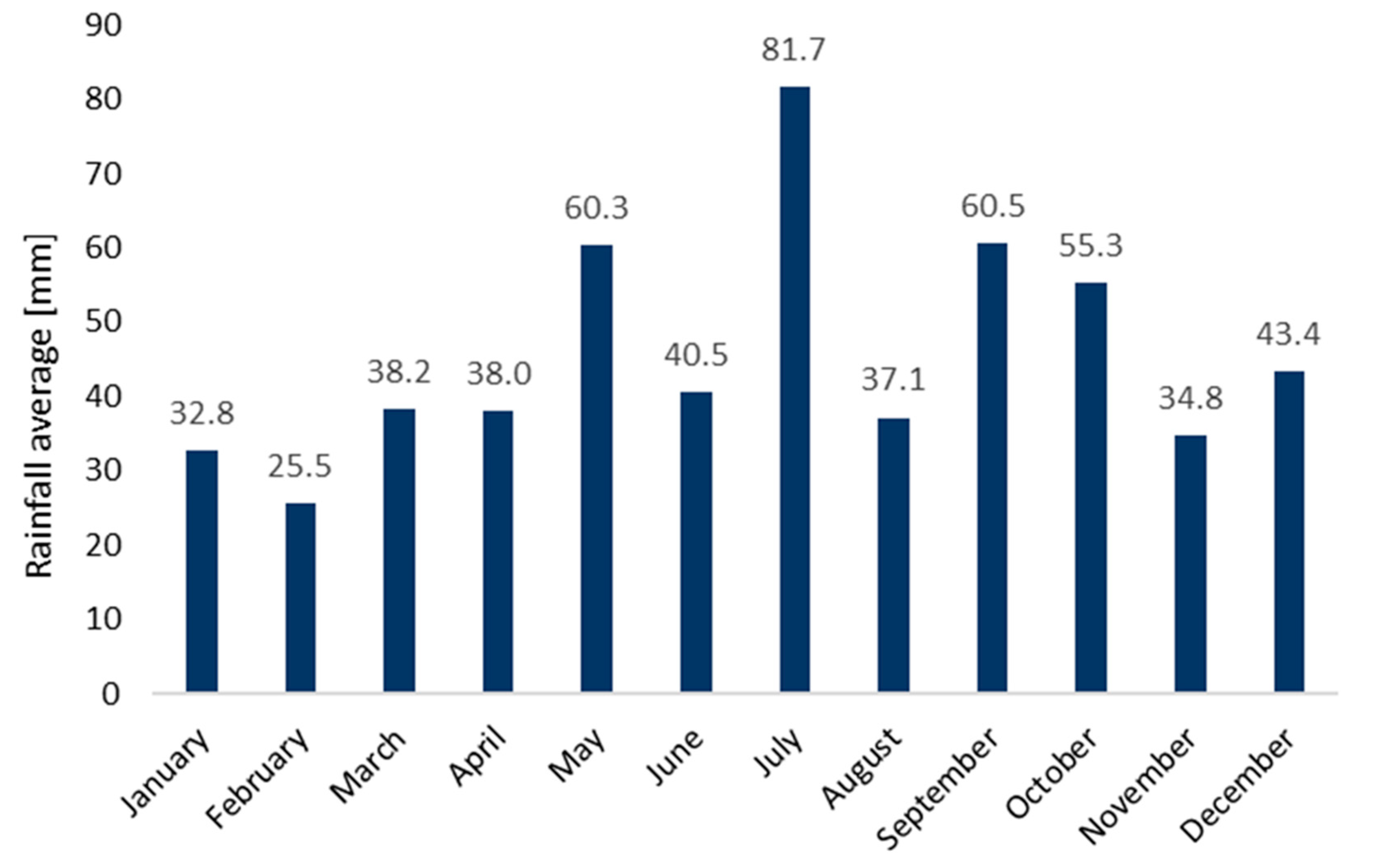
Before preparing the input data, an analysis of precipitation distribution was performed for the study area, based on meteorological data. Data on the sum of monthly precipitation used in the analysis were obtained from the Bulletins of the Polish Institute of Meteorology and Water Management National Research Institute [39]. It covers two stations located closest to the Bogdanka mine (Lublin and Terespol), shown in the Figure 1b. Figure 2 shows a graph of the average sum of precipitation in each month, covering the studied period. It can be noted that the highest sums of rainfall were recorded in July while the lowest were observed in the winter months. It should be noted, however, that from November to March, a snow cover can occur in this region of Poland; therefore, in early spring, the range of areas with a high groundwater level may be enlarged due to snow melting. In the summer (June–August) and autumn (September–November) periods, cycles of large amounts of rainfall or seasonal drought can occur. Due to the above, it was decided that the best period to perform the analysis is springtime, after the thaw period (April), as the period with the average sum of precipitation allowing for the most objective analysis.

2.3. Identification of Flooding Areas Based on the Optical Satellite Data Analysis

The identification of flooding areas over the area of the Bogdanka Coal Mine, and areas directly adjacent to it, was carried out using multispectral imagery from the Sentinel-2 mission (Level-1C product), downloaded from [40]. For research purposes, 9 data packages were obtained in *SAFE format, which contained images showing the reflectance value in 13 spectral channels (from visible light to mid-infrared wavelengths). The aforementioned data set covered images registered over 6-month periods, starting from the second half of the year 2015. In order to increase the accuracy of the conducted analysis, during the selection of data, only images with a cloud cover not exceeding 10% were chosen.
The acquired images were subjected to procedures aimed at standardizing the data registered in various weather and lighting conditions. The first stage consisted of converting the radiometric values of Digital Number (DN) to the value of recorded radiance LSAT according to the following Equation (1):
L S A T = c 0 + c 1 · D N
where c 0 and c 1 are the calibration constants for a given type of sensor and spectra channel, called shift and gain, respectively [41].
The influence of phenomena and processes happening in the atmosphere was reduced in the process of atmospheric correction, during which the following parameters were taken into account: average terrain height (200 m), the aerosol model (in the analyzed case, a model dedicated to poorly urbanized and slightly industrialized areas was adopted [42]) and the atmosphere model (depending on the date of image registration, the models Mid-Latitude Summer, Mid-Latitude Winter and Sub-Arctic Summer were chosen).
During the last stage of pre-processing, the spatial resolution of the data registered in near- and mid-infrared channels was resampled to 10 m (channels 5, 6, 7, 8a, 11 and 12 have a spatial resolution of 20 m) using the bilinear interpolation method.
In order to determine areas of flooding in the study area, two spectral indices were used: Normalized Difference Vegetation Index (NDVI) and Modified Normalized Difference Water Index (MNDWI). The NDVI index was used to identify sites of vegetation degradation. Terrain subsidence, with relatively high groundwater level, may lead to local flooding, having a significant impact on the plant cover condition. The MNDWI index, on the other hand, is a combination of green and mid-infrared channels and was used for the purpose of monitoring changes in the coastlines of water reservoirs (MNDWI assigns positive values to surface waters and negative values to vegetation cover, soil and built-up areas). Table 2 contains the equations used to calculate the spectral indices.
Calculations were carried out in the ENVI 5.5 software, using the following modules: Raster Management, FLAASH, Radiometric Calibration and Band Math.
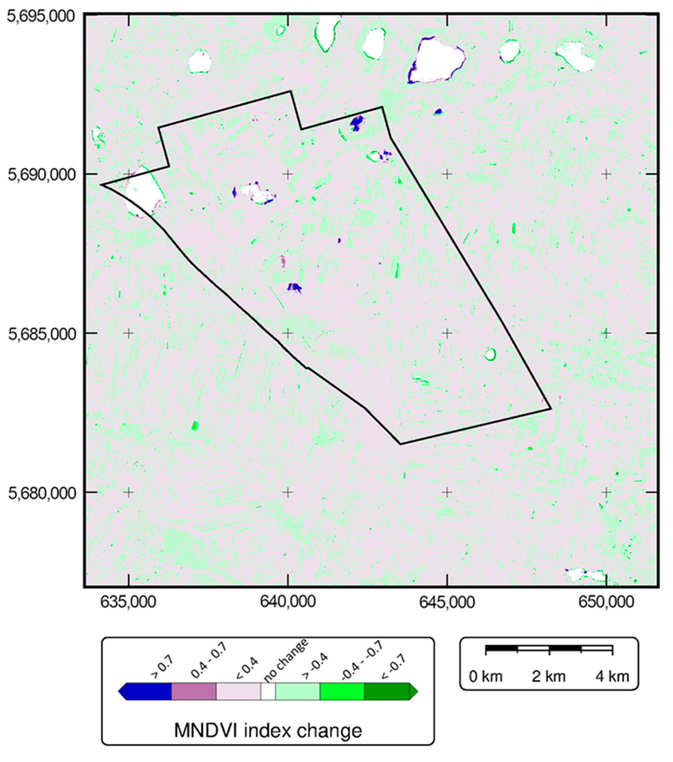
The location of the floodplains was determined on the basis of classification of the image representing the difference between the MNDWI index values for 2015 and 2019. During the process of classification, it was assumed that a change in the said index by a value exceeding 0.9 indicates a significant increase in the area of floodplains or an increase in the area of water reservoirs in the study area. On the other hand, areas where pixels take values between 0.7 and 0.9 may potentially be flooded by groundwater in the future. Figure 3 presents the identified flooding areas within and adjacent to the Bogdanka hard coal mine.
As the results indicate, the floodplains constitute 0.14% of the total area (4597 out of 3,243,601 pixels were classified as floodplains), covering 4511 km2, and are located mostly along the borders of water bodies located in the northern part of the study area. It should be emphasized that the southernmost subdivision zone is located within the area of pseudo-vertical displacements of terrain, the extent of which was determined using Synthetic Aperture Radar Interferometry (InSAR).
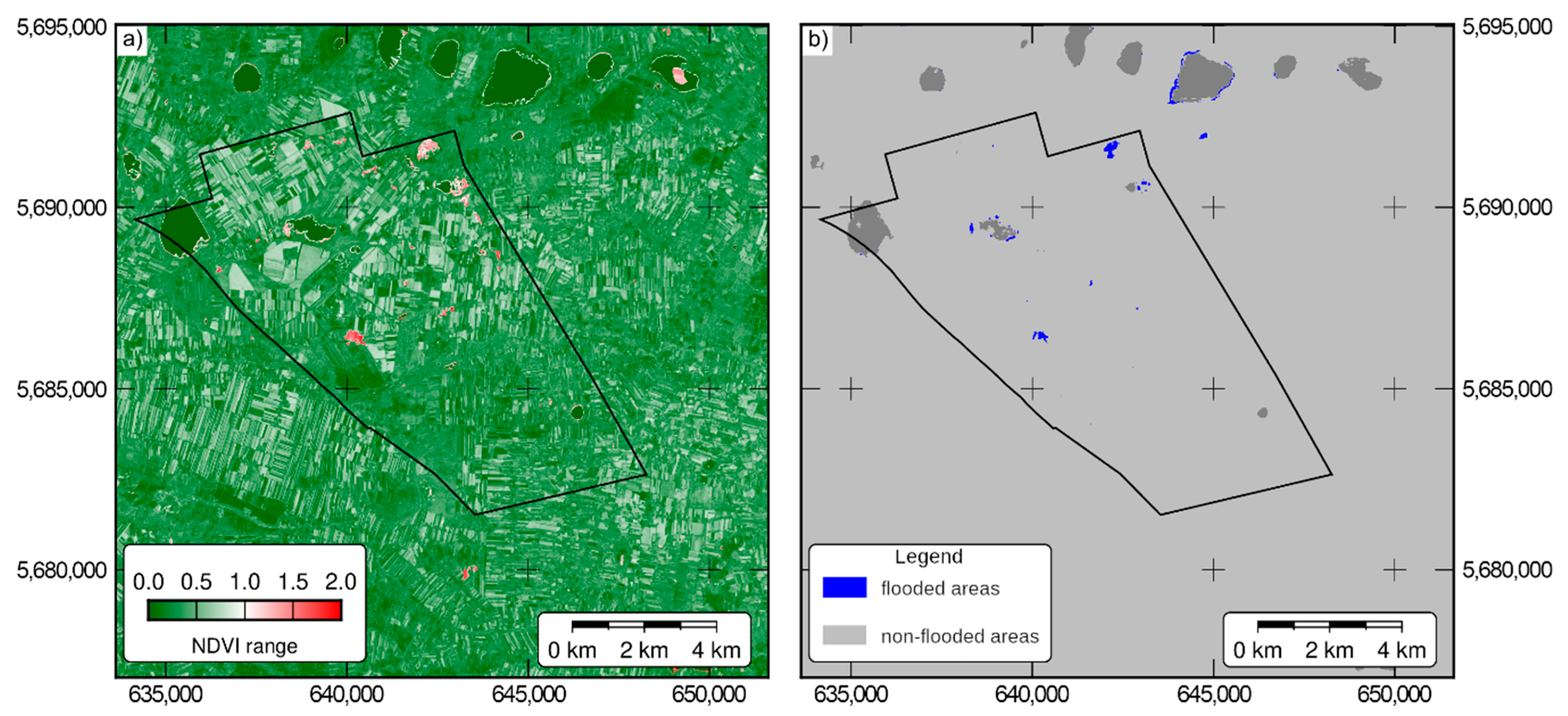
The identification of the flooding zones was also based on the analysis of changes in the NDVI in 2015 and 2019. Figure 4a shows the areas of the smallest and the largest changes in the NDVI in the analyzed time period, and Figure 4b shows the final boundaries of the flooding zones (the zones are located in the places of the largest negative changes in NDVI and the largest positive changes in MNDWI). These areas were used at a later stage in the analyses as input data in the spatial regression model and machine learning.

2.4. InSAR Terrain Displacement Data

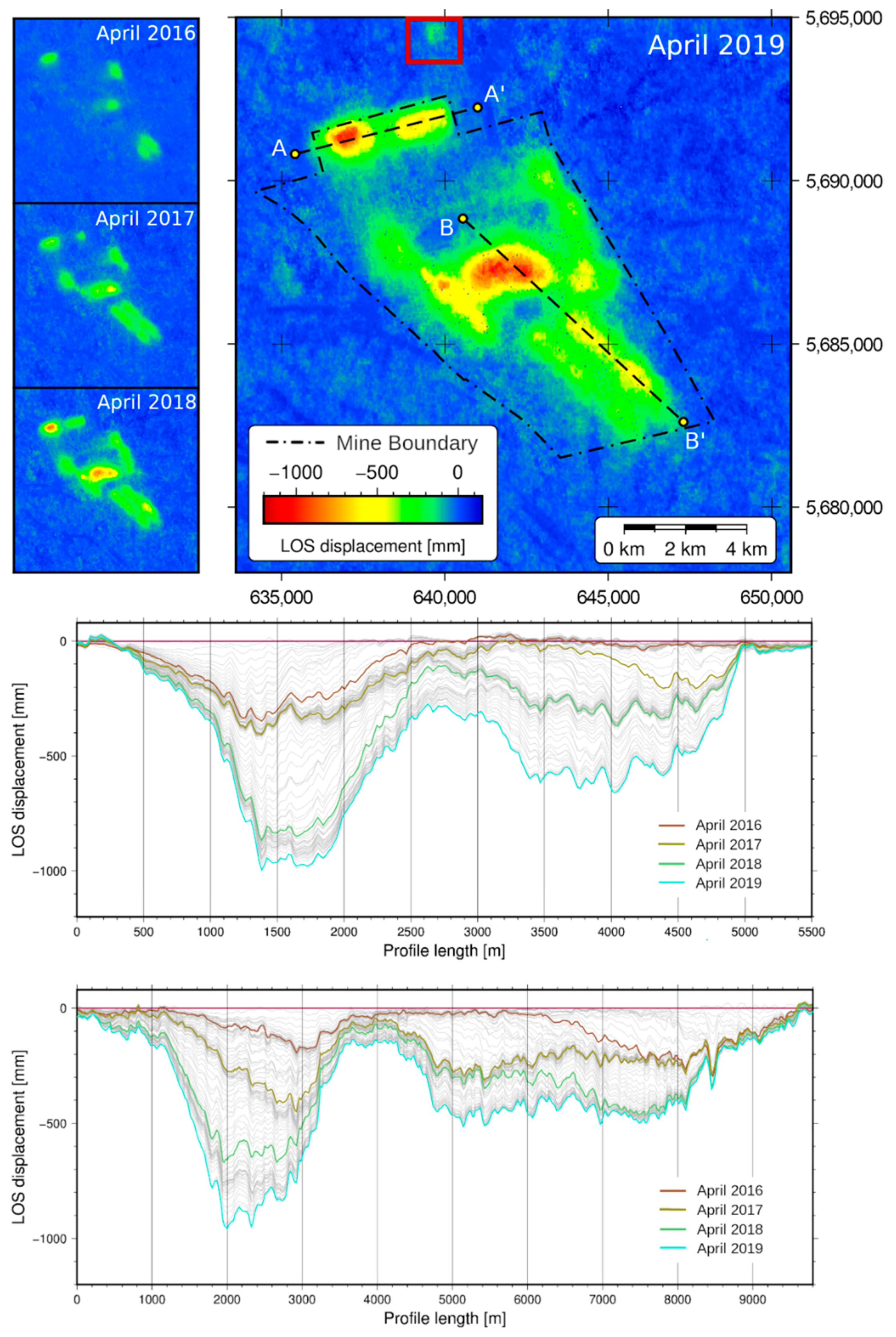
Pseudo-vertical (in the Line of Sight LOS direction) displacements of the terrain caused by underground hard coal mining in the area of the “Bogdanka” mine were determined using Sentinel-1 A/B Synthetic Aperture Radar imagery. The displacement calculations were carried out using the Small Baseline Subset (SBAS) technique [45,46,47], allowing for the processing of interferograms in a time-series manner. A total of 228 SAR images from ascending path no. 131 were used, covering a time period between 26th October 2014 and 1st October 2019. The computational process was performed with the use of the GMTSAR software [48]. The precise orbit ephemerides provided by the Sentinel-1 Quality Control Subsystem [49] were used to correct the satellite state vector. The 1 arc second digital elevation model developed as part of the Shuttle Radar Topography Mission (SRTM) was used to correct for the topographic phase of interferograms [50]. The interferometric phase unwrapping process was carried out using the Statistical-cost Network-flow Algorithm for Phase Unwrapping (SNAPHU) [51,52,53]. A total of 778 interferograms were created for the time-series analysis with the SBAS technique. The results of the SBAS analysis are contained in raster format with cumulative terrain displacements for the date of each acquisition, beginning with the first acquisition (displacement value 0). For further analysis, rasters representing the annual (consistent with optical data) increase in subsidence were selected, i.e., October 2015, April 2016, April 2017, April 2018 and April 2019.
The majority of the subsidence areas were identified in the vicinity of the exploited deposit Bogdanka. Figure 5 shows cumulative displacements from 27 September 2015 to 21 April 2019. The only area outside the deposit boundaries is the Brzezno Lake Reserve, which is located 2 km north of the Bogdanka deposit. Cumulative displacements in this area have reached a maximum of 185 mm. The largest displacements were recorded in the area of the main exploitation field, especially in its northern and central parts, where the cumulative value of terrain displacement has reached up to 1050 mm. Within the other two fields (Stefanów and Nadrybie), the maximum displacement was 600 mm.

2.5. Geological and Hydrogeological Data

The Detailed Geological Map of Poland 1:50,000 and the Hydrogeological Map of Poland—the First Aquifer—Occurrence and Hydrodynamics 1:50,000, provided by the Polish Geological Institute—National Research Institute—were used to select places where, from both geological and engineering standpoints, flooding may occur. The analyzed area of the Bogdanka deposit is contained on four sheets of the above-mentioned maps, numbered 714 (Ostrów Lubelski) [54,55], 715 (Orzechów Nowy) [56,57], 750 (Łęczna) [58,59] and 751 (Siedliszcze) [60,61].
According to the Polish Hydrogeological Dictionary [62], a flooding is defined as “the appearance of groundwater close to the ground surface in connection with: lowering of the ground surface, accumulation of groundwater due to the rising of the water table in watercourses and surface reservoirs, and anthropogenic inhibition of groundwater flow”. The phenomenon of terrain flooding may occur naturally, inter alia in non-drainage depressions, provided there is a poorly permeable substrate below the aquifer or could be a consequence of human activity, especially in the case of underground mining, which leads to the formation of subsidence troughs. Flooding often occurs in large areas with a slight slope or depression, with shallow occurrence of groundwater, in the presence of impermeable or poorly permeable soil, and during the occurrence of heavy rainfall, which lead to an increase in the groundwater level [63].
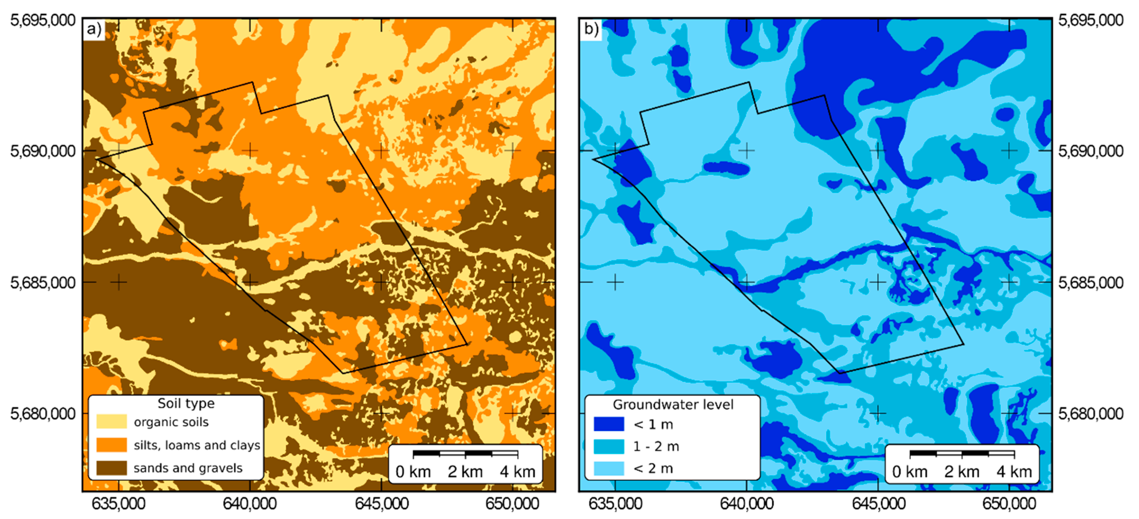
Various sites were classified as areas predisposed to the occurrence of flooding and wetlands— mainly areas with organic soil, originating primarily from lake accumulation, such as low peats (characterized by slowly flowing groundwater), transitional peats (fed mainly with rainwater) and silt, as well as the accompanying clays and stagnant silts and their derivatives, with the simultaneous presence of the groundwater table at a shallow depth (up to 2 m below the terrain level). The obtained data were vectorized to enable their further processing and the classification was performed based on the susceptibility to flooding and occurrence of wetlands. Three categories for the occurrence of the first level of the groundwater table were adopted (Figure 6b):
  • Up to 1 m below ground level.
  • Between 1–2m below ground level.
  • More than 2 m below ground level.
Furthermore, three simplified soil categories were adopted (Figure 6a):
  • Organic soils.
  • Poorly permeable silts, loams and clays.
  • Permeable sands and gravels.

3. Methods—GIS and Machine Learning Analysis

Figure 7 contains a diagram presenting the methodology of data processing and the performed analysis. The individual stages are described in this chapter.

3.1. Overview

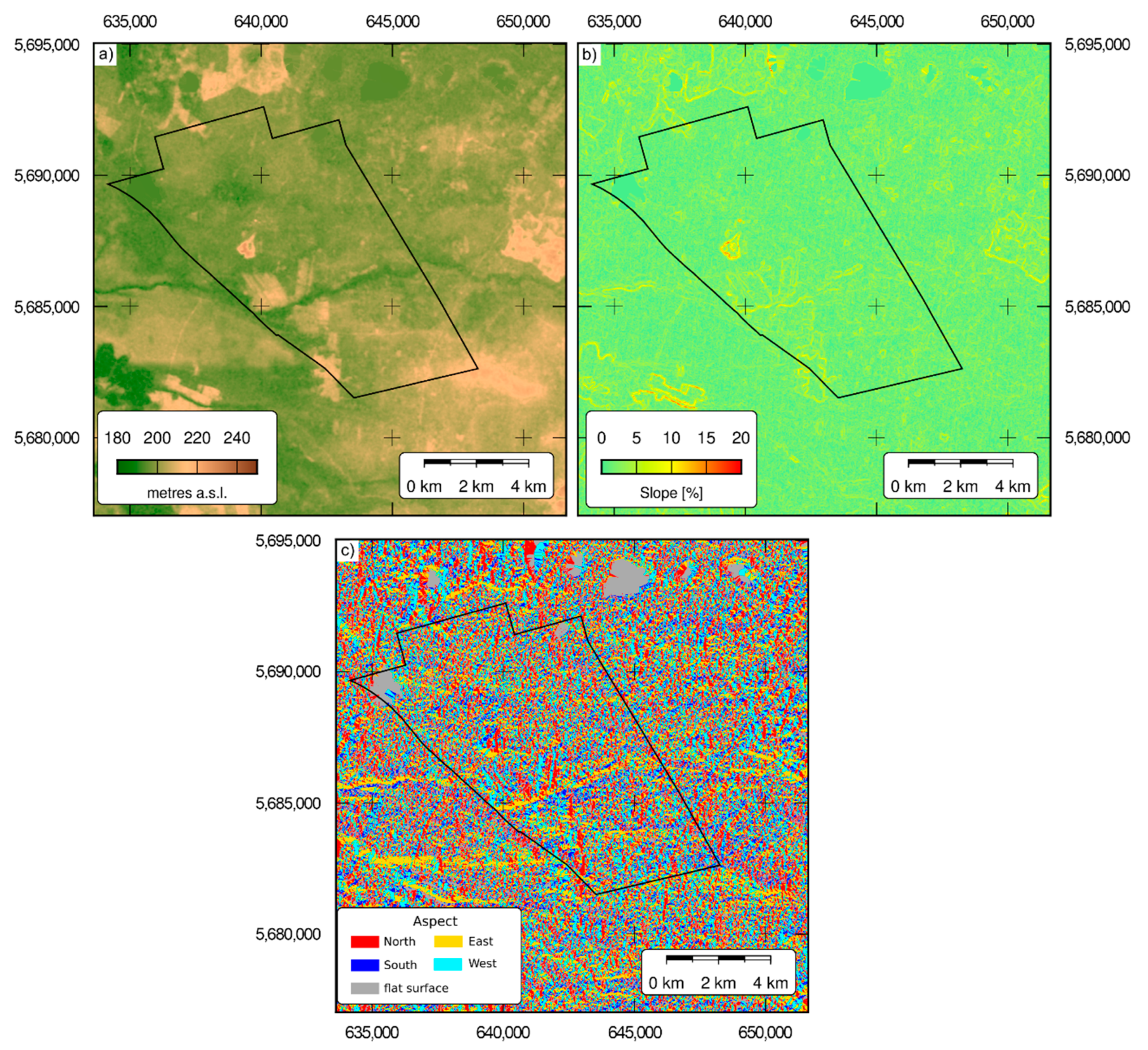
Analysis of the flooding characteristics within the study area started with the preparation of input data. In addition to all the data mentioned in the previous section, a digital elevation model from the SRTM mission was obtained (Figure 8a) [50]. As a result of processing, the rasters of terrain slope (values in %) and exposure (values generalized to 4 main geographical directions and flat terrain) were also obtained (Figure 8b,c, respectively). The above data, as well as the previously developed rasters (Table 3), were combined into a stack of data in a uniform reference frame, spatial extent and spatial resolution. All rasters were transformed into the Universal Transverse Mercator (UTM) reference frame (UTM zone 32N). Data with a spatial resolution other than 10 × 10 m (highest resolution of the Sentinel-2 data) were converted to that resolution using a linear interpolation method. During the analysis, the pixels that did not have correct values for at least one of the rasters were omitted. The range of the NDVI values in the analyzed period were also calculated out of 4 NDVI datasets; for each pixel, a minimum value was subtracted from the maximum. The cumulative terrain displacements for the entire period of the study were calculated as well. Both data pre-processing and proper data analysis and modeling were performed in the Python environment using open-source libraries: numpy [64], sklearn [65], geopandas [66] and pysal [67].

3.2. Preliminary Statistical Analysis

The analysis started with a correlation study between spatial variables that have the potential for being the descriptive variables for the occurrence of flooding. Histograms of independent variable distributions were then prepared and examined. The variable distributions were compared with histograms of variables, separated according to the classification of the flooding areas performed in Section 2.3. Zone statistics describing these distributions were also calculated. This allowed for the selection of factors that may affect the occurrence of flooding and the size of their impact on floodplain formation.

3.3. Machine Learning Global Model

The rate of influence of the examined variables on the occurrence of wetlands was assessed on the basis of a model created with the use of supervised classification. Due to the presence of both continuous and discrete (categorical) variables, the ensemble model based on tree architecture, Random Forest (RF), was selected [68]. After discarding pixels with missing data, 3,177,834 pixels out of the initial 3,243,601 pixels were processed. Incorrect values, which were excluded from the analysis, constituted 2.03% of the total image pixel count. Each pixel contained information about the values of 7 independent variables (features 1–7 in Table 3) and 1 dependent variable (feature 8 in Table 3). The optimal parameters of the RF model, in particular the maximum tree depth, the minimum number of observations in a leaf, the minimum number of observations for branch split and the number of base estimators, were all determined using Grid Search analysis using stratified 3-fold cross-validation. The F1 (4) value, i.e., the harmonic mean of the precision (2) and recall (3) metrics, was selected as a criterion of the quality of the model fit.
p r e c i s i o n = T P T P + F P
r e c a l l = T P T P + F N ,
F 1 = 2 1 p r e c i s i o n + 1 r e c a l l ,
As the RF model is based on an ensemble of decision trees, it is impossible to determine the rate of influence of individual independent variables on the model result, contrary to traditional regression models. It is, however, possible to do so indirectly by analyzing the SHapley Additive exPlanations (SHAP) values. SHAP is based on assumptions resulting from the game theory and allows for the assessment of the size and type of influence of individual explanatory variables on the result of any machine learning or deep learning model [69]. Efficient algorithms are available to calculate SHAP values, in particular for tree-based models [70]. For the RF model used in the analysis, the SHAP values were calculated and analyzed in two ways: (1) the SHAP point values of all observations were summarized, reflecting the positive or negative impact of a given independent variable on the classification of a given pixel as a flooded area and (2) the SHAP values were averaged to obtain the overall weight of a given independent variable in the model’s decision on whether to classify the area as flooded.

3.4. Geographically Weighted Regression (GWR) Local Modeling

The RF model constructed in Section 3.3 is a global model, i.e., it does not take into account the spatial relationships between pixels closely related to each other. In order to check whether such relationships exist, and, as a result, whether the influence of a given explanatory variable on the occurrence of flooding in some regions is greater or smaller than in others, the Geographically Weighted Regression (GWR) model [71] was fitted to the set of explanatory variables with a continuous distribution. This method is based on fitting local regression models to the groupings of observations in a specific neighborhood of each point and can be expressed as (5). Observation weights are determined based on the distance from the central point of a given local regression model (fixed bandwidth) or by the neighborhood rank of the k-nearest neighbors, computed for the central point (adaptive bandwidth).
y i = β 0 ( u i , v i ) + j = 1 r β j ( u i , v i ) x i j + ε i ,   i = 1 ,   2 ,   ,   n
where: yi—values of the dependent variable; xij — independent variables; ui, vi—coordinates of n observations’ locations; β j ( u i , v i ) r + 1 coefficients of the local regression model; ε i —independent, random errors following the N(0, 1) distribution.
The use of GWR allows for the identification and correct modeling of the relationship between the independent variables and the dependent variables in areas where this relationship differs significantly from the global trend. GWR comes in several variants, depending on the type of distribution of dependent variables. Three types of distributions can be used: Gaussian, Poisson and binomial distribution [72]. Due to lack of possibility of simultaneous modeling of variables with different distributions in the utilized software, the GWR model was adjusted only to continuous variables: NDVI range, terrain height, cumulative terrain displacements and slope. During the analysis in Section 4.2, these variables were ranked first, second, fourth and fifth, respectively, in order of the magnitude of the impact on the RF model classification score, so the resulting GWR model should describe the relationships between the variables well enough to identify possible local anomalies in the impact of specific factors. Due to the use of the Gaussian kernel, the analyzed variables were transformed using the Yeo–Johnson power transform [73], converting the distributions of these variables to the standard normal distribution N(0, 1).
Due to computational limitations and a significant excess of data on non-flooded areas, the GWR analysis was carried out on down-sampled data: all pixels with flooding were selected, and an additional 10 times more pixels, selected randomly from the whole study area, were added, representing places of no flooding. The optimal bandwidth of the model was determined by optimizing the Akaike Information Criterion with a correction for small sample sizes (AICc) estimator, which describes the quality of the statistical model used for the comparative analysis of a number of models [72]. Lower estimator values correspond to a higher quality of the model.

4. Results and Discussion

The presentation of analysis results has been divided into three subsections corresponding to the order of operations performed (see Section 3).

4.1. Preliminary Statistical Analysis

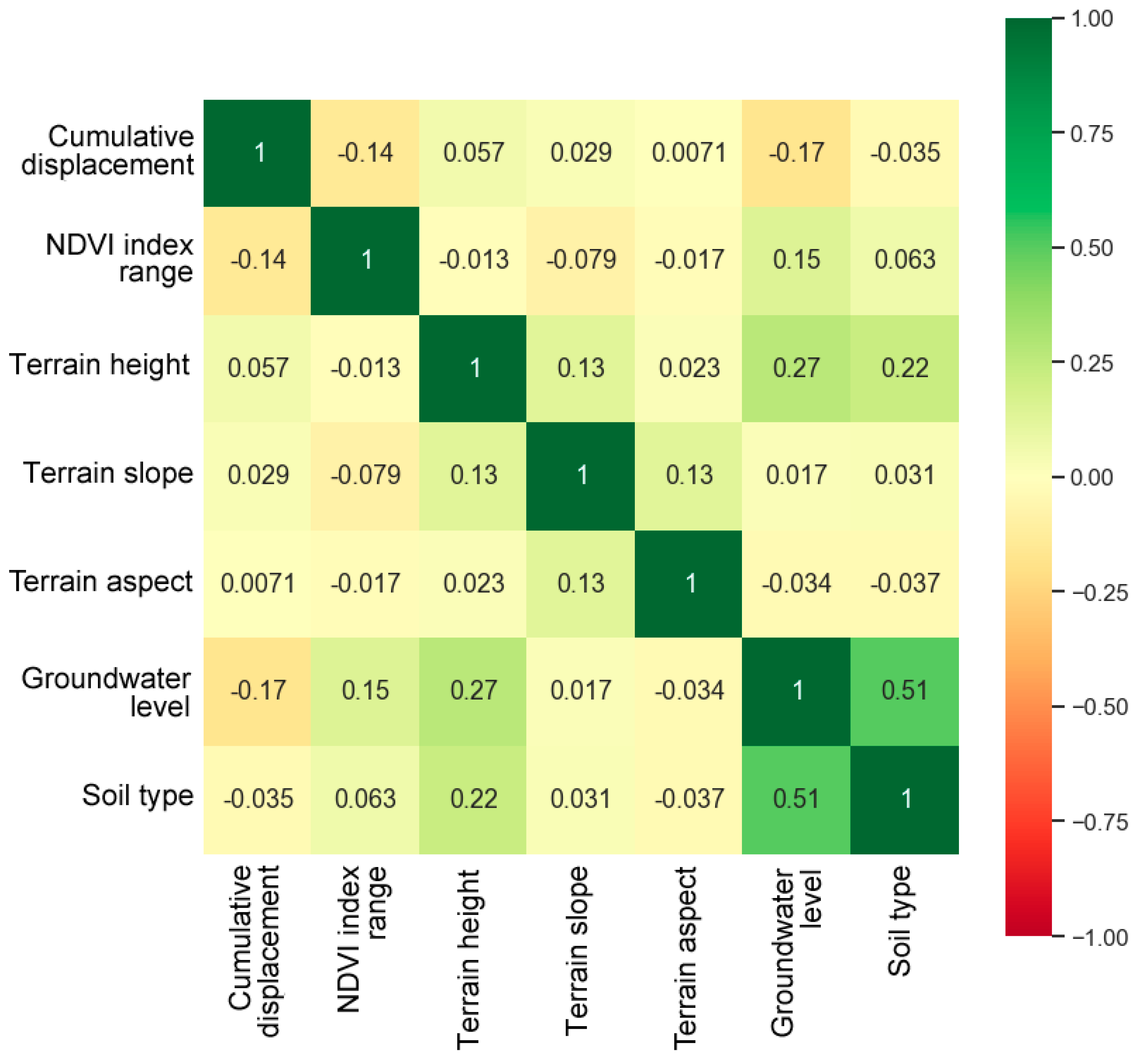
The correlation analysis between spatial variables showed that most of the variables do not have a significant correlation with each other (Figure 9). Only the groundwater depth shows a noticeable correlation with the geological type of the substrate. However, it is not significant enough to consider them as directly dependent (collinearity) and exclude any of them from further analysis.
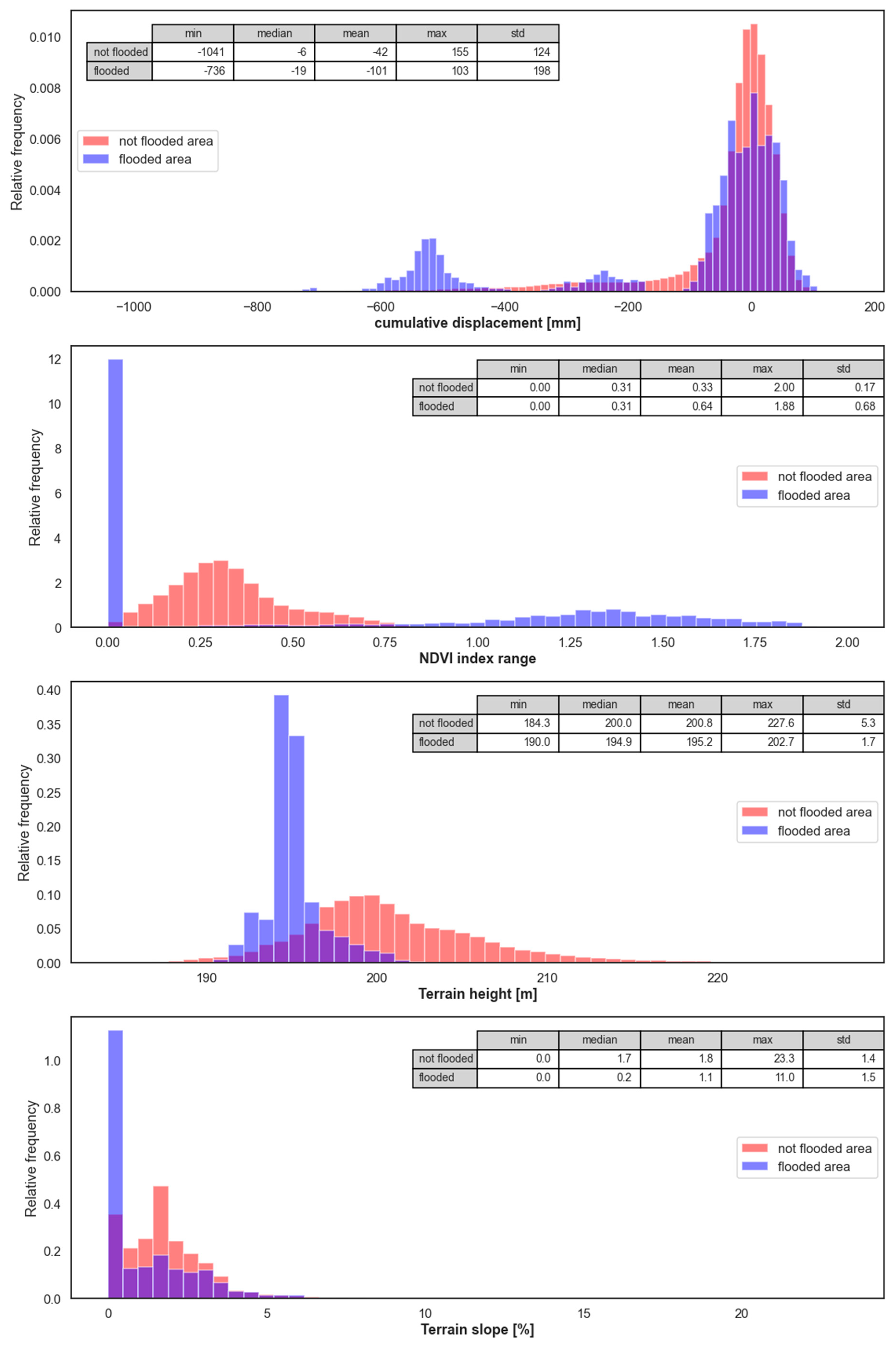
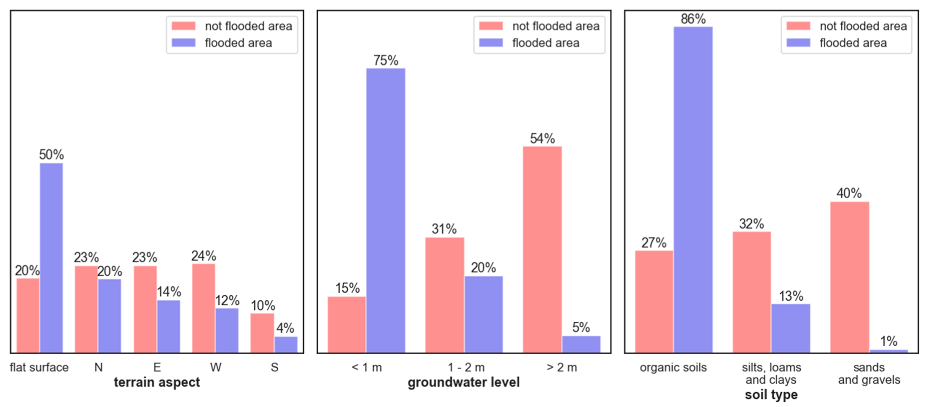
Figure 10 shows histograms and statistics of cumulative displacements, NDVI range, elevation and slope, classified into flooded and non-flooded areas. Results of the same classification of parameters with discrete values: terrain aspect, groundwater level and soil type, are shown in Figure 11.
The histogram of cumulative terrain displacements clearly shows that in the analyzed period, flooding occurred more frequently in the areas of subsidence caused by mining workings. Both mean and median value of subsidence in flooded areas is 2.5–3 times higher than in the rest of the area.
The NDVI index range distribution also indicates differences between flooded areas and areas with no flooding. However, this dependence is not so clear—although, flooding was much more frequent in areas where the NDVI value was approximately constant (and therefore the maximum differences oscillated around 0). The non-flooded areas were most often characterized by moderate differences, reaching 0.3. In the flooded areas, there were maximum NDVI range values, from predominant values of around 0 to very significant differences in the index values, constituting the second distribution mode of around 1.35. Both distribution medians are approximately the same, but their mean values are significantly different: for flooded areas, the mean is almost twice the mean for the remaining areas.
The terrain elevation and the slope histograms clearly show that the flooding occurred mainly in the areas situated relatively low and with low slopes, particularly in flat areas. The mean elevation of the flooded areas was approximately 5 m lower than in other areas. For the slope, the analogous difference in mean values was 0.7%, but their medians differed by more than 1.5%.
The terrain aspect, apart from the more frequent occurrence of flooding in flat areas, already mentioned in the slope analysis, does not show a significantly strong correlation with flooding occurrence. The share of individual geographic directions of exposure for flooded areas, after considering the increase in the share of flat areas, is approximately reduced relative to non-flooded regions. The smallest difference is for areas facing north.
The groundwater level category distributions for flooded and other areas differ substantially. Around 75% of the flooding occurred in areas with the shallowest groundwater table. The regions with the deepest groundwaters account for only 5% of the floodplains, compared to 53% of the entire region where these waters occur. Similarly, the dependence of the geological type of substrate on flooding occurrence is considerable—in the areas most susceptible to water retention, constituting a total of 28% of the study area, 86% of flooding occurred. On the other hand, soil types with the lowest retention, covering 40% of the research area, were covered by only 1% of all flooding.

4.2. Machine Learning Global Model

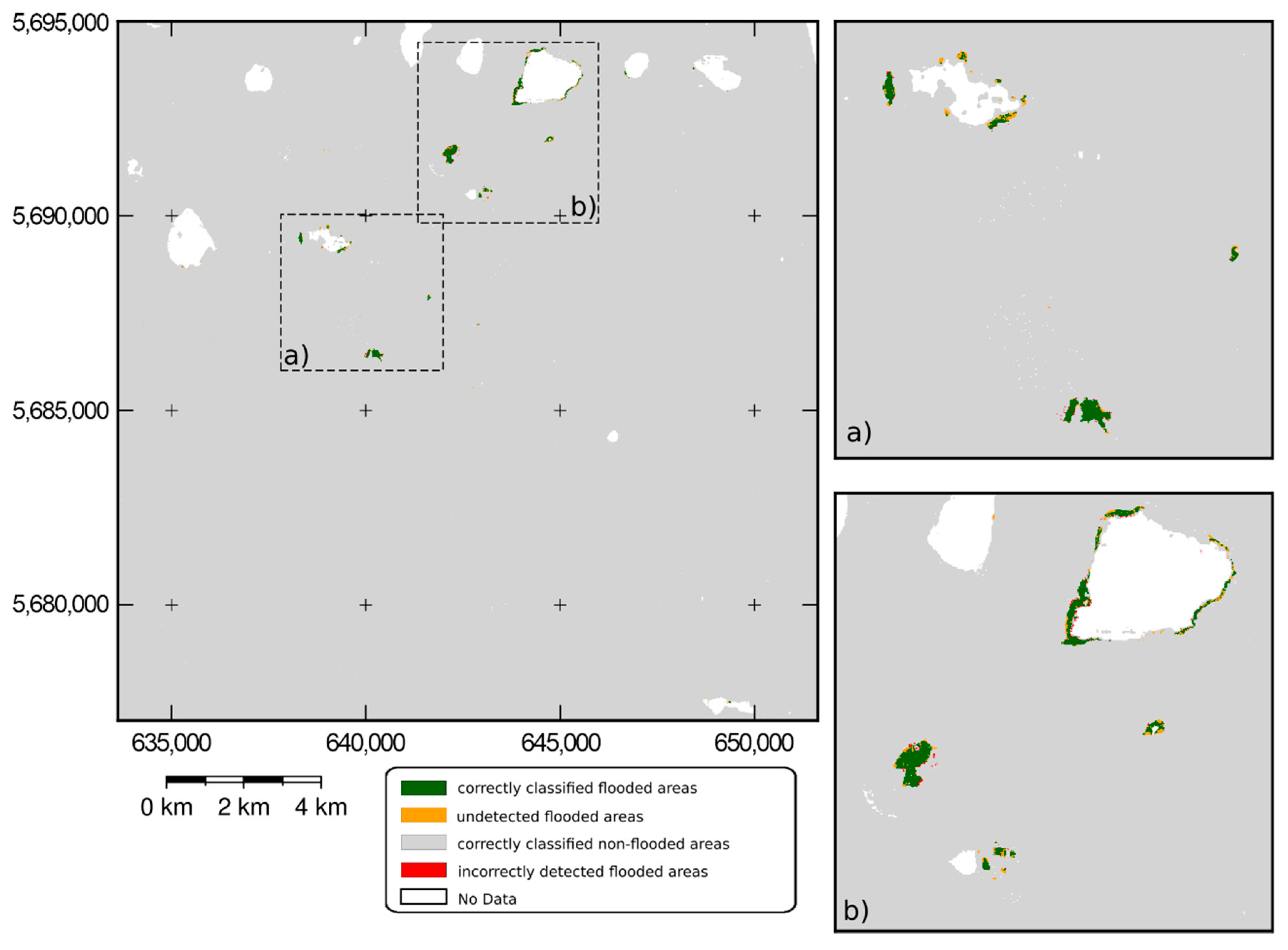
The metrics values of the trained RF model are summarized in Table 4. The confusion matrix is presented in Table 5. The map (Figure 12) depicts the predictions made by the model. It can be seen that the model achieves satisfactory results. The developed RF model correctly detected about 76% of all floodplains, with a total model accuracy of 99.96%. However, it should be considered that pixels classified as flooded are also subject to an error of earlier classification with the MNDWI. Moreover, the discrepancies in the classification results and the RF model’s prediction do not concern most of the entire floodplains but only the spatial extent of individual larger flooding areas, which is visible on the map in Figure 12a,b.
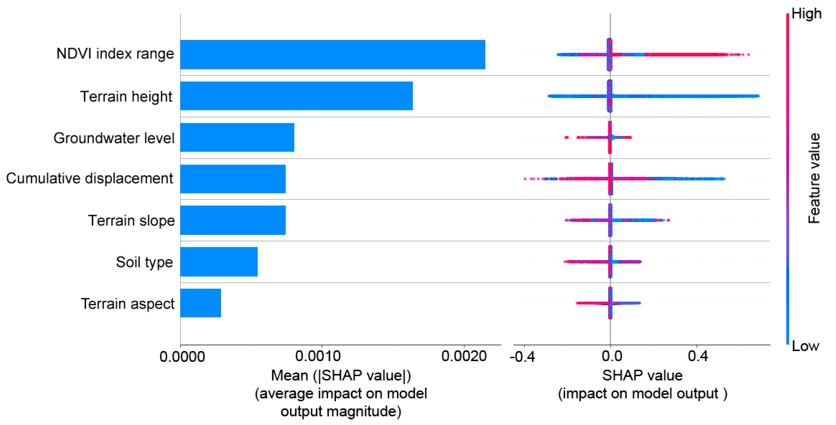
The SHAP values and the averaged influence of the dependent variables are shown in Figure 13. The SHAP values analysis confirms most of the observations made in the histogram analysis in Section 4.1. It accounts for an additional validation of the correct functioning of the developed RF model. High values of the NDVI ranges contributed significantly to the classification of the area as flooded, while low ranges were only of slight importance in reducing the probability of such classification. Lower elevation values contributed to the classification of the area as flooded more often, but it is also clear that many low-lying areas were not classified correctly. High groundwater depth values clearly reduced the likelihood of the site being identified as a floodplain. Large values of subsidence significantly increased this probability, while values around 0 resulted in a slight decrease of possibility of classifying an area as flooded. Areas with a low slope or flat regions had an increased chance of being classified as a floodplain. Finally, high values of the geological type of substrate (corresponding to the areas with the lowest retention) had a negative impact on positive classification.The averaged influence of the dependent variables shows that the NDVI range variable mostly associated with the occurrence of floodplains. This may be due to both the change in characteristics of the electromagnetic wave reflection in the area mostly covered with water and the degradation of vegetation caused by inundation. The next factor is terrain elevation—logically, the local lower areas are more prone to flooding. The next three variables (groundwater level, cumulative terrain displacement and slope) have a similar effect on prediction results. The geological type of subsoil has a slightly lower impact. Exposure has the lowest impact of all variables—flat areas, more prone to flooding, are already included in the slope variable, and the geographic direction of exposure did not turn out to be related to occurrence of inundation.

4.3. GWR Local Modeling

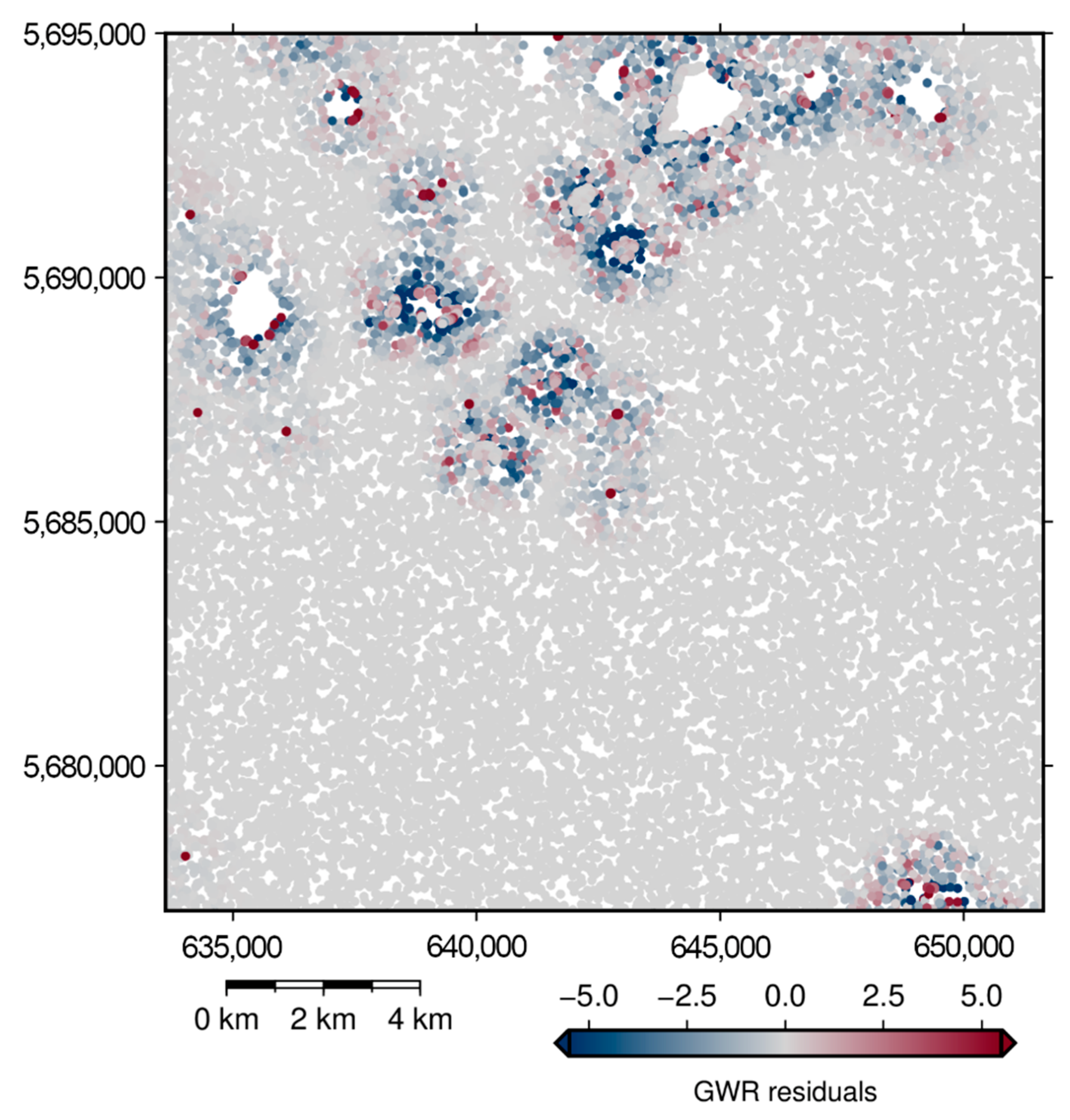
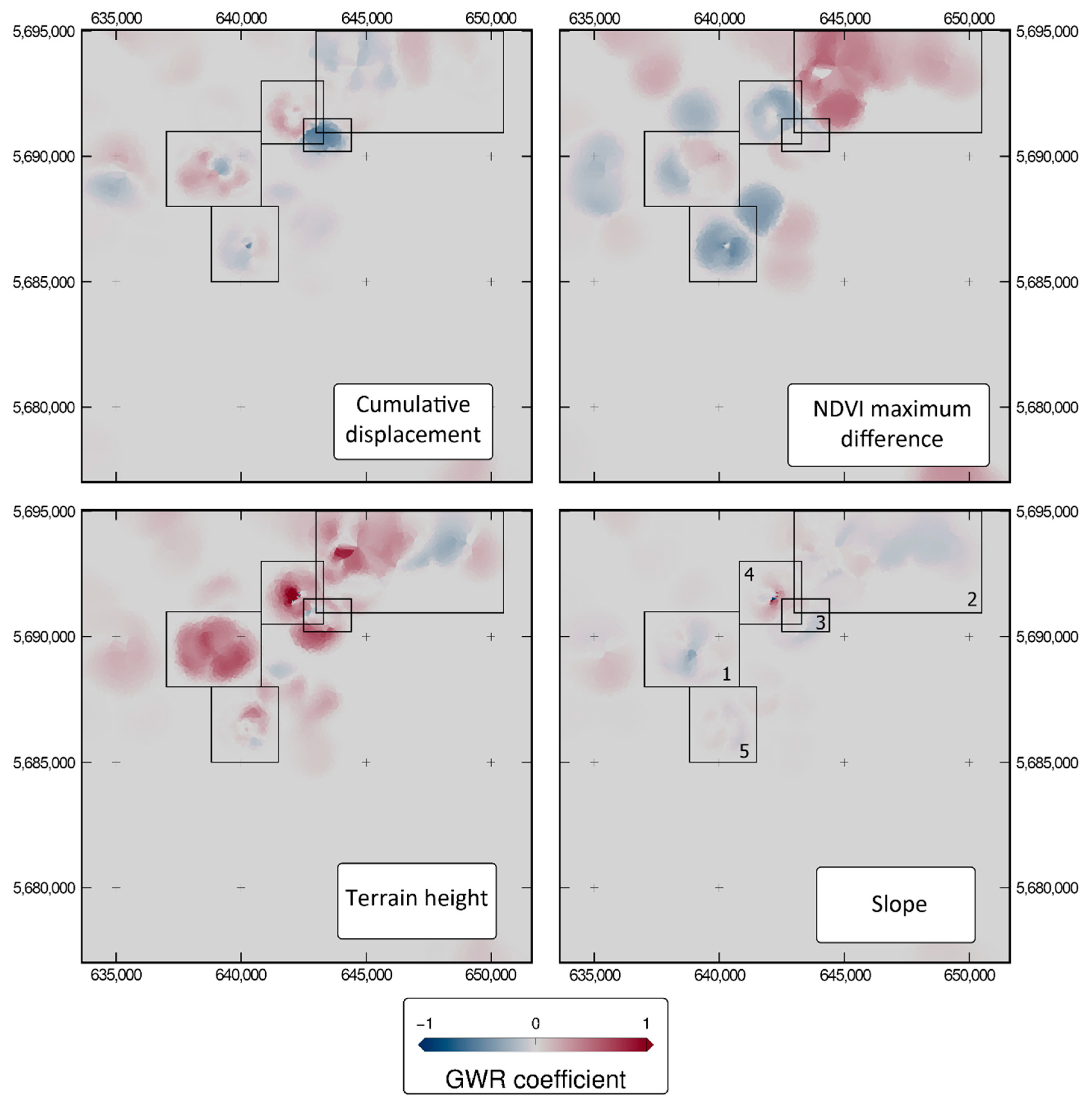
The bandwidth estimated for the optimal AICc value was 383 m. The global linear regression model, fitted to compare the results, has an AICc of 22,533, and the correlation coefficient reaches only 0.02. On its basis, however, the statistical significance of the regionalization of the regression model deviations for a given variable was determined. The GWR model statistics are presented in Table 6. Based on the p-value, for which the statistical significance threshold was set at <5%, it was found that only the relation of flooding and the NDVI range did not show a statistically significant regionalization. The remaining three variables reached p-values below 0.5%. The AICc value for the GWR model was 44,768 and the correlation coefficient was 0.92. This means that the model accounting for the spatial variability of the regression coefficients for the four analyzed dependent variables is much better than the global regression model. The model deviation map (Figure 14) shows a relatively low spatial autocorrelation of positive and negative deviation values—the regionalization of the model prevented the occurrence of large, uniform clusters of similar values of deviation.
The spatial variability of the regression coefficients in the GWR model is shown in Figure 15. Through their analysis, one can see the dependencies causing their regionalization. The areas highlighted in Figure 15 as no. 1, 3 and 4, where the negative values of terrain displacement have a significantly greater impact on the occurrence of flooding, are in fact covering lakes created (or enlarged) as a result of damage caused by mining activities, in particular the subsidence formation and disturbances in local groundwater levels. Negative values of the coefficient for the Z variable are caused by the increased probability of flooding in the subsided regions, but due to local changes in the topography, the magnitude of this impact may be greater or smaller in various regions. For this reason, negative values of the GWR coefficient were obtained in the areas of flooding marked as 1, 3 and 4. In area no. 2, with a topography favoring the occurrence of flooding, there were only a few enlargements of the existing water reservoirs, most likely unrelated to mining activities, hence the positive values of the GWR coefficient for the elevation variable. Based on the NDVI, no significant vegetation degradation was detected in this area, resulting in negative values of this factor assigned in the GWR analysis. The impact of slope on the occurrence of flooding may also vary, depending on the local conditions of the terrain relief, e.g., increasing the risk of flooding in flat areas with natural topography (area no. 1). On the other hand, for the no. 4 area the values of the slope coefficient assume peak values-negative for the area of the water reservoir (because it was formed on a flat area), and positive near its north-west shore, which may be caused by its bigger inclination. In the areas marked with no. 5, flooding has been identified in agricultural areas in the near vicinity of post-mining heaps. NDVI value decreases were also detected for this area, visible on the NDVI range factor map for the GWR method.

4.4. Summary

A very wide spectrum of spatio-temporal data was used in the conducted study: radar and optical imaging from the Sentinel-1 and Sentinel-2 satellites, geological and hydrogeological data and maps, a Digital Elevation Model and meteorological data as well. SBAS satellite radar interferometry and indices based on hyperspectral data as well as GIS tools were used to process these input data. As a result, various datasets (NDVI, LOS displacement time series, groundwater depth, geological substrate, DEM, slope map, aspect map and map of areas identified as flooded, based on the MNDWI index) were used. Based on these datasets, a statistical study of the correlation between spatial variables using spatial regression methods and machine learning supervised classification was performed.
The RF model trained in the study allowed for the correct identification of 76% of flooded zones, based on seven independent spatial variables, and an analysis of the impact of individual variables on the recognition of a given region as susceptible to flooding by the machine learning algorithm. It should also be noted that with the GWR analysis, it was possible to identify and interpret local changes in the magnitude of said impact in selected areas.
Firstly, attention should be paid to the fact that the flooded area formation may be the result of several factors, as is shown by the analysis. Inundations occurred much more frequently in the areas of subsidence caused by mining activities, as well as in natural local sites of terrain depression. An important aspect is that coal mining causes a gradual subsidence of areas where mining is carried out. The process of subsiding is due to the fact that there are no larger geological structures, e.g., faults [74], which would most likely reinforce the terrain deformation process. Over the studied area, the main effect of mining operations is a slow increase in terrain range of the existing subsidence troughs. As the exploitation area grows, the subsiding area also widens. Based on the analysis of cross-sections (Figure 5), it can be concluded that the terrain displacements are not spatially uniform—the change in displacement speed depends on the progress of the front and the exploitation of a given seam. For this reason, in some areas, the rate of subsidence can be very high in one year and can decrease sharply later. Such periodic changes may also affect the rate of appearance and disappearance of floodplains. Contrary to other Polish hard coal mines located in the Silesian region, the influence zone of the Bogdanka mine covers agricultural areas that are not heavily urbanized. Over uninhabited areas, the terrain subsidence causes a seeming rise in the water level [75]. With a relatively high groundwater level in the Bogdanka mine vicinity, its further raising contributes to the enlargement of inundation zones, some of which have a permanent form [76]. This phenomenon is exacerbated by unfavorable weather conditions, such as prolonged rainfall or spring thaw, which may further cause flooding. In places where the variable of cumulative ground displacement is of the greatest significance, primarily water reservoirs and wetlands can be found.
The examples of the use of remote sensing data, GIS and machine learning in the aspect of monitoring changes in the area of terrain surface, quoted in Section 1, do not undertake this issue in such a comprehensive way as the approach adopted in this study. In the presented paper, it was shown that with the combined use of various datasets and modern methods of geospatial data processing and analysis, a more accurate and comprehensive analysis of the occurring phenomena is possible. The methodology presented in the paper can provide a tool for companies from the mining and energy industries to enhance the monitoring of areas affected by mining activities, or by other operations with a significant impact on the surface and the natural environment. Systematic monitoring of the influence of mining on the environment, e.g., the occurrence of flooding, may translate into controlling the degree of weight that underground mining may put on the surface. In line with the idea of sustainable extraction of natural resources, it can play a vital role when mining has a negative social response related to progressing climate changes. Due to the worldwide coverage, as well as open access to the data from the Copernicus Sentinel programme, the adopted methodology can be successfully applied in other areas of raw material extraction. Satellite data mentioned above, as well as geological, hydrological and other data listed in the article, can be extended with additional datasets available for selected areas. An emphasis must be put on the stage of initial data processing and preparation for use with machine learning algorithms and GWR modeling. It should be taken into account, though, that the classification accuracy, as well as the degree of influence of individual factors on the studied phenomenon, may achieve values different from those obtained in this paper, e.g., due to different geological structure and topography, or for particular climate zones and excavation characteristics.

5. Conclusions

An application of various available open-source data (Sentinel-1 SAR imagery, Sentinel-2 optical imagery and other spatial datasets) in monitoring the changes in the natural environment on a case study of an underground coal mine operation was presented in the article. During the study, a focus was put on the area covered by the influence of underground mining operations. Based on the Sentinel-1 SAR data, a Line-of-Sight displacement time-series was calculated using the Small Baseline InSAR technique for the study area, which showed how the terrain surface subsided over the analyzed period (2015–2019). Using Sentinel-2 optical and hyperspectral imagery, the NDVI and MNDWI were calculated, based on which the wetland locations were determined and the overall condition of vegetation was assessed. The derived products of the Sentinel-1 and Sentinel-2 missions, together with data about terrain elevation (DEM), groundwater depth and geological data, were processed using GIS tools and machine learning algorithms. A Random Forest machine learning model was created, which aims at detecting floodplains based on the input data. The developed model achieved an accuracy of about 75%. In addition, a Geographically Weighted Regression (GWR) analysis was conducted on the input data to investigate the influence of individual factors on the occurrence of flooding. The executed analysis showed that the elevation and displacement variables play the most significant role on the probability of wetland occurrence. The GWR analysis also made it possible to identify areas where individual factors may locally influence said probability in a more significant way.
Both the causes and effects of flooding were studied. The results obtained clearly indicate that flooding occurrence does not depend on a single factor but on multiple ones. A significant subsidence of terrain is not the only and the most important factor, as the analysis has shown. Terrain elevation, geological structure of the terrain and groundwater level all play a significant role in the occurrence of flooding. Additionally, the NDVI changes allowed for an assessment of the extent to which flooding affects the condition of the vegetation cover.
In subsequent analyses, it is suggested that more precise geological and hydrogeological data should be used to improve the accuracy of the machine learning model. Furthermore, the model can also be extended with additional variables based on additional meteorological or hydrological geospatial data, which were either not available for the area studied in this paper or their form did not enable their use in spatial modeling.

Author Contributions

Conceptualization, A.K., P.T., D.G., A.B. and K.O.; Methodology, P.T., A.K., A.B. and D.G.; Software, P.T., D.G., A.B.; Validation, A.K., P.T., D.G., A.B. and K.O.; Formal analysis, P.T., D.G. and A.B.; Investigation, P.T., A.B., D.G. and A.K.; Resources, K.O. and M.C.; Data curation, A.B., N.B., P.K., D.G., A.G., P.T. and A.K.; Writing—original draft preparation, A.K., P.T., K.O., N.B., A.B., D.G., M.C. and P.K.; Writing—review and editing, A.K. and D.G.; Visualization, D.G., P.T., A.K., N.B., A.B. and A.G.; Supervision, A.K.; Project administration, A.K. All authors have read and agreed to the published version of the manuscript.

Funding

The research was partly supported by the statutory grant at the Department of Mining and Geodesy, Faculty of Geoengineering, Mining and Geology, Wroclaw University of Science and Technology.

Conflicts of Interest

The authors declare no conflict of interest.

Abbreviations

AICcAkaike Information Criterion with a correction for small sample sizes
CCRCentral Coal Region
DNDigital Number
DEMDigital Elevation Model
GISGeographic Information Systems
GWRGeographically Weighted Regression
InSARInterferometric Synthetic Aperture Radar
LCBLublin Coal Basin
LOSLine of Sight
MNDWIModified Normalized Difference Water Index
NDVINormalized Difference Vegetation Index
RFRandom Forest
SARSynthetic Aperture Radar
SBASSmall Baseline Subset
SHAPSHapley Additive exPlanations
SNAPHUStatistical-cost Network-flow Algorithm for Phase Unwrapping
SRTMShuttle Radar Topography Mission
UTMUniversal Transverse Mercator

References

  1. Klukanová, A.; Rapant, S. Impact of mining activities upon the environment of the Slovak Republic: Two case studies. J. Geochem. Explor. 1999, 66, 299–306. [Google Scholar] [CrossRef]
  2. Chauhan, S.S. Mining, Development and Environment: A Case Study of Bijolia Mining Area in Rajasthan, India. J. Hum. Ecol. 2010, 31, 65–72. [Google Scholar] [CrossRef]
  3. Majumder, S.; Sarkar, K. Impact of mining and related activities on physical and cultural environment of Singrauli Coalfield—A case study through application of remote sensing techniques. J. Indian Soc. Remote Sens. 1994, 22, 45–56. [Google Scholar] [CrossRef]
  4. Nichols, O.G.; Carbon, B.A.; Colquhoun, I.J.; Croton, J.T.; Murray, N.J. Rehabilitation after bauxite mining in south-western australia. Landsc. Plan. 1985, 12, 75–92. [Google Scholar] [CrossRef]
  5. Sklenicka, P.; Prikyl, I. Non-productive principles of landscape rehabilitation after long-term opencast mining in north-west Bohemia. J. S. Afr. Inst. Min. Metall. 2004, 104, 83–88. [Google Scholar]
  6. Lechner, A.M.; Kassulke, O.; Unger, C. Spatial assessment of open cut coal mining progressive rehabilitation to support the monitoring of rehabilitation liabilities. Resour. Policy 2016, 50, 234–243. [Google Scholar] [CrossRef]
  7. Kwinta, A.; Gradka, R. Mining exploitation influence range. Nat. Hazards 2018, 94, 979–997. [Google Scholar] [CrossRef] [Green Version]
  8. Kwinta, A.; Gradka, R. Analysis of the damage influence range generated by underground mining. Int. J. Rock Mech. Min. Sci. 2020, 128, 104263. [Google Scholar] [CrossRef]
  9. Blachowski, J.; Milczarek, W. Analysis of surface changes in the Walbrzych hard coal mining grounds (SW Poland) between 1886 and 2009. Geol. Q. 2014, 58, 353–368. [Google Scholar] [CrossRef] [Green Version]
  10. Blachowski, J.; Kopec, A.; Milczarek, W.; Owczarz, K. Evolution of Secondary Deformations Captured by Satellite Radar Interferometry: Case Study of an Abandoned Coal Basin in SW Poland. Sustainability 2019, 11, 884. [Google Scholar] [CrossRef] [Green Version]
  11. Szczepiński, J. The Significance of Groundwater Flow Modeling Study for Simulation of Opencast Mine Dewatering, Flooding, and the Environmental Impact. Water 2019, 11, 848. [Google Scholar] [CrossRef] [Green Version]
  12. Currell, M.J.; Werner, A.D.; McGrath, C.; Webb, J.A.; Berkman, M. Problems with the application of hydrogeological science to regulation of Australian mining projects: Carmichael Mine and Doongmabulla Springs. J. Hydrol. 2017, 548, 674–682. [Google Scholar] [CrossRef]
  13. Milczarek, W. Investigation of post inducted seismic deformation of the 2016 MW 4.2 Tarnowek Poland mining tremor based on DinSAR and SBAS method. Acta Geodyn. Geomater. 2019, 16, 183–193. [Google Scholar] [CrossRef]
  14. Hejmanowski, R.; Malinowska, A.A.; Witkowski, W.T.; Guzy, A. An Analysis Applying InSAR of Subsidence Caused by Nearby Mining-Induced Earthquakes. Geosciences 2019, 9, 490. [Google Scholar] [CrossRef] [Green Version]
  15. Sonter, L.J.; Moran, C.J.; Barrett, D.J.; Soares-Filho, B.S. Processes of land use change in mining regions. J. Clean. Prod. 2014, 84, 494–501. [Google Scholar] [CrossRef] [Green Version]
  16. Redondo-Vega, J.M.; Gómez-Villar, A.; Santos-González, J.; González-Gutiérrez, R.B.; Álvarez-Martínez, J. Changes in land use due to mining in the north-western mountains of Spain during the previous 50years. Catena 2017, 149, 844–856. [Google Scholar] [CrossRef]
  17. Malinowska, A.; Hejmanowski, R. Building damage risk assessment on mining terrains in Poland with GIS application. Int. J. Rock Mech. Min. Sci. 2010, 47, 238–245. [Google Scholar] [CrossRef]
  18. Florkowska, L. Example building damage caused by mining exploitation in disturbed rock mass. Stud. Geotech. Mech. 2013, 35, 19–37. [Google Scholar] [CrossRef] [Green Version]
  19. Brinson, M.M. A Hydrogeomorphic Classification for Wetlands; U.S. Army Engineer Waterways Experiment Station: Vicksburg, MS, USA, 1993; pp. 1–103. [Google Scholar]
  20. Padmanaban, R.; Bhowmik, A.K.; Cabral, P. A Remote Sensing Approach to Environmental Monitoring in a Reclaimed Mine Area. ISPRS Int. J. Geo-Inf. 2017, 6, 401. [Google Scholar] [CrossRef] [Green Version]
  21. Charou, E.; Stefouli, M.; Dimitrakopoulos, D.; Vasiliou, E.; Mavrantza, O.D. Using Remote Sensing to Assess Impact of Mining Activities on Land and Water Resources. Mine Water Environ. 2010, 29, 45–52. [Google Scholar] [CrossRef]
  22. Paull, D.; Banks, G.; Ballard, C.; Gillieson, D. Monitoring the Environmental Impact of Mining in Remote Locations through Remotely Sensed Data. Geocarto Int. 2006, 21, 33–42. [Google Scholar] [CrossRef]
  23. Miatkowski, Z.; Kowalik, W.; Lewiński, S.; Sołtysik, A.; Turbiak, J. Assessment of Possibilities of Satellite Remote Sensing use for the Identification of Hydrogenic Habitats Transformations under the Influence of Deep Drainage in the Region of the Bełchatów Brown Coal Mine. (In Polish with English summary). Available online: http://warsztatygornicze.pl/wp-content/uploads/2004_36.pdf (accessed on 10 November 2020).
  24. Wang, X.; Nie, H.-F.; Li, C.-Z.; Wang, J. Application of different data sources in the investigation of exploitation situation and environment of mines. Remote Sens. Land Resour. 2006, 68, 69–71. [Google Scholar] [CrossRef]
  25. Schmidt, H.; Glaesser, C. Multitemporal analysis of satellite data and their use in the monitoring of the environmental impacts of open cast lignite mining areas in Eastern Germany. Int. J. Remote Sens. 1998, 19, 2245–2260. [Google Scholar] [CrossRef]
  26. Duan, H.; Deng, Z.; Deng, F.; Wang, D. Assessment of Groundwater Potential Based on Multicriteria Decision Making Model and Decision Tree Algorithms. Available online: https://www.hindawi.com/journals/mpe/2016/2064575/ (accessed on 6 September 2020).
  27. Baek, J.; Kim, S.-W.; Park, H.-J.; Jung, H.-S.; Kim, K.-D.; Kim, J.W. Analysis of ground subsidence in coal mining area using SAR interferometry. Geosci. J. 2008, 12, 277–284. [Google Scholar] [CrossRef]
  28. Zhao, C.; Lu, Z.; Zhang, Q. Time-series deformation monitoring over mining regions with SAR intensity-based offset measurements. Remote Sens. Lett. 2013, 4, 436–445. [Google Scholar] [CrossRef]
  29. Samsonov, S.; D’Oreye, N.; Smets, B. Ground deformation associated with post-mining activity at the French–German border revealed by novel InSAR time series method. Int. J. Appl. Earth Obs. Geoinf. 2013, 23, 142–154. [Google Scholar] [CrossRef]
  30. Gee, D.; Bateson, L.; Sowter, A.; Grebby, S.; Novellino, A.; Cigna, F.; Marsh, S.; Banton, C.; Wyatt, L. Ground Motion in Areas of Abandoned Mining: Application of the Intermittent SBAS (ISBAS) to the Northumberland and Durham Coalfield, UK. Geosciences 2017, 7, 85. [Google Scholar] [CrossRef] [Green Version]
  31. Bateson, L.; Cigna, F.; Boon, D.; Sowter, A. The application of the Intermittent SBAS (ISBAS) InSAR method to the South Wales Coalfield, UK. Int. J. Appl. Earth Obs. Geoinf. 2015, 34, 249–257. [Google Scholar] [CrossRef] [Green Version]
  32. Zhao, Y.; Li, Y.; Zhang, L.; Wang, Q. Groundwater level prediction of landslide based on classification and regression tree. Geodesy Geodyn. 2016, 7, 348–355. [Google Scholar] [CrossRef] [Green Version]
  33. Zhu, X.; Xu, Q.; Tang, M.; Nie, W.; Ma, S.; Xu, Z. Comparison of two optimized machine learning models for predicting displacement of rainfall-induced landslide: A case study in Sichuan Province, China. Eng. Geol. 2017, 218, 213–222. [Google Scholar] [CrossRef]
  34. Karimi, S.S.; Saintilan, N.; Wen, L.; Valavi, R. Application of Machine Learning to Model Wetland Inundation Patterns Across a Large Semiarid Floodplain. Water Resour. Res. 2019, 55, 8765–8778. [Google Scholar] [CrossRef]
  35. Bońda, R.; Brzeziński, D.; Czapigo-Czapla, M.; Czapowski, G.; Fabiańczyk, J.; Kalinowska, A.; Malon, A.; Mazurek, S.; Mikulski, S.Z.; Miśkiewicz, W.; et al. Balance of Mineral Resources in Poland as at 31 December 2019; Polish Geological Institute–National Research Institute: Warsaw, Poland, 2020. [Google Scholar]
  36. Lubelski Coal “Bogdanka” Characteristics of Coal Deposit. 2018. Available online: https://www.lw.com.pl/en,2,s169.html (accessed on 10 September 2020).
  37. Stachowicz, S. Current Problems of Exploitations of Hard Coal in “Bogdanka” Mine in Lublin Coal Basin (LZW). (In Polish with English Summary). Available online: http://warsztatygornicze.pl/wp-content/uploads/2005-1.pdf (accessed on 10 November 2020).
  38. Stupicka, E.; Stempień-Sałek, M. Regional Geology of Poland; University of Warsaw Publishing House: Warsaw, Poland, 2019; pp. 161–168. ISBN 978-83-235-2022-1. (In Polish) [Google Scholar]
  39. Bulletins of the Polish Institute of Meteorology and Water Management; Institute of Meteorology and Water Management–National Research Institute: Warsaw, Poland, 2015.
  40. U.S. Geological Survey, EarthExplorer. Available online: https://earthexplorer.usgs.gov/ (accessed on 15 August 2020).
  41. Osińska-Skotak, K. The Importance of Radiometric Correction in Sarellite Images. Arch. Photogramm. Cartogr. Remote Sens. 2007, 17, 577–590, (In Polish with English summary). [Google Scholar]
  42. Harris Geospatial Solutions, Inc. Fast Line-of-Sight Atmospheric Analysis of Hypercubes (FLAASH). Available online: https://www.l3harrisgeospatial.com/docs/FLAASH.html (accessed on 17 August 2020).
  43. Bell, G.E. Turfgrass Physiology and Ecology: Advanced Management Principles; CABI: Wallingford, UK, 2011; ISBN 978-1-84593-648-8. [Google Scholar]
  44. Acharya, T.D.; Lee, D.H.; Yang, I.T.; Lee, J.K. Identification of Water Bodies in a Landsat 8 OLI Image Using a J48 Decision Tree. Sensors 2016, 16, 1075. [Google Scholar] [CrossRef] [PubMed] [Green Version]
  45. Berardino, P.; Fornaro, G.; Lanari, R.; Sansosti, E. A new algorithm for surface deformation monitoring based on small baseline differential SAR interferograms. IEEE Trans. Geosci. Remote Sens. 2002, 40, 2375–2383. [Google Scholar] [CrossRef] [Green Version]
  46. Schmidt, D.A.; Bürgmann, R. Time-dependent land uplift and subsidence in the Santa Clara valley, California, from a large interferometric synthetic aperture radar data set. J. Geophys. Res. Solid Earth 2003, 108. [Google Scholar] [CrossRef] [Green Version]
  47. Tong, X.; Schmidt, D. Active movement of the Cascade landslide complex in Washington from a coherence-based InSAR time series method. Remote Sens. Environ. 2016, 186, 405–415. [Google Scholar] [CrossRef]
  48. Sandwell, D.T.; Mellors, R.J.; Tong, X.; Wei, M.; Wessel, P. Open radar interferometry software for mapping surface Deformation. Eos Trans. Am. Geophys. Union 2011, 92, 234. [Google Scholar] [CrossRef] [Green Version]
  49. European Space Agency, Sentinel-1 Quality Control. Available online: https://qc.sentinel1.eo.esa.int/ (accessed on 19 February 2020).
  50. Farr, T.G.; Rosen, P.A.; Caro, E.; Crippen, R.; Duren, R.; Hensley, S.; Kobrick, M.; Paller, M.; Rodriguez, E.; Roth, L.; et al. The Shuttle Radar Topography Mission. Rev. Geophys. 2007, 45. [Google Scholar] [CrossRef] [Green Version]
  51. Chen, C.W.; Zebker, H.A. Network approaches to two-dimensional phase unwrapping: Intractability and two new algorithms. J. Opt. Soc. Am. A 2000, 17, 401–414. [Google Scholar] [CrossRef]
  52. Chen, C.W.; Zebker, H.A. Two-dimensional phase unwrapping with use of statistical models for cost functions in nonlinear optimization. J. Opt. Soc. Am. A 2001, 18, 338–351. [Google Scholar] [CrossRef] [Green Version]
  53. Chen, C.W.; Zebker, H.A. Phase unwrapping for large SAR interferograms: Statistical segmentation and generalized network models. IEEE Trans. Geosci. Remote Sens. 2002, 40, 1709–1719. [Google Scholar] [CrossRef] [Green Version]
  54. Liszkowski, J. Detailed Geological Map of Poland 1:50 000, Sheet 714 (Ostrów Lubelski); Polish Geological Institute–National Research Institute: Warsaw, Poland, 1977. [Google Scholar]
  55. Czerwińska-Tomczyk, J.; Łusiak, R. Hydrogeological Map of Poland 1:50 000, First Aquifer, Occurrence and Hydrodynamics, Sheet 714 (Ostrów Lubelski); Polish Geological Institute–National Research Institute: Warsaw, Poland, 2005. [Google Scholar]
  56. Buraczyński, J.; Wojtanowicz, J. Detailed Geological Map of Poland 1:50 000, Sheet 715 (Orzechów Nowy); Polish Geological Institute–National Research Institute: Warsaw, Poland, 1979. [Google Scholar]
  57. Rysak, A.; Zwoliński, Z. Hydrogeological Map of Poland 1:50 000, First Aquifer, Occurrence and Hydrodynamics, Sheet 715 (Orzechów Nowy); Polish Geological Institute–National Research Institute: Warsaw, Poland, 2005. [Google Scholar]
  58. Harasimiuk, M.; Henkiel, A. Detailed Geological Map of Poland 1:50 000, Sheet 750 (Łęczna); Polish Geological Institute–National Research Institute: Warsaw, Poland, 1978. [Google Scholar]
  59. Pietruszka, W.; Zezula, H. Hydrogeological Map of Poland 1:50 000, First Aquifer, Occurrence and Hydrodynamics, Sheet 750 (Łęczna); Polish Geological Institute–National Research Institute: Warsaw, Poland, 2006. [Google Scholar]
  60. Harasimiuk, M.; Szwajgier, W.; Jezierski, W. Detailed Geological Map of Poland 1:50 000, Sheet 751 (Siedliszcze); Polish Geological Institute–National Research Institute: Warsaw, Poland, 1998. [Google Scholar]
  61. Zezula, H.; Pietruszka, W. Hydrogeological Map of Poland 1:50 000, First Aquifer, Occurrence and Hydrodynamics, Sheet 751 (Siedliszcze); Polish Geological Institute–National Research Institute: Warsaw, Poland, 2006. [Google Scholar]
  62. Dowgiałło, J.; Kleczkowski, A.S.; Macioszczyk, T.; Różkowski, A. (Eds.) Hydrogeological Dictionary; Polish Geological Institute–National Research Institute: Warsaw, Poland, 2002. (In Polish) [Google Scholar]
  63. Frankowski, Z.; Gałkowski, P.; Majer, K. Directions of Use Maps of Areas at Risk of Flooding in May 2010; Polish Geological Institute–National Research Institute: Warsaw, Poland. Available online: https://www.pgi.gov.pl/psh/materialy-informacyjne-psh/artykuly-psh/8851-artykul-2010-kierunki-wykorzystania-mapy-obszarow-zagrozonych-ryzykiem-podtopien-w-majowej-powodzi-2010-roku.html (accessed on 17 August 2020).
  64. Oliphant, T.E. A Guide to NumPy; Trelgol Publishing: USA, 2006; Volume 1. Available online: https://numpy.org/ (accessed on 25 August 2020).
  65. Pedregosa, F.; Varoquaux, G.; Gramfort, A.; Michel, V.; Thirion, B.; Grisel, O.; Blondel, M.; Prettenhofer, P.; Weiss, R.; Dubourg, V.; et al. Scikit-learn: Machine learning in Python. J. Mach. Learn. Res. 2011, 12, 2825–2830. [Google Scholar]
  66. Jordahl, K. GeoPandas: Python Tools for Geographic Data. 2014. Available online: https://github.com/geopandas/geopandas (accessed on 25 August 2020).
  67. Rey, S.J.; Anselin, L. PySAL: A Python Library of Spatial Analytical Methods. In Handbook of Applied Spatial Analysis; Springer: Berlin/Heidelberg, Germany, 2009; pp. 175–193. [Google Scholar]
  68. Pal, M. Random forest classifier for remote sensing classification. Int. J. Remote Sens. 2005, 26, 217–222. [Google Scholar] [CrossRef]
  69. Lundberg, S.M.; Lee, S.-I. A unified approach to interpreting model predictions. In Advances in Neural Information Processing Systems 30; Guyon, I., Luxburg, U.V., Bengio, S., Wallach, H., Fergus, R., Vishwanathan, S., Garnett, R., Eds.; Curran Associates, Inc.: New York, NY, USA, 2017; pp. 4765–4774. [Google Scholar]
  70. Lundberg, S.M.; Erion, G.; Chen, H.; Degrave, A.; Prutkin, J.M.; Nair, B.; Katz, R.; Himmelfarb, J.; Bansal, N.; Lee, S.-I. From local explanations to global understanding with explainable AI for trees. Nat. Mach. Intell. 2020, 2, 56–67. [Google Scholar] [CrossRef] [PubMed]
  71. Brunsdon, C.; Fotheringham, A.S.; Charlton, M.E. Geographically Weighted Regression: A Method for Exploring Spatial Nonstationarity. Geogr. Anal. 1996, 28, 281–298. [Google Scholar] [CrossRef]
  72. Fotheringham, A.S.; Brunsdon, C.; Charlton, M. Geographically Weighted Regression: The Analysis of Spatially Varying Relationships; John Wiley & Sons: Hoboken, NJ, USA, 2003. [Google Scholar]
  73. Yeo, I.-K.; Johnson, R.A. A new family of power transformations to improve normality or symmetry. Biometrika 2000, 87, 954–959. [Google Scholar] [CrossRef]
  74. Bielski, P.; Goluch, M.; Koszarna, A.; Kraszewski, P.; Szewczyk, M.; Wojewoda, J.; Dymowski, J. Integrated report GW LW “Bogdanka” for 2016; GK LW “Bogdanka” SA. 2016. Available online: https://ri.lw.com.pl/pub/files/BogdankaRAPORTZINTEGROWANY2016.pdf (accessed on 17 August 2020).
  75. Król, Ż.; Mikrut, S.; Gabryszuk, J.; Postek, P.; Mazur, A. Changes in the structure of land use in the areas of mining damage. Inżynieria Ekol. Ecol. Eng. 2015, 44, 26–33. [Google Scholar] [CrossRef]
  76. GW LW “Bogdanka”, Responsible Business Report of the Lubelski Coal Bogdanka Capital Group for 2012–2013; 2013. Available online: https://www.lw.com.pl/pl,2,s428,raport_csr_za_lata_2012-2013.html (accessed on 17 August 2020).
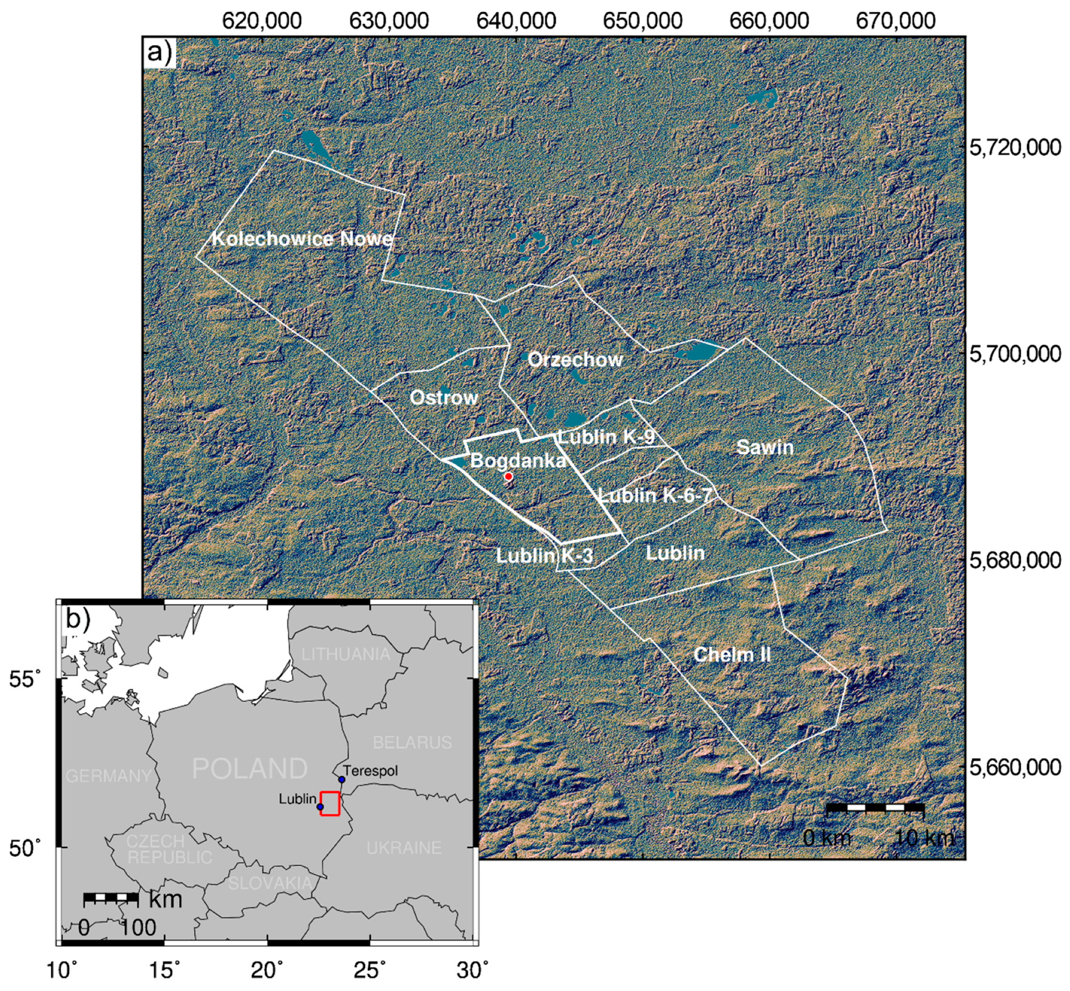
Figure 1. (a) The Lublin Coal Basin location over the 1′’ Digital Elevation Model (DEM) Shuttle Radar Topography Mission (SRTM) background. The black polygons represent the documented coal deposits, the thicker line covers the Bogdanka deposit and the Bogdanka Coal Mine is indicated by the red dot. Map representing Lublin Coal Basin is in WGS 84 /Universal Transverse Mercator (UTM) zone 32N projection. (b) Map showing localization of Lublin Coal Basin in Poland, in WGS84 projection.
Sustainability 12 09338 g001
Figure 2. Monthly average sum of precipitation calculated based on the meteorological data collected over the studied period [39].
Sustainability 12 09338 g002
Figure 3. Identification of floodplains in the Bogdanka hard coal mining region, based on Modified Normalized Difference Water Index (MNDWI) values difference between 2015 and 2019. The black solid polygon represents the Bogdanka deposit.
Sustainability 12 09338 g003
Figure 4. (a) Normalized Difference Vegetation Index (NDVI) index range; (b) floodplains identified based on spectral indices for the studied area. The black solid polygon represents the Bogdanka deposit.
Sustainability 12 09338 g004
Figure 5. Top: Maps of cumulative Line of Sight (LOS) displacements from October 2015; middle: cross-section AA’; bottom: cross-section BB’ of cumulative displacements over the studied period. The red border in the upper part of the map indicates the Brzezno Lake Reserve.
Sustainability 12 09338 g005
Figure 6. (a) Soil types; (b) groundwater levels used in the analysis, acquired from the geological and hydrogeological maps. The black solid polygon represents the Bogdanka deposit.
Sustainability 12 09338 g006
Figure 7. Block diagram of the performed analysis.
Sustainability 12 09338 g007
Figure 8. (a) terrain elevation (based on the SRTM 1” DEM); (b) terrain slope; (c) terrain aspect, calculated from the terrain elevation data. The black solid polygon represents the Bogdanka deposit.
Sustainability 12 09338 g008
Figure 9. Correlation matrix of explanatory features.
Sustainability 12 09338 g009
Figure 10. Histograms and statistics of continuous variables, classified into flooded and non-flooded areas.
Sustainability 12 09338 g010
Figure 11. Histograms of discrete variables, classified into flooded and non-flooded areas.
Sustainability 12 09338 g011
Figure 12. Result of the Random Forest machine learning algorithm, showing the classification of the areas as flooded and non-flooded, over the studied area.
Sustainability 12 09338 g012
Figure 13. Left: feature importance in the Random Forest prediction of flooded areas; Right: feature impact on the Random Forest prediction of flooded areas.
Sustainability 12 09338 g013
Figure 14. GWR model: map of residuals.
Sustainability 12 09338 g014
Figure 15. Geographically Weighted Regression (GWR) model: spatial variability of coefficients. Black solid rectangles represent significant areas, characterized in text.
Sustainability 12 09338 g015
Table 1. Selected studies on the use of active and passive remote sensing in monitoring the impact of exploitation on the environment.
SourceArea of InterestIssuesSatellite DataMethods
[21]Amynteon mine (Greece) Impact of mining activities on terrain and water resourceLandsat-5 and Landsat-7, SPOT and ASTERUnsupervised classification techniques in GIS
[22]The PT Freeport Indonesia (Indonesia)Impact of mining activities on land coverLandsat-5Three false-color composite image
[23]Lignite mine “Belchatów”, (Poland)Impact of mining on hydrogenic habitatsLandsat-5 and Landsat-7Normalized Difference Vegetation Index (NDVI)
[24]Coal mine in Tangshan, (China)Impact of mining activities on terrainETM, SPOT-4, SPOT-5 and IKONOSMulti-spectral composite imagery
[25]Lignite mines (eastern Germany)Monitoring of the environment and reclaimed areasLandsat-TM and ERS-1Maximum Likelihood Classification of Landsat Thematic Mapper
[27]Coal mine in Gangwon-do (South Korea)Subsidence analysis in a mining areaJERS-1SBAS algorithm and GIS
[28]Two coalfields, Bulianta and Shangwan (China)Determination of common features of deformations detected in two areasALOS PALSARSBAS processing
[29]Coal mines in the Greater Region of Luxembourg (the French–German border)Mapping coal mining-related ground subsidence and upliftERS-1/2 and ENVISATSBAS processing
[30]The Northumberland and Durham coalfield (United Kingdom)Investigation terrain motion and groundwater level change phenomenaERS, ENVISAT and Sentinel-1Intermittent SBAS technique
[31]The South Wales Coalfield (United Kingdom)Monitoring of uplift caused by pumping groundwaterERS-1/2Intermittent SBAS technique
[20]Mine of coal and metal ores, Kirchheller Heide (Germany)Landscape dynamics and extensive soil movementLandsat ETM+Random Forest, Spectral Mixture Analysis (SMA), Normalized Difference Vegetation Index (NDVI)
[32]The Three Gorges Reservoir area (China)Prediction of groundwater level-Classification and regression tree (CART)
[26]The southwestern part of Ritu county, BahrainAssessment of groundwater potentialLandsat 8 OLI 7/5/3Multi-criteria decision model (MCDM) integrated with decision tree techniques (C5.0) and CART
[33]Sichuan Province (China)Predicting displacement of landslide-Least Square Support Vector Machines (LSSVM), Genetic Algorithm (GA)
[34]Darling River Floodplain (Australia)Modeling of wetlands-Random Forest
Table 2. The main studies on the use of active and passive remote sensing in monitoring the impact of exploitation on the environment.
IndexMathematical Formula 1Source
NDVI N I R R E D N I R + R E D [43]
MNDWI G R E E N S W I R 1 G R E E N + S W I R 1 [44]
1 NIR, Red, Green and SWIR1 correspond to the reflectance value in the Near-IR, Red, Green and Mid-IR channels, respectively (1565–1655 nm).
Table 3. List of variables used in the analysis.
No.NameDescription
1NDVI RangeBased on the Sentinel-2 imagery obtained for April, during the years 2016–2019 (Section 2.3)
2LOS terrain displacementsBased on the Sentinel-1 SAR data, 5 rasters: October 2015, April 2016–2019 (Section 2.4)
3Groundwater depthDivided into 3 categories (Section 2.5)
4Geological classification of soilDivided into 3 categories, depending on the soil susceptibility to water retention (Section 2.5)
5DEMSRTM 1”
6SlopeBased on the DEM, values in %
7ExposureBased on the DEM, values generalized to 4 main geographic directions and flat terrain
8Identified floodplainsBased on the MNDWI values (Section 2.3)
Table 4. Random Forest model: accuracy metrics.
PrecisionRecallF-1 Score
Non-flooded area99.97%99.99%99.98%
Flooded area93.42%75.85%83.73%
Table 5. Random Forest model: confusion matrix.
Predicted
Non-Flooded AreaFlooded Area
TrueNon-flooded area3,173,140238
Flooded area10763380
Table 6. GWR model: coefficients statistics.
VariableMeanStd.Min.MedianMax.p-Value
Cumulative displacement−0.010.08−0.660.000.330.00
NDVI maximum difference−0.020.14−0.540.000.610.54
Terrain height−0.100.33−8.130.002.280.00
Slope0.000.14−1.980.004.060.00
Publisher’s Note: MDPI stays neutral with regard to jurisdictional claims in published maps and institutional affiliations.