Article

Analytical Method for Calculating Sustainable Airport Capacity

Department of Civil, Building and Environmental Engineering, Sapienza—University of Rome, Via Eudossiana 18, 00186 Rome, Italy
*
Author to whom correspondence should be addressed.
Sustainability 2020, 12(21), 9239; https://doi.org/10.3390/su12219239
Submission received: 22 September 2020 / Revised: 30 October 2020 / Accepted: 4 November 2020 / Published: 6 November 2020
(This article belongs to the Special Issue Toward Sustainability: Airport Risk Assessment)

Abstract

:
Capacity is the attitude of an airport to manage a number of operations in a given time interval within a fixed maximum delay (and under given safety conditions). Capacity studies are commonly carried out on five levels of analysis according to the required detail in order to identify the best option that balances economic, logistic and safety issues. This study focuses on level 3 (i.e., analytical methods) developing a calculation model to assess the runway capacity. The model was calibrated by comparing the outputs of different airport configurations with those provided by the circular of the Federal Aviation Administration Airport Capacity and Delay. The model was well calibrated with maximum differences in the analyzed configurations that stood at 1 or 2 movements/hour. The runway capacity of an international airport was calculated and compared to that of the entire airside, assessed through fast time simulation, in a previous study. The analytical model provides runway capacity slightly higher than that of the entire air system, as it cannot evaluate all the critical issues present in the airport that reduce its maximum theoretical capacity. Therefore, depending on the degree of detail required, you can use the developed model or the simulation software; the use of the latter is possible when the airside infrastructure does not adequately support the runway system or in cases of advanced design level.

1. Introduction

Air transport is continuously growing. According to IATA, 4.4 billion passengers were transported worldwide in 2018 with an increase of 6.9% compared to 2017 [1]. To meet this rapid growth, the infrastructure performance should be adequate: over the years, several definitions have been linked to the airport capacity—i.e., the ability of an airport to manage a certain number of operations (landings/take-offs) in a given time interval [2]. Moreover, an important trend for airline industry evolution should be considered: the rapid growth of the emerging global mega-carriers [3]. Therefore, the verification of the adequacy or otherwise of an infrastructure is necessary in order to evaluate:
  • Demand growth forecasts that should be met [4];
  • Adoption of new procedures to which the airport is forced to submit (for example, they may concern ground handling, approach or removal procedures);
  • Any delays in operations, caused by the current traffic demand, that influence the value of sustainable airport capacity (i.e., according to Airport Cooperative Research Program (ACRP) Report 104, “a measure of the hourly capacity that can realistically be achieved for several consecutive hours” [5]; it is generally 10–20% lower than saturation capacity);
  • Issues in terms of safety, environment and cost in order to minimize their burdens.
An airport is a complex system in which components of different nature interface, even those extremely different from each other [6]. Indeed, many factors affect the overall capacity of the infrastructure [7], including the configuration, number, spacing and orientation of the runway system, the configuration, number, size of taxiways, runway exits and apron areas, traffic routes, the size and mix of aircrafts using the facilities, the weather conditions and the existence and frequency of occurrence of wake vortices, the approach and departure procedures [8], the possible presence of nearby airports, the characteristics of the radar systems, possible adoption of anti-noise procedures and the workload to which the tower controllers are subjected [9,10]. Capacity analysis can take place by analyzing the influence of these elements on economic, logistic and safety issues [11]. Moreover, strategies adopted to increase airport capacity affects environmental sustainability: air transport accounts around 10% of all transport energy consumption in the EU and is responsible for approximately 15% of all CO2 emissions [12,13]. Therefore, any modification of airport capacity affects and depends on the environmental policy of airport operators and the social and transport organization [14,15].
Five levels of model refinement are currently used in the calculation of the capacity of an airport infrastructure [16] based on the type of application, the modelling hypotheses, the detail of the input parameters, the costs related to the analysis and the skills required by the user to effectively use the tools for each level of analysis. We can briefly distinguish [16]:
  • Level 1: Table lookup. The actual configuration is compared to a standard one. This level is suitable for runways only and simply airfields and only minimal information on runway configuration and aircraft fleet mix are required. Chapter 2 of FAA AC 150/5060-5 [2] provides an example of level 1 analysis.
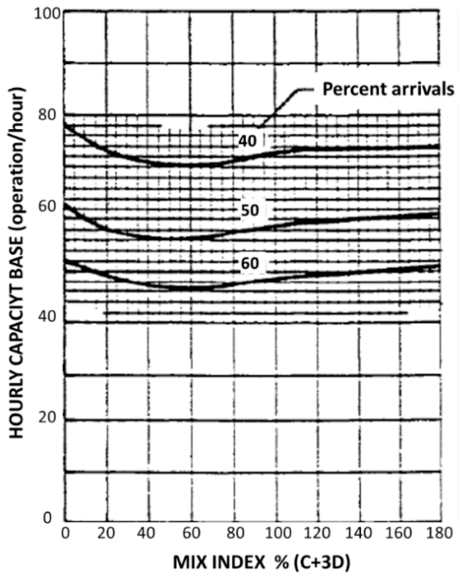
  • Level 2: Charts, monographs and spreadsheets. This level is suitable for runways only and simply airfields, but the input data require a better knowledge of the traffic in the airport and more information on the airport layout (taxiways and gates). Chapter 3 of FAA AC 150/5060-5 [2] presents an example of level 2 analysis.
  • Level 3: Analytical capacity models. Even if level 3 is suitable for runways only, it allows the analysis of moderate size airports and some more information in inputs on aircraft fleet mix, aircraft final approach speeds, aircraft separations, and air traffic control (ATC) rules.
  • Level 4: Airfield capacity simulation models. Capacity planning of complex airfields or regional airfield/airspace systems can be carried out and it requires more detailed input data than the previous levels. Arrival and departure flight track geometries and aircraft fleet mix by runway shall be known in addition to the complete airport configuration.
  • Level 5: Aircraft delay simulation models. These models, also called Fast Time Simulation (FTS), are the most advanced tools for the study of the whole airport. The capacity assessment of complex airfields or regional airfield/airspace systems can be performed and the greatest level of detail about aircraft flight schedule and airfield and airspace configurations, including taxiing routes and aircraft parking position area required [17,18,19].
Level 3 (i.e., analytical methods) uses a series of equations to calculate the minimum separation time between two planes and to go back to the value of the maximum capacity of a runway. Among them, the best-known software is the Airfield Capacity Model (ACM), created by the Federal Aviation Administration (FAA); other available tools are the FAA spreadsheet (developed during the “ACRP Project 03-17” and released free of charge) [17] and the LMI Runway Capacity software, which instead is proprietary [20]. As with levels 1 and 2, the level 3 analytical methods are no longer updated. In fact, the models do not reflect the recent changes in airport procedures, air traffic control procedures, information technology, available data, introduction of different performance aircrafts, and classification of aircraft in the wake turbulence categories (WTC). The wake turbulence phenomenon derives from the forces involved necessary for the aircraft to sustain itself in flight and is the one that most influences the sustainable airport capacity. The high-pressure air present on the lower area of a wing tends to move, through the wing tip, to the upper area [21]; this causes the release of two counter-rotating vortices and therefore the formation of a turbulence zone behind the plane. Recent studies [19] have shown that in addition to the weight of the aircraft, the turbulence of wake is related to the speed of the aircraft and its wingspan. The new reclassification, which goes by the name of WTCReCat (Wake Turbulence Re-categorization) [22,23], provides for a subdivision into six turbulence classes that are used to define the minimum horizontal separation to be adopted in order to guarantee operational safety. Now, there are no updated, user friendly and useful free tools for estimating the runway capacity of an airport. So very often it necessary to resort to simulation analyses, which is extremely expensive, in order to obtain reliable data, as confirmed by recent studies [24]. For these reasons, in this study a new spreadsheet has been created in Microsoft Excel®. It allows for calculating, under suitable assumptions, the runway capacity in single or multiple parallel systems. This simple method could be used in a preliminary planning phase. Today, computer technology allows for using much more sophisticated methods, such as the fast time simulation; however, they are quite expensive and above all require the use of highly specialized personnel. This, therefore, involves very high costs that could be faced only to verify choices that have been preliminarily studied. The purpose of this article is therefore to demonstrate how much an analytical method can be entrusted to it in the screening of all possible solutions for planning airport operations.

2. Methods

The runway capacity value is calculated as the inverse of the separation time E (h), between two aircrafts. The analytical model for the assessment of the runway capacity presented in this article has been developed under the following assumptions:
  • Probabilistic sequencing of operations (arrival/departure): the actual traffic mix monitored in the airport is analyzed according to the six WTC to obtain the Pij matrix that describes the probabilities of presence of a class “i” aircraft (leader aircraft) followed by a “j” class aircraft (follower aircraft);
  • Continuous demand of arrivals: local problems or interference which can reduce landing operations are neglected;
  • Continuous demand of departures: in this case, local problems or interferences that can reduce take-off operations are also neglected;
  • Analytical evaluation of the runway occupancy time (ROT) for each WTC;
  • Constant aircraft speed along the terminal approach path equal to the certified approach speed (Vapp) for each WTC;
  • Ideal weather conditions.
The calculation of the departing single runway capacity is performed by the temporal separation matrix Cij, deriving by the sum of the minimum WTC separation δ and the additional time buffer.
The sum of the matrix products between Cij and Pij will make it possible to obtain the average departure time E (h) for the specific airport, from which the departure capacity value is calculated. To calculate the incoming capacity, the separation time Tij between two generic planes is estimated first based on the minimum distances required by the WTC. In the closing case [20], defined as the case where the leading plane i has a lower speed than the follower plane j, the separation time Tij at the threshold is (Equation (1)):
T i j = δ V j
where
  • δ = minimum separation distance specified by air traffic rules;
  • γ = length of the terminal approach path;
  • vj = speed of the follower plane.
Instead, in the opening case [20], this is defined as the case in which the leading plane i has a higher speed than the follower plane j (Equation (2)):
T i j = δ V j + γ V j γ V i
where Vi is the speed of the leading plane.
The buffer time Bij [25] is added to the minimum separation time Tij to take into account the positional errors caused by the ATC systems and by the pilots.
In the closing case (Equation (3)):
B i j = σ 0 q v
whereas in the opening case (Equation (4)):
B i j = σ 0 q v δ i j 1 V j 1 V i
setting Bij = 0 if negative.
Finally, considering the probability matrix Pij of aircraft presentation in the airport, the average departure time E (h) is given by Equation (5):
B i j = σ 0 q v δ i j 1 V j 1 V i
After landing, the time required for each aircraft to exit the runway (Dij) depends on the runway occupancy time (ROT), considering a buffer time to include the errors due to the violation of separation distance and radar system. Dij is evaluated by means of the matrix elements Dij4 (Equation (6)):
D i j = R O T i + q v σ 0 2 + σ R O T 2
where qv is the value in correspondence of which the function of the normal cumulative distribution is (1 − Pv) [26]; Pv is the probability of violation of the minimum distance (%); σ0 is the positional error of radar control systems (sec); σROT is the standard deviation of ROT.
The separation distances adopted by the ATC must be compatible with the time required for each aircraft to exit the runway. If the outcome of the check is positive, the elements of the matrix (Tij + Bij) must be greater than the respective elements of the matrix Dij.
The model also computes the capacity of a runway used in mixed mode, that is, by inserting departures between two successive arrivals. First, the Gij matrix of the minimum gaps required for sequencing a departure between two consecutive arrivals (Figure 1) derives from Equation (7):
G i j = R O T i + D i j V j .
The required gaps Gij are compared with the generic arrival separation times (Tij + Bij) in order to identify the matrix Mij, representative of the number of departures that can be inserted between two arrivals. Finally, the number of departures in mixed capacity while maintaining 100% of the arrivals is calculated by adding the matrix products between the Mij and Pij and multiplying the result by the number of hourly arrivals foreseen by the model.
If the runway is used in mixed mode with different arrivals/departures ratios, the parameter of additional arrival separation α can be used in the model.
Because α increases the minimum WTC distances, the arrival capacity of the runway is reduced while the departure capacity is increased as the times available for inserting a take-off between two arrivals increase.
At airports with parallel runway systems, the sequence of the operations depends on the distance between the runways [24]:
  • Take-offs can be independent if the runway distance is greater 760 m and the routes divergences is greater than 15° (Figure 2);
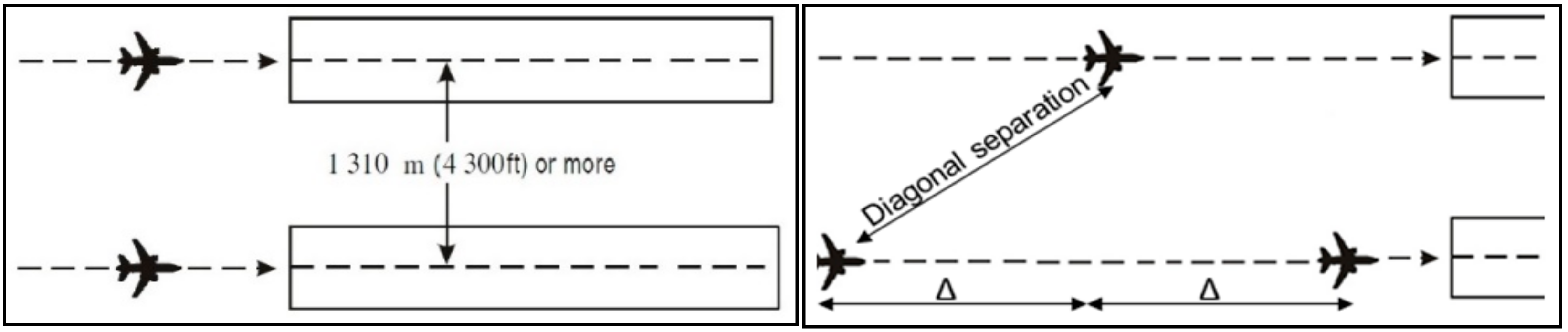
  • Landing can be independent if the runway distance is greater 1310 m, otherwise a “chessboard” configuration has to be considered. With this aim, the model takes this into account a minimum diagonal spacing d2. This allows for having a distance between two approaching aircraft on the same runway compatible with the movement of other planes landing on the adjacent runway (Figure 3).

3. Case Study

The model has been applied to study the capacity of a high traffic airport with a standard layout: two parallel 3860 m runways (grey lines in Figure 4), whose distances between their centerlines are 840 m. The airport is classified 4F, according to [26]. Both runways are equipped with ILS and the operations are performed according to Instrumental Flight Rules (IFR).
Segregated operations on the two parallel runways are normally performed on the two parallel runways (Figure 5a), except during traffic peaks, when each runway is used in mixed mode (Figure 5b).
The third parallel runway is planned in the medium-term master plan. The new runway (grey line in Figure 6) is shorter, parallel, staggered at 1200 m from the previous ones.
This layout allows for greater flexibility in the runways use; indeed, the distance between the existing runways and the new runway is sufficient to allow for independent contemporary landings. The use of the runway system provides for mixed mode the use of the new runway (no. 3 in Figure 7), only arrivals from runway no. 1 in Figure 7 and only departures on runway no. 2 in Figure 7.
In 2018, more than 180,000 movements were registered in the examined airport (Figure 8 presents monthly details of aircrafts movements).
The capacity analysis considered the traffic of the average day of the busiest month, which comprised a total of 563 daily movements on average. This is the value of the occurred daily movements nearest to the statistical average value: in the examined airport, this was 564 movements, which happened on 18 August (Figure 9).
Figure 10 shows the percentage share of the airplanes in the traffic fleet in the airport and Table 1 lists the WTC ReCAT of each aircraft. Traffic analysis of the average peak day of the busiest month has resulted in the percentage composition of the turbulent wake classes shown in Figure 11.
The runways capacity has been performed with three calculation levels, with regard to the following scenarios:
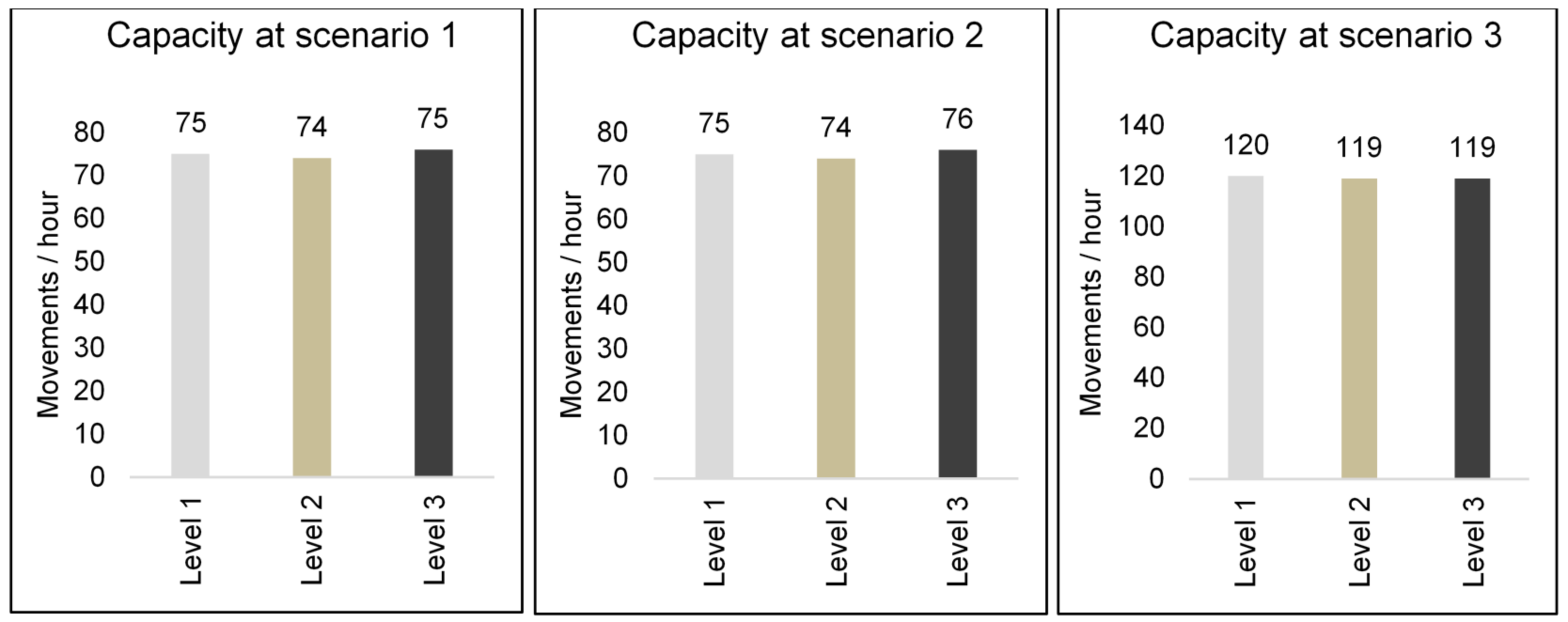
  • Scenario 1: two-runway configuration with segregated use;
  • Scenario 2: two-runway configuration with mixed mode use;
  • Scenario 3: three-runway configuration with mixed mode use of one runway and segregated of the other two.
At level 1, the analysis was carried out by means of the method proposed by [2]: this is based on the comparison of the studied airport with the 19 standard configurations and takes into account the aircraft classes listed in Table 2.
The method defines a “Mix index” for each configuration, as defined in Equation (8), to be used as a parameter to the look-up tables:
Mix Index = (C + 3D) %
where C is the percentage of Class C aircraft and D is the percentage of Class D aircraft (Table 2).
Given traffic data are listed in Table 1. The values of C and D are taken from Figure 11. In this case, the mix index = (67.7 + 13.3) + 3 × (1.1 + 9.4 + 5.3) = 128.4. Table 3 lists the input data considered in the capacity assessment at level 1.
The results are summarized in Table 4: the capacity values are 75 movements/hour in scenarios 1 and 2 and 120 movements/hour in scenario 3.
The level 2 analysis was carried out, referring to Federal Aviation Administration [2]. The problem is solved using diagrams provided by the FAA circular for a large number of runway uses and configurations. For the case study, the diagram in Figure 12 is available for scenario 1.
At this level, it is possible to consider the number of “Touch and Go” operations and the characteristics of the airside, such as the number and location of the runway exit taxiways, considering two the multiplier coefficients.
In the examined airport, there are 2 exit taxiways, located at 1810 m and 2120 m from the thresholds and according to FAA guideline, the multiplier Exit Factor (E) is equal to 1. Because in this airport there are no “Touch and Go” operations, the factor T is equal 1. Finally, considering the arrivals in IFR conditions with a percentage equal to 40% in the peak hour, the assessed capacity is equal to 74 movements/hour. With the same procedure and the suitable diagram, the capacity assessment is 74 movements/hour in scenario 2 and 119 movement/hour in scenario 3. At level 3, the capacity assessment which been carried out by the analytical model herein presented.
For the 6 aircraft classes, WTC ReCAT, the values of ROT and Vapp were defined as weighted average on the number of movements of each aircraft included in the class. The results are listed in Table 5.
Table 6 summarizes the other parameters considered in the analytical model.
The input values adopted are those suggested in [21] and [24] and are representative of the conditions existing at the time when calculation levels 1 and 2 were devised. In this way, the accuracy of the analytical model was verified. With the data in Table 6, the capacity value obtained is 75 movements/hour in scenario 1, 76 movements/hour in scenario 2 and 119 movements/hour in scenario 3, similar to those obtained with the calculation levels 1 and 2, as shown in Figure 13.
Once the model was calibrated, the input values of the positional error of radar control systems and the diagonal separation were updated to better represent the current operating conditions.
Due to modern radar response characteristics, the parameter σ0 can be considered equal to 8 sec. The diagonal separations, on the other hand, were defined based on the procedures implemented in Italy by the flight controllers and a d2 value of 2 NM was adopted.
In scenarios 2 and 3, the capacity was recalculated considering the optimization between the arrivals/departures on the runways to obtain the maximum capacity value for each configuration (balanced conditions). These values are equal to 88 movements/hour in scenario 2 and at 124 movements/hour in scenario 3. Scenario 1 was omitted since the use of the segregated condition does not allow for the calculation of the system balanced capacity.

4. Result and Discussion

A sensitivity analysis was performed on the analytical model to evaluate its response to the input parameters, varied within the intervals described in Table 6. The results are shown in Figure 14, expressed with a tornado diagram; in this graph, the amplitude of the loop with respect to the axis of the tornado represents the sensitivity of the model to the variation of each parameter. The turns take on a lighter color if the variability of the output is related to a more uncertain input parameter or darker color if the change in the output is linked to a more stable input.
Figure 14 shows that the sensitivity of the output is mainly related to the variation of the parameters that describe the ATC error and the departure/arrival separation d1; however, these variables assume certain values within their interval of definition, as the former depends on the radar instrumentation reliability while the second is defined by the relevant authorities. Instead, the model is not sensitive to other parameters that are not easily evaluable, such as pilot mistakes, length of the terminal approach path, additional buffer on departure, ROT standard deviation. So, it is possible to conclude that the overall sensitivity of the model is rather moderate.
The results obtained with the level 3 model were compared with the sustainable and saturation capacity values obtained at calculation level 5 by means of FTS, carried out in a previous study [24]. This study estimated the balanced capacity of the airport equal to 72 movements per hour in scenario 2, and 114 movements per hour in scenario 3. In this case, the capacity values refer to the entire air system of the infrastructure and are not limited exclusively to the runway capacity. Figure 15 summarizes the results obtained in the above described scenarios.
The graphs show that the runway capacity given by level 3 model is 18.2% greater in scenario 2 and 8.1% in scenario 3 than the capacity of the entire airside resulting from FTS (level 5). The difference arises because the calculation model, even if properly calibrated, provides the ideal answer representative of the maximum potential of the infrastructure, under the assumptions of continuous arrival and departure demand and minimum separations adopted by the air traffic controllers. Actually, within the airside of the airport, there may be bottlenecks that limit the overall capacity of the system: they are generally due to inadequate exit connections, deficiencies in the system of traffic routes, interference in parking lots, difficulty in maneuvering in aprons, etc.
Furthermore, the three-level model does not capture any aspects that may be present in a specific airport and that may limit its capacity; for example, in the case study, due to the location of the terminal in the south area, the airplanes that have to operate in the north runway need to cross the runway in the south area. The use of simulation software instead allows for a more extensive and in-depth analysis of the systems on the airside, especially for an airside that does not adequately support the runway system. In this case, the analytical models overestimate the capacity.
However, the obtained values in terms of movements/hour impact on services offered to passengers and on surrounding environment—stakeholders cannot overlook the relationship between airport capacity and sustainability, with regard to different and often conflicting interests (e.g., noise, number of transported passengers, energy saving, air quality management, public health, landscape enhancement). Therefore, several parameters should be considered with a multi-criteria analysis [27].

5. Conclusions

The assessment of the capacity is the main tool to evaluate the airport capacity. This evaluation can be carried out with a different degree of depth, according to the detail required, commonly by five levels of analysis. At level 3 of this classification of airport capacity estimation methods, there are currently no updated models—that provided by the FAA is a closed software and the parameters related to the new technologies adopted in most commercial civil airports are not updated. On the one hand, in fact, there are methods (levels 1 and 2) that are too simplistic and no longer updated, such as those proposed by the FAA AC circular: 150/5060-5, which attempt to describe real situations by approximating them to predefined configurations. On the other hand, the most recent simulation techniques (levels 4 and 5) allow for extremely detailed but very expensive analysis; therefore, if high calculation precision is not required, such as for preliminary or planning studies, simulation may not be the best choice. For these reasons, an analytical model, based on a spreadsheet, was implemented on Microsoft Excel® for assessing the runway capacity of an airport, needed because the only available alternative is proprietary software. The model was calibrated on the results obtained at levels 1 and 2, using input data representative of the typical conditions existing when these methodologies were defined. The model results were well calibrated—indeed the maximum differences with respect to the various configurations analyzed are equal to one or two movements per hour. Finally, using the most suitable parameters to represent the current conditions, the runway capacity of an airport case study was estimated and compared with the sustainable and saturation capacity of the entire airside system calculated through FTS in a previous study. The results show that, for this case study, the runway capacity is approximately 18% greater than the airside capacity in scenario 2 and 8% in scenario 3. The difference arises because the implemented model provides, under certain hypotheses, a value equal to the maximum potential of the infrastructure, not considering the particular critical issues affecting an airport that can reduce its movement.
We can conclude that the developed spreadsheet or simulation software can be used depending on the degree of complexity of the system, the in-depth analysis required and the resources available. The use of the simulation can therefore be limited to cases where the configuration of the infrastructure on the airside does not adequately support the runway system or in cases of advanced design level.

Author Contributions

Conceptualization, P.D.M., L.M. and G.R.; methodology, G.R.; software, G.R.; validation, L.M. and G.R.; formal analysis, P.D.M., L.M. and G.R.; investigation, G.R.; data curation, P.D.M. and G.R.; writing—original draft preparation, P.D.M.; review and editing, P.D.M., G.R. and L.M.; supervision, P.D.M. All authors have read and agreed to the published version of the manuscript.

Funding

This research received no external funding.

Conflicts of Interest

The authors declare no conflict of interest.

References

  1. IATA. Word Air Transport Statistics. Available online: https://www.iata.org/en/publications/store/world-air-transport-statistics/ (accessed on 10 February 2020).
  2. Federal Aviation Administration. Airport Capacity and Delay; AC: 150/5060-5; U.S. Department of Transportation, Federal Aviation Administration: Washington, DC, USA, 1983. Available online: https://www.faa.gov/documentLibrary/media/Advisory_Circular/150_5060_5.pdf (accessed on 5 November 2020).
  3. De Neufville, R.; Odoni, A.R. Airport Systems: Planning, Design and Management, 2nd ed.; MacGraw Hill: New York, NY, USA, 2003; ISBN 978-0-07-177058-3. [Google Scholar]
  4. Tascón, D.C.; Díaz Olariaga, O. Air traffic forecast and its impact on runway capacity. A System Dynamics approach. J. Air Transp. Manag. 2021, 90, 101946. [Google Scholar]
  5. ACRP. Defining and Measuring Aircraft Delay and Airport Capacity Thresholds; Report 104; Transportation Research Board: Washington, DC, USA, 2014. [Google Scholar]
  6. Ashford, N.J.; Coutu, P.; Beasley, J.R. Airport Operations, 3rd ed.; McGraw-Hill Education: New York, NY, USA, 2012. [Google Scholar]
  7. Horonjeff, R.; McKelvey, F.; Sproule, W.J.; Young, S.B. Planning & Design of Airports, 5th ed.; Mc Graw Hill: New York, NY, USA, 2010. [Google Scholar]
  8. Di Mascio, P.; Cervelli, D.; Comoda Correra, A.; Frasacco, L.; Luciano, E.; Moretti, L. Effects of Departure MANager (DMAN) and Arrival MANager (AMAN) systems on airport capacity. J. Airpt. Manag. 2021. accepted paper. [Google Scholar]
  9. Di Mascio, P.; Carrara, R.; Frasacco, L.; Luciano, E.; Moretti, L.; Ponziani, A. Influence of Tower Air Traffic Controller workload and airport layout on airport capacity. J. Airpt. Manag. 2021. accepted paper. [Google Scholar]
  10. Eurocontrol. Airport Capacity Assessment Methodology; ACAM Manual; v.1.1; Eurocontrol: Brussels, Belgium, 2016; Available online: https://www.eurocontrol.int/sites/default/files/publication/files/nom-apt-acap-acamman-v1-1.pdf (accessed on 5 November 2020).
  11. Graham, B.; Guyer, C. Environmental sustainability, airport capacity and European air transport liberalization: Irreconcilable goals? J. Transp. Geogr. 1999, 7, 165–180. [Google Scholar]
  12. Stanners, D.; Bourdeau, P. (Eds.) Europe’s Environment: The Dobris Assessment; Office for Official Publications of the European Communities: Luxembourg; European Environment Agency: Copenhagen, Denmark, 1995. [Google Scholar]
  13. Ivković, I.; Čokorilo, O.; Kaplanović, S. The estimation of GHG emission costs in road and air transport sector: Case study of Serbia. Transport 2018, 33, 260–267. [Google Scholar]
  14. Button, K.; Nijkamp, P. Social change and sustainable transport. J. Transp. Geogr. 1997, 5, 215–218. [Google Scholar]
  15. Čokorilo, O.; Dell’Acqua, G. Aviation Hazards Identification Using Safety Management System (SMS) Techniques. In Proceedings of the 16th International Conference on Transport Science ICTS 2013, Portorož, Slovenia, 27 May 2013; pp. 66–73. [Google Scholar]
  16. Čokorilo, O. Human Factor Modelling for Fast-Time Simulations in Aviation. Aircr. Eng. Aerosp. Technol. 2013, 85, 389–405. [Google Scholar]
  17. Bubalo, B.; Daduna, J.R. Airport capacity and demand calculations by simulation—The case of Berlin-Brandenburg International Airport. NOTNOMICS Econ. Res. Electron. Netw. 2011, 12, 161–181. [Google Scholar]
  18. Ignaccolo, M. A simulation model for aiport capacity and delay analysis. Transp. Plan. Technol. 2003, 26, 135–170. [Google Scholar]
  19. ACRP. Evaluating Airfield Capacity. Transportation Research Board; Report 079; Transportation Research Board: Washington, DC, USA, 2012. [Google Scholar]
  20. FAA. Pilot and ATC Guide to Wake Turbolence. 2016. Available online: https://www.faa.gov/training_testing/training/media/wake/04sec2.pd (accessed on 17 February 2020).
  21. Eurocontrol. European Wake Turbulence Categorisation and Separation Minima on Approach and Departure, 1st ed.; Eurocontrol: Brussels, Belgium, 2015; Available online: https://www.eurocontrol.int/publication/european-wake-turbulence-categorisation-and-separation-minima-approach-and-departure (accessed on 5 November 2020).
  22. NASA. Estimating the Effects of the Terminal Area Productivity Program; s.n. 201682; NASA Langley Technical Report Server: Hampton, VA, USA, 1997.
  23. Cavusoglu, S.S.; Macario, R. Minimum delay or maximum efficiency? Rising productivity of available capacity at airports: Review of current practice and future needs. J. Airpt. Manag. 2021, 90, 101947. [Google Scholar]
  24. Di Mascio, P.; Cervelli, D.; Comoda Correra, A.; Frasacco, L.; Luciano, E.; Moretti, L.; Nichele, S. A critical comparison of airport capacity studies. J. Airpt. Manag. 2020, 14, 307–321. [Google Scholar]
  25. Federal Aviation Administration. Parameters of Future ATC Systems Relating to Airport Capacity/Delay; EM-78-8A; U.S. Department of Transportation, Federal Aviation Administration: Washington, DC, USA, 1978. Available online: http://www.tc.faa.gov/its/worldpac/techrpt/em78-8a.pdf (accessed on 5 November 2020).
  26. International Civil Aviation Organization. Manual on Simultaneous Operations on Parallel or Near-Parallel Instrument Runways (SOIR); Doc 9643 AN/941; International Civil Aviation Organization (ICAO): Montreal, QC, Canada, 2004. [Google Scholar]
  27. Moretti, L.; Di Mascio, P.; Bellagamba, S. Environmental, Human Health and Socio-Economic Effects of Cement Powders: The Multicriteria Analysis as Decisional Methodology. Int. J. Environ. Res. Public Health 2017, 14, 645. [Google Scholar] [CrossRef] [Green Version]
Figure 1. Minimum gaps required for sequencing a departure between two consecutive arrivals.
Sustainability 12 09239 g001
Figure 2. Take-off independence requirements related to the distance between the runways and the divergence of the routes.
Sustainability 12 09239 g002
Figure 3. Landing independence requirements related to the distance between the runways.
Sustainability 12 09239 g003
Figure 4. Layout of the airport.
Sustainability 12 09239 g004
Figure 5. Operative modes of the two-runway system. Segregated Mode (a) and Mixed Mode (b).
Sustainability 12 09239 g005
Figure 6. Future layout.
Sustainability 12 09239 g006
Figure 7. Operative modes of the three-runway system.
Sustainability 12 09239 g007
Figure 8. Airport Monthly Movement.
Sustainability 12 09239 g008
Figure 9. Daily movements in the busiest month.
Sustainability 12 09239 g009
Figure 10. Percentage share of the airplanes in the traffic fleet.
Sustainability 12 09239 g010
Figure 11. Percentage share of WTC ReCAT in the traffic fleet.
Sustainability 12 09239 g011
Figure 12. Diagram provided by FAA AC 150/5060-5 at level 2 of capacity calculation for the configuration of the case study, page 43 in [2].
Sustainability 12 09239 g012
Figure 13. Runway capacity in scenarios 1-2-3 at levels 1-2-3.
Sustainability 12 09239 g013
Figure 14. Sensitivity analysis of the analytical model.
Sustainability 12 09239 g014
Figure 15. Runway capacity in scenarios 2-3 at level 3-5.
Sustainability 12 09239 g015
Table 1. Aircraft belonging to WTC ReCAT.
WTC ReCATAircraft
Super HeavyAirbus A380-800
Upper HeavyAirbus A330-200, Airbus A330-300, Airbus A350-900, Boeing B747-400
Boeing B747-800, Boeing B777-200, Boeing B777-300, Boeing B787-800, Boeing B787-900
Lower HeavyAirbus A300-600, Airbus A310, Boeing B757-200, Boeing B767-200, Boeing B767-300, Boeing B767-400
Upper MediumAirbus A320-Neo, Airbus A318, Airbus A319, Airbus A320, Airbus A321, Boeing B737-700, Boeing B737-800, Boeing B737-900, McDonnel Douglas MD82
Lower MediumATR42-300, ATR72-500, Boeing B737-300, Boeing B737-400, Bombardier A220, Bombardier CRJ-700, Bombardier DCH-8, Embraer EMB145, Embraer EMB170, Embraer EMB190, Fokker-100
LightBeechcraft 1900, Cessna Mustang, Cessna Excel, Dassault Falcon-2000, Embraer EMB120, Embraer Phenom 300, Gulfstream G150, Raytheon Hawker 800
Table 2. Aircraft Classification.
Aircraft ClassMaximum
Take-Off Weight
Engines NumberWake Turbulence Classification
A<5.7SingleSmall (S)
BMulti
C5.7–136MultiLarge (L)
D>136MultiHeavy (H)
Table 3. Input at level 1.
Input Level 1
Mix Index129%
Runway separation 1808m
Runway separation 21205m
Table 4. Capacity values at level 1 [2].
ScenarioRunway Configuration from FAA AC 150/5060-5Hourly Capacity (IFR)
1 and 2 Sustainability 12 09239 i001 Sustainability 12 09239 i00275 mov/hour
3 Sustainability 12 09239 i003 Sustainability 12 09239 i004120 mov/hour
Table 5. Weighted average of ROT and Vapp for the aircraft classes WTC ReCAT.
ParameterWTC ReCAT
LightLower MediumUpper MediumLower HeavyUpper HeavySuper Heavy
ROT [s]555552535048
Mix Fleet [%]3.213.367.75.39.41.1
Approach speed [kts]113128134139140141
Table 6. Parameters considered in the analytical model at calculation level 3.
DescriptionParameterRange (9), (10)Adopted Value
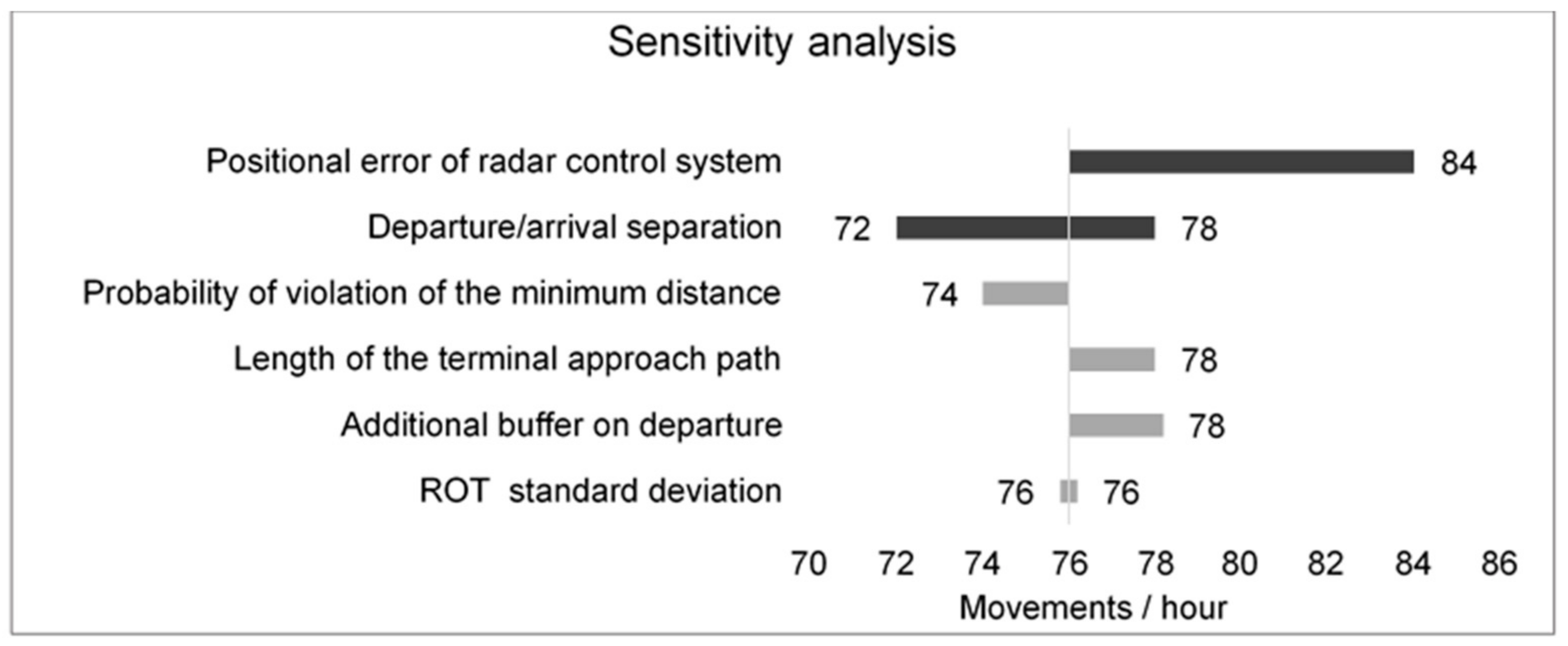
Positional error of radar control systemsσ0 [s]18 [s]–8 [s]18 [s]
Probability of violation of the minimum distancePv [%]5 [%]–1 [%]5 [%]
Value in correspondence of which the function of the normal cumulative distribution is (1-Pv)qv1.65–2.331.65
Length of the terminal approach pathγ [NM]5 [NM]–10 [NM]7 [NM]
Additional Buffer on departuret [s]5 [s]–30 [s]15 [s]
Departure/arrival separationd1 [NM]3 [NM]–5 [NM]4 [NM]
Diagonal separationd2 [NM]3 [NM]–2 [NM]3 [NM]
ROT standard deviationσROT [s]8 [s]–4 [s]8 [s]
Publisher’s Note: MDPI stays neutral with regard to jurisdictional claims in published maps and institutional affiliations.

