Abstract
This study integrated a focus on geographical, physical, and commercial characteristics to explore the commercial gentrification phenomenon and its related statistical summaries in the area of Garosu-gil in Seoul’s Sinsa-dong ward. In particular, this study first collected parcel and building data and corresponding attribute information and mapped the resulting datasets in a geographic information system (GIS) environment. We then examined gentrification issues per building and conducted statistical analyses to investigate spatial patterns of commercial gentrification, which were used to develop criteria for determining degrees of gentrification. Third, this study conducted correlation and regression analyses to quantify the strength of the linear relationship between pairs of variables associated with primary factors contributing to commercial gentrification, and used a geographically weighted regression model (GWR) to help understand and predict spatial relationships between significant variables. The results showed positive correlations between several variables and commercial gentrification in the study area, namely neighborhood-convenience facilities, building ages, store rents, new franchise and restaurant businesses, distance to subways, and the presence of multiple roads. Based on its finding, there are key contributions of this study as follows. The first significant contribution of this study is developing measurement of gentrification levels that can be used by policy makers at each of four stages of the gentrification process. Furthermore, this paper develops a comprehensive approach for spatially identifying gentrifying neighborhoods across multiple time periods in 2- and 3-dimensions. It eventually helps urban planners implement preventative or supportive programs to protect lower-income residents and small businesses and thereby engender more sustainable community development.
1. Introduction
1.1. Background
The term ‘gentrification’ was first coined by urban sociologist Ruth Glass in 1964 to refer to changes in social structure and housing markets observed in London’s inner city as lower-income residents were pushed out during the formation of upper-class neighborhoods []. Gentrification is generally defined as the displacement or replacement of lower-income households by those of upper-income households [,,]. As affluent people (i.e., higher-income newcomers) move to community areas for business and residency purposes, lower- and middle-income groups can no longer afford to live there, thus leading to population migration. Gentrification is an inevitable social phenomenon because people who run businesses naturally seek to increase their profits [,,]. The gentrification process in Seoul has resulted in significant commercialization in the area of Garosu-gil in the city’s Sinsa-dong ward [,,], an area now referred to as ‘Europe in Seoul’ known for its upscale boutiques, bars, galleries, restaurants, cafes, and shops []. Artist-residents who initially joined a community area provide new middle classes, but gentrification appears in multiple places in the area of interest. As commonly occurs, the gentrification process in Sinsa-dong began with influxes of culture artists and small businesspersons, who were attracted to the area due to low rents []. However, as the district has become more popular and received more attention in the broadcast media and on social networking sites, its shops have attracted increasingly large numbers of tourists and customers, and its floating population has grown dramatically. As large companies have invested greater capital into the area, the business district has greatly expanded, and rental and goods values have significantly increased to levels beyond the reach of existing residents, culture artists, and small businesspersons. Accordingly, this process has pushed the native residents out of the community area, and its traditional regional characteristics have rapidly diminished.
Although a number of gentrification studies have been conducted over the years, it is often challenging to collect reliable datasets, particularly visualized datasets, which can be used by policymakers to implement preventative or supportive programs. Furthermore, it is difficult to analyze gentrification processes or issues at fine spatial scales, such as parcels or building units, because doing so requires a great deal of time and cost. In addition, even when gentrification issues are understood by urban policymakers, it is less easy to standardize their degrees of importance. However, standardized and quantified criteria are needed to assist gentrified community areas in providing proper services and supports so as to engender a more sustainable process. To address these issues, this research analyzed spatial patterns of commercial gentrification in Garosu-gil. Specifically, the study integrated a focus on geographical, physical, and commercial characteristics to explore the commercial gentrification phenomenon and its related statistical summaries.
1.2. Related Studies
Although gentrification is generally a spatial and social practice that transforms a working-class area into one of middle-class residential or commercial use [], this process has taken on a variety of definitions over the last five decades []. More recently, commercial gentrification, which refers to displacements in the commercial environment of gentrifying community areas, has become a prevalent issue in major cities worldwide. As described by Zukin, the local cultural economy initiates regeneration strategies in commercialized urban spaces, which stimulates consumer spending and brings increased wealth and associated positive benefits to these areas as vibrant communities, shopping zones, and other attractions expand and generate large floating populations, such as tourists [,,,]. However, the regeneration of these commercialized urban spaces also results in increased property values, the displacement of people and capital, and an accelerated gentrification process, which are considered as negative outcomes []. Thus, although commercial gentrification is driven by local communities, the resulting displacement of neighborhood businesses leads to drastic physical, social, and economic changes [,], which at first have positive results in terms of the increase of floating populations and new demands []; however, as the process continues, the increased commercial amenities lead to increased property values and higher prices for goods and services as the neighborhood adapts to an influx of higher-income residents and larger companies [,,].
Numerous studies applying various research approaches have been conducted at various locations and spatial scales to understand gentrification issues. In the late 1970s, most research was focused on quantifying the magnitude of gentrification in order to determine the significance of the phenomenon []. For example, a major study focused on ‘market generated displacement’ associated with the rapid revitalization of San Francisco’s Hayes Valley neighborhood []. Later studies used traditional statistics from survey data to estimate displacement rates associated with urban revitalization and thereby achieve a more in-depth understanding of the negative impacts of gentrification [,,,,,]. In recent years, researchers have used geographic information system (GIS) environment and computational models to simulate aspects of neighborhood change accruing from gentrification []. For example, Parker and Pascual created a ‘living neighborhood map’ using GIS as a means to visualize how San Francisco’s working-class districts transformed into middle-class neighborhoods [], and Chapple used a similar approach to visualize changes in residential demographics in the Lake Merritt Neighborhood, Oakland, CA []. Chipman used an interactive mapping tool to visualize descriptive statistics related to injury and sociodemographic risk factors to inform public health policymaking []. Greene also introduced GIS applications for gentrification research []. In Seoul, Kwon used GIS mapping to visualize the distribution pattern of gentrification in Gyeongui Line Forest Park []. Maantay and Hong used census block group proximity and hot spot analyses to identify environmental gentrification based on proximity to community gardens in Brooklyn, New York [,].
A number of studies have used agent-based computational models, which integrate land use in GIS environment and other factors associated with gentrification to simulate residential segregation patterns in gentrifying areas [,,,]. For example, Jackson, Forest, and Sengupta used this approach to analyze rent change and associated residential dynamics in Boston, whereas Torrens and Nara developed an agent-based cellular model to examine property value changes and household relocation patterns during the early stages of the gentrification process in Salt Lake City, Utah. More recently, Eckerd, Kim, and Campbell developed an agent-based modeling technique to simulate policy choices, residential patterns, and displacement related to gentrification based on real estate market data from a range of US regions []. Similarly, Liu and O’Sullivan applied rent gap, filtering, and household life cycle theories to simulate the spatial dynamics of gentrification patterns [].
Among the wide range of gentrification studies, most have been conducted at the neighborhood or city scale, and relatively limited research has explicitly focused on this phenomenon at finer spatial scales, such as neighborhood parcels or building units. Moreover, even a number of gentrification studies have been conducted over the years, it is challenging to collect reliable datasets, particularly visualized datasets, which can be used by policymakers to implement preventative or supportive programs. Accordingly, it is difficult to analyze gentrification processes or issues at fine spatial scales, such as parcels or building units, because doing so requires a great deal of time and cost.
To address this gap, this research used GIS environment to visualize multiple variables associated with gentrification in three main categories: (1) ‘building types and uses’, (2) ‘transportation and roads’, and (3) ‘shopping centers’. Each category incorporated three to four variables, and a total of 11 variables were used to analyze neighborhood change dynamics in the study area. In addition, the study used a street view to investigate changes in store use. In particular, we first collected parcel and building data with attribute information and mapped the resulting datasets in a GIS environment. Second, we examined gentrification issues per building and conducted statistical analyses to investigate spatial patterns of commercial gentrification, which were used to develop criteria for determining degrees of commercial gentrification and eventually create a standard that assists gentrified areas and their residents. Third, this study conducted correlation and regression analyses to quantify the strength of the linear relationship between pairs of variables associated with primary factors contributing to commercial gentrification. In addition, this study used a geographically weighted regression (GWR) model to help understand and predict spatial relationships between significant variables. Consequently, this research aimed to develop valuable datasets and criteria to aid policymakers in providing better supports for gentrified areas and inform the planning and implementation of future national urban renewal projects.
2. Materials and Methods
2.1. Materials
2.1.1. Study Area
Seoul is the largest city in South Korea and ranked among the world’s top five urban areas based on population density []. According to recent sustainability assessments, the city is ranked 11th among urban areas with the highest potential for improvements with regard to green space, population density, and renewable energy []. However, Seoul has been struggling with rampant sprawl due to urban development, redevelopment, and regeneration, which in turn has inevitably led to gentrification. Seoul is among the most commercially gentrified areas in South Korea, and Garosu-gil, Sinsa-dong, is particularly well known for its international tourists, who are attracted to the neighborhood’s abundant boutiques, bars, galleries, restaurants, cafes, and shops.
The study area is a mix of residential and commercial areas and is accessible by subway at Sinsa station. The name ‘Garosu-gil’ refers to the gingko trees that line the main road and the sidewalks (see the right side of Figure 1).
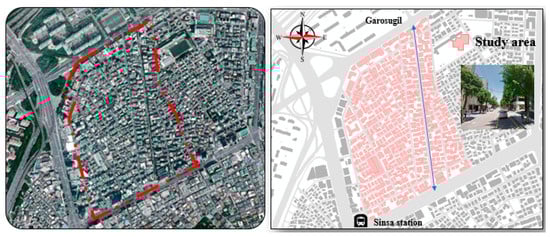
Figure 1.
The study area.
The left image of Figure 1 shows the entire community of Sinsa-dong, which is a neighborhood in Gangnam District, and the arrow in the right image of Figure 1 indicates the center of Garosu-gil, which is the area’s main thoroughfare and the location of most of its commercial amenities. The community was originally formed by an influx of poor artists and young fashion designers and was characterized by a mix of residential and commercial areas; however, in more recent years, most of the residences have been converted for commercial use. Since the displacement of people and places, commercial amenities have been expanded to the west and east, and the community’s original identity as a culturally oriented street has significantly changed over time.
2.1.2. Developing a Schematic Diagram and Data Collection
This research proposed three main stages to explore, investigate, visualize, and predict commercial gentrification in the area of interest (Figure 2).
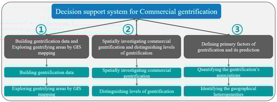
Figure 2.
Schematic diagram to explore, investigate, visualize, and predict commercial gentrification.
As illustrated in the first column of Figure 2, this research began with building a GIS database to explore gentrifying buildings and parcels and visually represent spatial pattern of shifting types and uses of businesses. The resultant outputs can be used for policy decision-making related to gentrifying areas.
Second, as depicted in the middle column of Figure 2, this study identified factors associated with commercial gentrification and analyzed related hot and cold spot trends to determine the levels (degrees) of commercial gentrification. Third (Figure 2, column 3), the study conducted Pearson’s correlation coefficient (hereafter, referred to as ‘correlation’) and regression analyses to quantify the strength of the linear relationship between paired variables associated with primary factors contributing to commercial gentrification. Finally, GWR was used to predict spatial relationships and identify geographical heterogeneities between variables associated with commercial gentrification []. The following sections elucidate the detailed working processes and methodologies proposed in the above schematic diagram.
2.2. Stage 1: Building Gentrification Data and Exploring Gentrifying Areas with GIS Mapping
In order to explore gentrifying areas and buildings in the commercial district, this study collected data on changes in store rent prices, total sales amounts, floating populations, franchise rates, uses (types) of businesses, closure and opening of business, duration of business operation, and length of residence from 2012 to 2017. All values were inserted as vector data in building units and parcels. Table 1 shows the components of the resulting GIS database.

Table 1.
Geographic information system (GIS) database (DB) to explore gentrifying areas.
This study used a road view (commonly known as street view) to depict the historical information of small business. A street view enables the investigation of changes in building appearance, surrounding objects, and types of businesses []. As listed in Table 1, officially assessed land prices and other detailed building information associated with commercial gentrification were incorporated into the GIS database.
2.3. Stage 2: Spatially Investigating Commercial Gentrification and Distinguishing Levels of Gentrification
In stage two, the study used four factors to investigate spatial patterns of commercial gentrification and to distinguish levels of gentrification, and data to analyze gentrifying buildings were collected from 2013 to 2017. Equation (1) was applied to identify changes in store types and thereby assess levels of gentrification according to each of the following four questions (i.e., factors):
- Have residential uses been converted to commercial uses?
- Have commercial amenities (e.g., cafés, restaurants, and clothing, miscellaneous, or cosmetics stores) been altered to other types or purposes?
- Has a general business been switched to a franchise business?
- Were closure rates of business increased?
As shown in Equation (1), we temporally assigned different weights to each of the four factors. Based on the above questions, 0 denotes no change, and 1 is assigned when an alteration has occurred. The weights assigned to the variables depend on their level of importance. Accordingly, has the highest weight because it is one of the major reasons invoking gentrification, has the second highest weight because it indicates that the native businesspersons (i.e., artists) have left the commercial district, and is weighted to the lowest value because the transformation to a franchise business is already considered in . Gentrification level, ‘’, is used to distinguish four levels of commercial gentrification, such that level 1 ranges from 0 to 0.25, level 2 from 0.251 to 0.5, level 3 from 0.51 to 0.75, and level 4 from 0.751 to 1.
As introduced above, the weights of independent variables were temporally determined. However, such weighting is supported by the gentrification literature that focuses on commercial neighbor change. Chapple and Sullivan stated alteration of business types are considered as primary indicators [,,]. It means commercial amenities play key roles in invoking gentrification. In addition to that, this phenomenon finally results in increasing business closing rates. Accordingly, it is considered as second highest weight in this study. Glass also mentioned that as transformation of native working classes goes on, the social and economic character of the district is changed []. It means that changes in social and economic characters are related to the alternation from residential uses to commercial uses. For the reasons, we assigned more weight to the length of residence than the change to a franchise business.
2.4. Stage 3: Defining Primary Factors of Gentrification and Its Prediction
In stage three, correlation and regression analysis were used to determine primary factors causing commercial gentrification, and spatial patterns of the factors were analyzed to predict gentrifying buildings. Three categories were used for the factor analysis: (1) ‘building types and uses’, (2) ‘transportation and roads’, and (3) ‘shopping centers’. The three categories were subdivided into 11 variables, for which use the study considered the following information. First, we examined the changes of the building type and business closures and reopening information as provided by the Seoul Social Economy Center. Second, because gentrified areas generally are clustered and formed near Garosu-gil (the main road), the study considered the proximity of commercial buildings or stores to primary and secondary roads in the study area. Third, changes in store rent prices were used as one of the factors. The first category, ‘building types and uses’, incorporated four variables, namely, ‘single house (SH)’, ‘neighborhood convenience facilities (NCF)’, ‘alteration of building use (ABU)’, and ‘building age (BA)’. The second category included three variables, namely, ‘store rent (SR)’, ‘new franchise businesses (NFB)’, and ‘new restaurant businesses (NRB)’. The third category contained four variables, namely, ‘distance to subways (DS)’, ‘next to secondary roads (NSR)’, ‘having more than two roads (HTR)’, and ‘close to the main road (CMR)’. As stated in Section 2.3, the above variables are mostly supported by the gentrification literature that focuses on the commercial neighbor change. For example, as for the first category, the ideas are from the indicators used in Chapple and Sullivan’s studies [,]. Regarding the second category, Smith stated about the capitalized ground rent and sale price, and Ley also argued about dwelling values [,,]. Regarding the third category, the variable with the distance-decay effect is supported by the study of Bruechner and Rosenthal [].
Next, correlation and regression analyses were used to quantify associations between paired variables as related to commercial gentrification []. GWR was used to predict the variables’ spatial relationships and identify the geographical heterogeneities between them, after which the spatial pattern was compared with the results of hot spot analysis. The hot spot analysis used Getis-Ord Gi* statistics to identify statistically significant clustering of gentrification factors with high values or low values [,]. The level of significance was established at the 95% confidence interval.
3. Results
3.1. Exploring the Gentrification Phenomenon
3.1.1. Mapping Gentrification Data
As demonstrated in Table 1, this research collected and built GIS databases containing variables associated with gentrification.
As shown in Figure 3a, the majority of the buildings in the area were built between 1968 and 1983. Many of those are decrepit. A number of the structures along Garosu-gil’s main road were rebuilt between 2006 and 2014. Moreover, a number of the buildings in the residential area have been converted to commercial facilities (a rectangle box in Figure 3b). Interestingly, some portions in the district are classified as detached dwelling and cultural facilities (Classes 1 and 2 in Figure 3c).
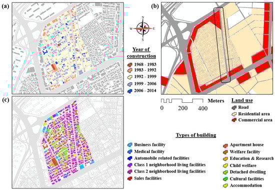
Figure 3.
Mapping for years of building construction (a), types of land use (b), and types of buildings (c).
3.1.2. General Status of Gentrification-Related Variables
The following shows Changes in officially announced standard land price and store rent costs between 2012 and 2017. As shown in Figure 4, the officially announced standard land price (OASLP) in the study area has increased by about 1.5 times (from 600 to 980) (a-1), which is more than the corresponding increases in Seoul as a whole. Store rental fees increased in every year of the study period, except for 2013 and 2017, and such increases are much higher than those in Seoul as a whole (b-2).
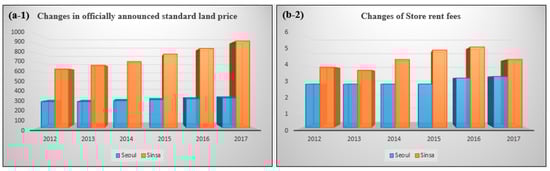
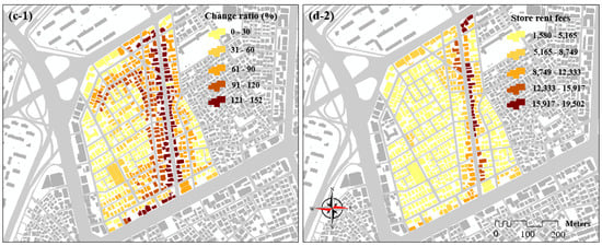
Figure 4.
Changes in officially announced standard land price and store rent costs between 2012 and 2017.
The highest rates of OASLP changes are represented along Garosu-gil’s main street. Although the highest store rental fees are similarly clustered along Garosu-gil road, the buildings with the largest price increases extend to neighboring alleys. Many large cosmetic stores are located along the street itself, whereas restaurants tend to be clustered in alleys. The current structure of commercial amenities has led to rent increases for stores that cater to the floating population, such that native small businesses and artists have been pushed out of the district. The decreasing store rents in 2016 represent an anomaly: that year saw a dramatic decline in the number of tourists due to political issues concerning the defense of terminal high-altitude areas.
Figure 5 shows the total sale amounts and floating population in 2017.
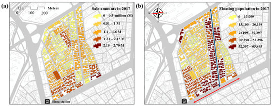
Figure 5.
Total sale amounts (a) and floating population in 2017 (b).
The pattern of store sales and floating population locations clearly indicates that the buildings are gentrified. Stores located along the center of the Garosu-gil road had total sales ranging from $8700 (10 million won [KRW]) to $14,000 (16 million won [KRW]) in 2017 (Blue arrow in Figure 5a), whereas sales for stores located next to Sinsa station range from $14,000 to $23,400 (28 million won [KRW]) (Red arrow in Figure 5a). The majority of the floating population was clustered near Garosu-gil’s main thoroughfare and stores near Sinsa station.
Figure 6 shows changes in commercial amenities from 2012 to 2017.

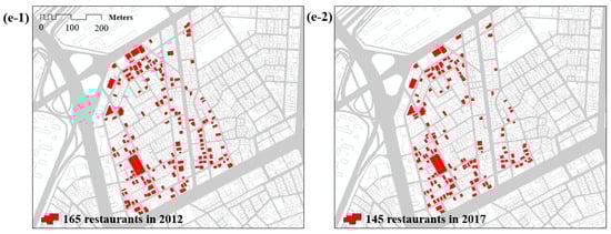
Figure 6.
Alteration of business types from 2012 to 2017: cosmetic stores (a-1,a-2); bakery stores and coffee shops (b-1,b-2); clothing and grocery stores (c-1,c-2); convenience stores (d-1,d-2); and restaurants (e-1,e-2).
As shown in Figure 6(a-1,a-2), cosmetic stores represent the greatest area of new business investments. The number of cosmetic stores increased threefold over 5 years from 2012 to 2017, and the number of clothing stores increased nearly twofold during the same period Figure 6(c-1,c-2). The growth of convenience stores was slightly more modest at nearly 35% Figure 6(d-1, d-2). In contrast, the number of bakery stores and coffee shops slightly decreased, and there was a 12% decrease in restaurants Figure 6(b-1,b-2). The decrease in restaurants began after 2013 Figure 6(e-1,e-2), whereas that in bakery stores began in 2015.
The expansion of new businesses into residential areas is considered a key factor in explaining processes of rapid commercial gentrification. As Figure 7 illustrates, the speed of business closure far exceeded that of business openings; whereas the number of new businesses grew by 130%, closures increased by 329% from 2012 to 2017 Figure 7(a-1,a-2).
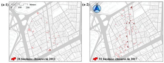
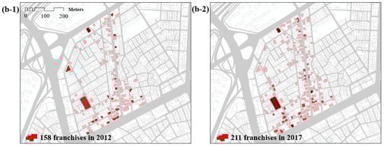
Figure 7.
Closed stores (a-1) in 2012 and (a-2) in 2017 and opened new businesses (b-1) in 2012 and (b-2) in 2017.
As of 2017, most closed stores were located near Sinsa station and the main street, whereas new franchises in 2012 and 2017 were clustered near both places as well as in residential areas.
Figure 8a depicts the duration of business operations. Most stores had operated for 2 or 3 years (a-1,a-2). By 2014, only approximately 20% of businesses had been opened over 5 years; however, the number of stores had decreased to only ten stores by 2016, which indicates the closure of many long-operating businesses.
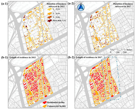
Figure 8.
Durations of business operation (a-1,a-2) and lengths of residence (b-1,b-2) for residential and commercial facilities.
During the study period, a number of commercial facilities have expanded to alleys near Garosu-gil’s main street (rectangular box in b-2); however, there were only small differences in lengths of residence between 2012 and 2017 (Figure 8(b-1,b-2)). The red color indicates residential facilities and yellow illustrates commercial facilities.
3.2. Spatially Investigating Commercial Gentrification and Distinguishing Levels of Gentrification
3.2.1. Spatially Investigating Commercial Gentrification
As introduced in Section 3.3, four questions were used to identify and spatially investigate gentrifying buildings. As shown in Figure 9, there were annual increases in the number of commercial facilities, such as convenience stores and new franchise-style businesses during the study period, whereas business closures and new convenience stores decreased in 2017.
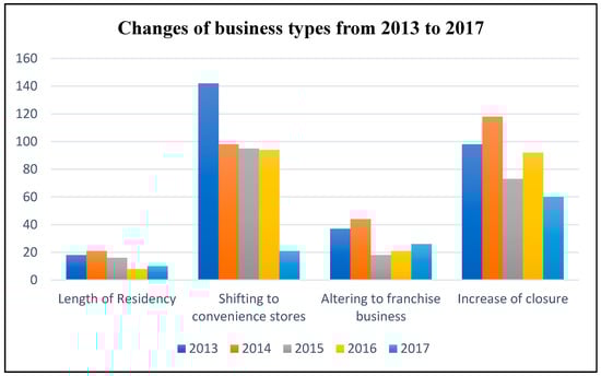
Figure 9.
Changes of business types from 2013 to 2017.
Based on the information depicted in Figure 9 and Figure 10, it appears that the process of commercial gentrification had begun before 2013. This study associated the four factors listed therein with buildings contributing to commercial gentrification. Figure 10 depicts the number of buildings affected by the four factors from 2013 to 2017 and shows those that have become highly gentrified over time.
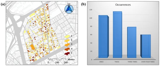
Figure 10.
Counts of gentrifying buildings (How often were buildings gentrified from 2013 to 2017?): (a) the number of gentrified commercial building, (b) the number of stores experienced alteration of business type.
Simply speaking, larger numbers associated with the buildings in Figure 10 indicate a more accelerated commercial gentrification process. As shown in Figure 10a, most buildings are counted more than twice. Figure 10b shows that many stores were altered to other types of businesses from 2013 to 2017. Approximately 150 stores experienced three to four shifts to other businesses during this period.
Next, this study analyzed hot and cold spot trends of the gentrified buildings accumulated in Figure 10. In 2013 (Figure 11a), the northwestern and southeastern zones of the study area were statistically significant hot spot areas with high values of gentrified buildings. The clustered patterns intensify near Garosu-gil’s main road, and the significant hot spots had expanded to the middle of the main road by 2014–2015 (Figure 11b,c), thus indicating an acceleration of the gentrification process. In 2016, the hot spot pattern is similar with that in 2013 (Figure 11d). In 2017, the buildings near the Sinsa station and southeastern areas show hot spot trends with the high number of gentrified buildings (Figure 11e). Accordingly, the gentrification pattern was centered on the Garosu-gil district. It was most intense in the district.
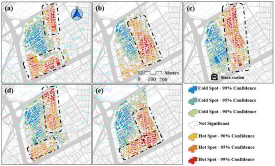
Figure 11.
Hot spot trends of gentrified buildings: (a) 2013; (b) 2014; (c) 2015; (d) 2016; (e) 2017.
As introduced before, the hot spot analysis can identify statistically significant clustering of variables with high (red zones) or low (blue zones) values. It begins by identifying a null hypothesis, and thereby z-scores and p-values returned by the method tell if we can reject the null hypothesis or not. As a result, the resultant outputs above exhibit significant clustering rather than a random pattern (premising complete null hypothesis). To reject the null hypothesis, the method uses three confidence levels at 90 (p < 0.1), 95 (p < 0.05), or 99 (p < 0.01) percent. For example, with a confidence level of 99 percent, it indicates we are unwilling to reject the null hypothesis (presuming random patterns) because it would be less than a 1 percent probability to tell a random pattern. Thus, Figure 11 shows clustering of gentrification factors with high and low values at three confidence levels.
3.2.2. Distinguishing Levels of Gentrification
In the next stage of analysis, the study attempted to identify levels of commercial gentrification. Higher values of y in Equation (1) indicate the existence of more gentrified buildings. Each of the four questions was assigned different weights, and commercial gentrification was subdivided into four levels.
Figure 12 shows outputs resulting from Equation (1) from 2013 (a) to 2017 (e). As introduced in Section 3.3, level 1 ranges from 0 to 0.25, level 2 from 0.251 to 0.5, level 3 from 0.51 to 0.75, and level 4 from 0.751 to 1. Level 4 indicates that areas or buildings are highly gentrified. The five maps with the four levels of commercial gentrification demonstrate a wide spatial distribution of commercial gentrification in the study area. Moreover, the gentrification levels in Garosu-gil are much higher than in the rest of Sinsa-dong (Figure 12f). The levels of gentrification are moderated from 2013 (a) to 2017 (e).
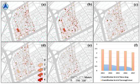
Figure 12.
Results of the gentrification assessment levels: (a) 2013; (b) 2014; (c) 2015; (d) 2016; (e) 2017.
3.3. Investigating Primary Factors of Gentrification and Its Prediction
3.3.1. Results of Correlation and Regression Analyses
As described in Section 2.1.2, correlation analysis was used to determine associations between pairs of gentrification variables. The values for y, ‘gentrification level’, computed in Section 3.2.2, were used as independent variables, and there were 11 dependent variables.
Table 2 shows the results of the correlation analysis. Neighborhood convenience facilities (NCF), building ages (BA), store rents (SR), new franchise businesses (NFB), new restaurant businesses (NRB), distance to subways (DS), and having more than two roads (HTR) have positive correlations with commercial gentrification. Among these, SR and NRB have more moderate positive relationships than other variables. In contrast, single house (SH) has a negative correlation and is not directly associated with commercial gentrification.
Table 2.
Correlation coefficients (CC) and p values between pairs of variables.
3.3.2. Results of Regression Analysis
Regression analysis was used to identify the gentrification’s association between ‘y’ and the following variables. We excluded alteration of building use (ABU) from the analysis because the related data were intermittently reported to authorities having jurisdiction over business owners and thus are less reliable. In addition, location next to secondary roads (NSR) was excluded because it had no correlation with the independent variable.
As shown in Table 3, the results of NCF, NFB, NRB, and CMR are statistically significant, whereas SH, BA, SR, DS, and HTR have relatively little explanation in terms of the gentrification’s association. In general, ordinary least squares linear regression enables to quantify the strength of the linear relationship between pairs of variables associated with primary factors contributing to commercial gentrification. Such model is used not only to predict future patterns that help explore spatial relationship, but also to predict global model for the variable we are trying to understand.
Table 3.
Results of regression analysis.
Along with that, we also examined the variance inflation factor (VIF) values to reflect how much redundancy among the model explanatory variables can be biased. If all predictors were less than 2, it indicates there were no multicollinearity problems among the explanatory variables. If the VIF value is greater than 10, it indicates that multicollinearity existed []. Ideally, the smaller is definitely better. The following Table 4 shows VIF values from 2013 to 2017.
Table 4.
Variance inflation factor (VIF) values from 2013 to 2017.
As a result, multicollinearity was assessed to check for redundancy among the four explanatory variables. The VIF values range from 1.05 to 2.43 during the 5 years. In particular, the VIF values of NCF, NFB, NRB, and CMR are between 1.04 and 2.36. It indicates that none of the variables are redundant.
In addition to that, this study is interested in predicting spatial relationships between significant variables (NCF, NFB, NRB, and CMR). Thus, in the following step, a geographically weighted regression (GWR) model is used to look for geographical differences and spatial variation in the relationship between the dependent variable and the independent variables. The method event provides a local model of the dependent variable to be explained. For that reason, GWR was applied to identify and predict spatial relationships between pairs of variables.
3.3.3. Results of GWR
Whereas simple linear regression models can examine only single stationary coefficients of each independent variable, GWR identifies variations between coefficients of independent variables (i.e., heterogeneity) in terms of their magnitude and direction [,]. Thus, GWR can identify where spatial associations of gentrification variables exist (hot zones) or are absent (cold zones), and thereby it is possible to find areas where the independent variables have a positive and negative relationship with the dependent variable. In this analysis, y was used as an independent variable, and the average of the regression coefficients was used as a dependent variable.
As Figure 13 illustrates, the adjusted R-squared value ranged from 0.69 in 2013 to 0.58 in 2017. The adjusted R-squared value is a modified version of R-squared value. R-squared tells how much of the variation in the dependent variable has been explained by the model. When comparing with modified R-squared of the regression model, all values are increased. R-squared is a measure of goodness of fit and its value ranges from 0.0 to 1.0, with higher values being desirable. In general, if R-squared value is over 0.7, this value is generally considered strong effect size, but depends on what we are modelling [].
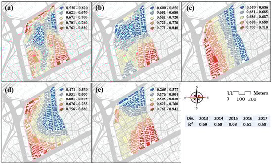
Figure 13.
Mapping of the locally weighted coefficients of determination (R2): (a) 2013; (b) 2014; (c) 2015; (d) 2016; (e) 2017.
As shown in Figure 13, GWR allows us to map gentrification levels (y). In 2013 (a), positive relationships were mostly clustered in the southeastern areas and near Apgujeong-ro (west and east) and Dosan-daero; whereas in 2014 (b), the predictive patterns with positive relationship were clustered only in the southeastern area, and in 2015 (c), positive relationships were clustered only near Sinsa station and Apgujeong-ro (north and south, respectively). In 2016 (d), the positive patterns were clustered near Sinsa station, Apgujeong-ro (north and south and west and east directions), and Dosan-daero; however, in 2017 (e), the positive relationships were again clustered in the southeastern area.
4. Discussion
Gentrification is a growing concern in urban areas. As stated in the introduction, the gentrification process is an inevitable social phenomenon because people run businesses with the aim to earn profits. The process begins with changes in the commercial characteristics of neighborhoods and eventually extends to negatively impact the original working-class residents, as rental and living costs begin to exceed their means. As stated in the Introduction section, even though a number of gentrification studies have been conducted over the years, it is challenging to collect reliable datasets or statistical maps which can be used by urban planners and policymakers to implement preventative or supportive programs for the native working classes or artists. Furthermore, the wide range of gentrification studies have been focused on at the neighborhood levels, and comparatively limited research has explicitly focused on this phenomenon at finer spatial scales, such as neighborhood parcels, building units, or 3D.
Regarding the concerns on previous work, this research developed a comprehensive research approach to provide policymakers with standardized and quantified criteria to help identify the stages of gentrification and protect cultural artists and small businesspersons from the negative outcomes of this process. The study developed three main steps to explore, investigate, visualize, and predict commercial gentrification in the area of interest. Specifically, multiple data sources associated with commercial gentrification were first collected and built into GIS databases, which were used to explore gentrifying buildings. Second, the study investigated buildings affected by commercial gentrification and distinguished levels of commercial gentrification. To spatially investigate commercial gentrifications, four questions (factors) were integrated into a gentrification level variable (y), which was subdivided into four levels of commercial gentrification, which can be used for administrative purposes in several scenarios. For example, at the first level (ranging from 0 to 0.25) denoting the initial state of gentrification, public officers can gather local community groups at public hearing sessions or conferences. At the second level (0.2561–0.50), public officers need to engage in reasonable mutual exchanges of opinions and ideas between building owners, store renters, and local authorities and develop preventive programs. At the third level of gentrification, the local authority can begin restricting or adjusting to new businesses and develop measures to protect the interests of all stakeholders. At the last level, when lower-income renters have become disadvantaged, the local authorities should devise means to provide financial or administrative supports to those renters. Furthermore, hot spot trends of gentrified buildings were mapped, which revealed that the gentrification process is primarily clustered near Garosu-gil and Sinsa station and has expanded to alleys along Garosu-gil’s main street. It is evident that shifts in the local cultural economy have transformed Garosu-gil’s characteristics and created commercially gentrified areas. As a result, smaller businesses are disappearing, and the cultural artists initially involved in growing Garuso-gil’s community are being pushed out as rental fees increase. Residential areas are being reduced while commercial areas are expanding, with the result being the gradual disappearance of the original regional characteristics initially formed by cultural artists.
In sum, the contributions of the study are as follows. First, the predictive spatial mappings produced in this study can be used for policymakers to properly help areas suffering from gentrification issues. For example, based on the 2014 map (Figure 13b) and spatial patterns of the red zones over time, public officers in the jurisdiction can go to the buildings in red zones and then investigate or explore how much the buildings are suffering from the issues. The method resulting in the GWR maps can enable scientists and urban planners to visualize gentrification levels heterogeneously and spatially across the study area.
Second, this research contributes to the development of valuable datasets and criteria to aid policymakers in enhancing the sustainability of the gentrification process by providing more support and services to affected communities, as well as planning and implementing future national urban renewal projects.
This research has two main limitations. Firstly, our results are based on publicly available data and private data owned by companies, as we encountered difficulties in collecting rental fees and total sale amounts due to privacy issues. Second, although this research used the finest possible spatial scale, which is a building unit, such structures often comprise multiple stories and businesses. Below shows an example of identifying gentrification levels in 3D.
In general, the range of rental costs is affected by what level their store is located and a type of business. In this study we temporally analyzed a building to identify a gentrification level in 3D. Figure 14 briefly expands the building level analysis to model a four-story building containing multiple businesses. The 3D map in the left of Figure 14 represents hot and cold spot trends of commercial gentrification, and the right thing in Figure 14 shows vertically represented hot and cold spot trends in a single building. This model can directly assist stores suffering from gentrification issues with the four assessment levels developed in this research.
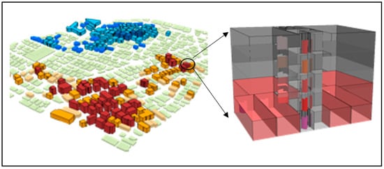
Figure 14.
3-D representation of commercial gentrification and hot spot trends in 3D.
5. Conclusions
Since the term ‘gentrification’ was coined in 1964 by Glass, the term has been expanded by many sociologists. Nowadays, gentrification is a widely known phenomenon for the general public. As ever, the process of gentrification is nationally occurring around the world. The phenomenon was unavoidable in multiple places in South Korea. Residents near Garosu-gil have faced multi-faceted problems such as rapid increase of housing and rental costs. The character of Garosu-gil neighborhoods is changing rapidly and the original native working classes are pushed out from increasing rents. This concludes that displacement disproportionately impacts communities of the artist-residencies and local cultural economy. We note that this research is focused on spatially characterizing and exploring the commercial gentrification phenomenon at Garosu-gil. This study also examined gentrification issues per building with at the finest spatial scales in 2D and 3D. The resultant outputs are visually and spatially quantified over time that are stored in GIS database. This research will be beneficial for urban planners or policy makers who pursue sustainable urban development, particularly for the original working-classes at an artist-resident community area. Ultimately, this study helps urban planners implement future national urban renewal projects to protect low-income residents and small businesses and in so doing stimulate more sustainable community development. In future studies, we will develop more detailed vertical representations to analyze commercial gentrification more accurately.
Author Contributions
B.Y., J.P. and J.K. developed the theory and performed the computation, in addition to verifying the analytical methods and writing this paper. All authors participated in this research project to design, review, assess, and write this paper. All authors have read and agreed to the published version of the manuscript.
Funding
No funding.
Acknowledgments
This work was supported by the Dongguk University Research Fund of 2019.
Conflicts of Interest
No potential conflict of interest is reported by the authors.
References
- Glass, R. Introduction to London: Aspects of Change; Centre for Urban Studies: London, UK, 1964. [Google Scholar]
- Marcuse, P. Comment on Elvin, K. Wyly and Daniel, J. Hammel’s “Islands of Decay in Seas of Renewal: Housing Policy and the Resurgence of Gentrification”. Hous. Policy Debate 1999, 10, 789–797. [Google Scholar] [CrossRef]
- Smith, N. Gentrification and the rent gap. Ann. Assoc. Am. Geogr. 1987, 77, 462–465. [Google Scholar] [CrossRef]
- Lim, H.; Kim, J.; Potter, C.; Bae, W. Urban regeneration and gentrification: Land use impacts of the Cheonggye Stream Restoration Project on the Seoul’s central business district. Habitat Int. 2013, 39, 192–200. [Google Scholar] [CrossRef]
- Patch, J. The embedded landscape of gentrification. Vis. Stud. 2004, 19, 169–187. [Google Scholar] [CrossRef]
- Zukin, S. Loft Living: Culture and Capital in Urban Change; Rutgers University Press: New Brunswick, NJ, USA, 1989. [Google Scholar]
- Kim, J. Cultural entrepreneurs and urban regeneration in Itaewon, Seoul. Cities 2016, 56, 132–140. [Google Scholar] [CrossRef]
- Yoon, Y.; Park, J. Stage classification and characteristics analysis of commercial gentrification in Seoul. Sustainability 2018, 10, 2440. [Google Scholar] [CrossRef]
- Hong, H.; Koo, J. Commercial cluster characteristics in residential district focusing on Garosu Street. J. Cadastre Land Inf. 2016, 46, 57–77. [Google Scholar]
- Curley, G. Gallery: ‘Europe in Seoul’ on Garosugil Street. 2010. Available online: http://travel.cnn.com/explorations/life/gallery-europe-seoul-garosugil-street-043125/ (accessed on 21 June 2020).
- Lees, L.; Slater, T.; Wyly, E.K. Gentrification; Routledge: London, UK, 2013. [Google Scholar]
- Smith, N. The New Urban Frontier: Gentrification and the Revanchist City; Psychology Press: London, UK, 1996. [Google Scholar]
- Lees, L. The geography of gentrification: Thinking through comparative urbanism. Progress Hum. Geogr. 2012, 36, 155–171. [Google Scholar] [CrossRef]
- Zukin, S. The Cultures of Cities; Wiley: Hoboken, NJ, USA, 1996. [Google Scholar]
- Chapple, K.; Jacobus, R. Retail trade as a route to neighborhood revitalization. Urban Reg. Policy Effects 2009, 2, 19–68. [Google Scholar]
- Freeman, L. There Goes the Hood: Views of Gentrification from the Ground Up; Temple University Press: Philadelphia, PA, USA, 2011. [Google Scholar]
- Sullivan, D.M.; Shaw, S.C. Retail gentrification and race: The case of Alberta Street in Portland, Oregon. Urban Aff. Rev. 2011, 47, 413–432. [Google Scholar] [CrossRef]
- Zukin, S. Naked City: The Death and Life of Authentic Urban Places; Oxford University Press: Oxford, UK, 2009. [Google Scholar]
- Zuk, M.; Bierbaum, A.H.; Chapple, K.; Gorska, K.; Loukaitou-Sideris, A.; Ong, P.; Thomas, T. Gentrification, Displacement and the Role of Public Investment: A Literature Review; Federal Reserve Bank: San Francisco, CA, USA, 2015; p. 32. [Google Scholar]
- NIAS. Market Generated Displacement: A Single City Case Study; National Institute for Advanced Studies: Washington, DC, USA, 1981. [Google Scholar]
- Charles, C.Z. Neighborhood racial-composition preferences: Evidence from a multiethnic metropolis. Soc. Probl. 2000, 47, 379–407. [Google Scholar] [CrossRef]
- Ellen, I.G.; Horn, K.; O’Regan, K. Pathways to integration: Examining changes in the prevalence of racially integrated neighborhoods. Cityscape 2012, 14, 33–53. [Google Scholar]
- Hipp, J.R. Segregation through the lens of housing unit transition: What roles do the prior residents, the local micro-neighborhood, and the broader neighborhood play? Demography 2012, 49, 1285–1306. [Google Scholar] [CrossRef] [PubMed][Green Version]
- Marcuse, P. Abandonment, gentrification, and displacement: The linkages in New York City. In Gentrification of the City; Smith, N., Williams, P., Eds.; Routledge: Abingdon, UK, 2013; pp. 153–177. [Google Scholar]
- Newman, S.J.; Owen, M.S. Residential displacement: Extent, nature, and effects. J. Soc. Issues 1982, 38, 135–148. [Google Scholar] [CrossRef]
- Schill, M.H.; Nathan, R.P.; Persaud, H. Revitalizing America’s Cities: Neighborhood Reinvestment and Displacement; Suny Press: Albany, NY, USA, 1983. [Google Scholar]
- O’Sullivan, D. Geographical information science: Critical GIS. Prog. Hum. Geogr. 2006, 30, 783–791. [Google Scholar] [CrossRef]
- Parker, C.; Pascual, A. A voice that could not be ignored: Community GIS and gentrification battles in San Francisco. In Community Participation and Geographic Information Systems; Craig, W.J., Harris, T.M., Weiner, D., Eds.; Taylor and Francis: Oxfordshire, UK, 2002; pp. 55–64. [Google Scholar]
- Chapple, K. Mapping Susceptibility to Gentrification: The Early Warning Toolkit; Center for Community Innovation: Berkeley, CA, USA, 2009. [Google Scholar]
- Chipman, J.; Wright, R.; Ellis, M.; Holloway, S.R. Mapping the evolution of racially mixed and segregated neighborhoods in Chicago. J. Maps 2012, 8, 340–343. [Google Scholar] [CrossRef]
- Greene, R.P.; Pick, J.B. Exploring the Urban Community: A GIS approach; Prentice Hall: Upper Saddle River, NJ, USA, 2012. [Google Scholar]
- Kwon, Y.; Joo, S.; Han, S.; Park, C. Mapping the distribution pattern of gentrification near urban parks in the case of Gyeongui Line Forest Park, Seoul, Korea. Sustainability 2017, 9, 231. [Google Scholar] [CrossRef]
- Maantay, J.; Maroko, A.R. Brownfields to greenfields: Environmental justice versus environmental gentrification. Int. J. Environ. Res. Public Health 2018, 15, 2233. [Google Scholar] [CrossRef]
- Crooks, A.T. Constructing and implementing an agent-based model of residential segregation through vector GIS. Int. J. Geogr. Inf. Sci. 2010, 24, 661–675. [Google Scholar] [CrossRef]
- Jackson, J.; Forest, B.; Sengupta, R. Agent-based simulation of urban residential dynamics and land rent change in a gentrifying area of Boston. Trans. GIS 2008, 12, 475–491. [Google Scholar] [CrossRef]
- Torrens, P.M.; Nara, A. Modeling gentrification dynamics: A hybrid approach. Comput. Environ. Urban Syst. 2007, 31, 337–361. [Google Scholar] [CrossRef]
- Yin, L. The Dynamics of Residential Segregation in Buffalo: An Agent-Based Simulation. Urban Stud. 2009, 46, 2749–2770. [Google Scholar] [CrossRef]
- Eckerd, A.; Kim, Y.; Campbell, H. Gentrification and displacement: Modeling a complex urban process. Hous. Policy Debate 2019, 29, 273–295. [Google Scholar] [CrossRef]
- Liu, C.; O’Sullivan, D. An abstract model of gentrification as a spatially contagious succession process. Comput. Environ. Urban Syst. 2016, 59, 1–10. [Google Scholar] [CrossRef]
- Galea, S.; Ettman, C.K.; Vlahov, D. The Present and future of cities. In Urban Health; Oxford University Press: Oxford, UK, 2019; p. 1. [Google Scholar]
- Phillis, Y.A.; Kouikoglou, V.S.; Verdugo, C. Urban sustainability assessment and ranking of cities. Comput. Environ. Urban Syst. 2017, 64, 254–265. [Google Scholar] [CrossRef]
- Brunsdon, C.; Fotheringham, A.S.; Charlton, M.E. Geographically weighted regression: A method for exploring spatial nonstationarity. Geogr. Anal. 1996, 28, 281–298. [Google Scholar] [CrossRef]
- Lee, K.; Lee, S.; Jung, W.; Kim, K. Fast and accurate visual place recognition using street-view images. ETRI J. 2017, 39, 97–107. [Google Scholar] [CrossRef]
- Ley, D.; Tutchener, J.; Cunningham, G. Immigration, polarization, or gentrification? Accounting for changing house prices and dwelling values in gateway cities. Urban Geogr. 2002, 23, 703–727. [Google Scholar] [CrossRef]
- Brueckner, J.K.; Rosenthal, S.S. Gentrification and neighborhood housing cycles: Will America’s future downtowns be rich? Rev. Econ. Stat. 2009, 91, 725–743. [Google Scholar] [CrossRef]
- Getis, A.; Ord, J.K. The analysis of spatial association by use of distance statistics. Geogr. Anal. 1992, 24, 189–206. [Google Scholar] [CrossRef]
- Ord, J.K.; Getis, A. Local spatial autocorrelation statistics: Distributional issues and an application. Geogr. Anal. 1995, 27, 286–306. [Google Scholar] [CrossRef]
- Mason, R.L.; Gunst, R.F.; Hess, J.L. Statistical Design and Analysis of Experiments: With Applications to Engineering and Science; John Wiley & Sons: Hoboken, NJ, USA, 2003; p. 760. [Google Scholar]
- Fotheringham, A.S.; Charlton, M.E.; Brunsdon, C. Geographically weighted regression: A natural evolution of the expansion method for spatial data analysis. Environ. Plan. A 1998, 30, 1905–1927. [Google Scholar] [CrossRef]
- Yang, B.Y.; Hwang, C.S. Spatial dependency and heterogeneity of adult diseases: In the cases of obesity, diabetes and high blood pressure in the USA. J. Korean Assoc. Reg. Geogr. 2010, 16, 610–622. [Google Scholar]
- Moore, D.S.; Notz, W.I.; Flinger, M.A. The Basic Practice of Statistics, 6th ed.; Freeman and Company: New York, NY, USA, 2013; p. 138. [Google Scholar]
© 2020 by the authors. Licensee MDPI, Basel, Switzerland. This article is an open access article distributed under the terms and conditions of the Creative Commons Attribution (CC BY) license (http://creativecommons.org/licenses/by/4.0/).