Article

Creating a Comprehensive Method for the Evaluation of a Company

1
The Faculty of Operation and Economics of Transport and Communications, University of Zilina, Univerzitna 8215/1, 01026 Zilina, Slovakia
2
School of Expertness and Valuation, Institute of Technology and Business, Okruzni 517/10, 37001 Ceske Budejovice, Czech Republic
*
Author to whom correspondence should be addressed.
Sustainability 2020, 12(21), 9114; https://doi.org/10.3390/su12219114
Submission received: 30 September 2020 / Revised: 29 October 2020 / Accepted: 31 October 2020 / Published: 2 November 2020
(This article belongs to the Special Issue Company Assessment: Basis of Its Sustainable Development)

Abstract

:
For investment purposes, the evaluation of a company is not only a matter for a company itself, but also for shareholders and external persons. There are many methods for evaluating a company. This contribution therefore focuses on the creation of a comprehensive method for the evaluation of an industrial enterprise, one that can be used to predict potential future bankruptcies, using a dataset of financial statements of active companies and those in liquidation in the period 2015–2019. Artificial neural networks were used to process the data, specifically logistic regressions from the data processed in the Statistica and Mathematica software programmes. The results showed that the models created using the Mathematica software are not applicable in practice due to the parameters of the obtained results. In contrast, the artificial neural structures obtained using the neural network model in the Statistica software were prospective due to their performance, which is almost always above 0.8, and the logical economic interpretation of the relevant variables. All the generated and retained networks show excellent performance and few errors. However, one of the artificial structures, network no. 4 (MLP 16-16-2), produces better results than the others. Overall, accuracy is almost 81%. In the case of the classification of companies capable of surviving financial distress, accuracy is almost 90%, with that for the classification of companies at risk of going into bankruptcy at nearly 55%.

1. Introduction

Management decisions, in particular those concerning, among other things, acquisitions and financing, are all directly related to the evaluation of a company. This is why it is a highly popular topic among researchers, as Laaksonen and Peltoniemi [1] show. Companies require a comprehensive assessment that clearly predicts their financial situation in today’s competitive business world. Several studies show that companies that apply the effective use of data and system solutions achieve better results than companies controlled by dominant managerial subjective decision-making [2]. That is why these evaluation methods have gained acceptance by modern companies. Evaluation reports not only provide a comprehensive picture based on financial statements, but also provide a robust basis for decision-making by both the management and, for example, banks [3]. Klieštik et al. [4] states that financial indicators also play an important role in revealing a company’s financial health while helping the company maintain its competitive position and achieve stable development, thereby helping to eliminate potential financial risks.
Devi and Radhika [5] assert that globalization has prompted a more accurate prediction of a company’s financial status because they must provide useful information for stakeholders and the public. A company’s financial profile, as reflected by their financial statements, can make it easier to predict their financial behaviour [6]. Bankruptcy predictions in companies are carried out by utilizing conventional statistical and machine learning methods.
The issues of sustainability and social responsibility are also increasingly being discussed in relation to the evaluation of companies and their financial health. A number of studies and discussions have focused on the potential benefits of such business behaviour compared to the costs of achieving sustainable goals. The most frequently mentioned benefit is the growth of a company’s sustainable performance, due to which the company’s financial health strengthens [7]. Da Costa and Boente [8] agree with this conclusion, stating that the aim of companies is to include all the basic dimensions of sustainable development and to integrate this concept into corporate governance, precisely in order to increase performance. According to Grandhi and Wibowo [9], the concept of sustainability is often seen by companies as a way to gain a competitive advantage and therefore increase their competitiveness. The importance of the sustainability of companies is not questioned by Hawrysz and Maj [10], who believe that this can bring an organization long-term measurable benefits, such as increased investor interest or improved employee and stakeholder loyalty. Lombardo et al. [11] are of the opinion that corporations actively involved in CSR pay attention to the evaluation of all the results of their activities, including well-being. However, a comprehensive and objective assessment of well-being is a very difficult challenge because it is a broad concept involving tangible and intangible elements that change over time.

2. Literature Review

2.1. Neural Network Models

Neural Network (NN) models work very well with regards to bankruptcy prediction, with an average success rate of 81.3785% [12]. Messai and Gallali [13] support their findings in 2015, going on to state that NN models are useful for financial institutions and policy makers. Consequently, Chen [14] is optimistic that Particle Swarm Optimization in conjunction with the Support Vector Machine method can accurately predict bankruptcy. Even when machine learning techniques are only used to support other models, the results show that they outperform other models [15]. Multilayer Perceptron Neural Networks (MLP) have also been proven to perform very well, and better than other techniques, in predicting the capability of construction companies in the Czech Republic to weather a financial crunch [16]. NN models for predicting bankruptcy are qualified, dynamic, and adapt to the financial environment and data availability, as well as outperform discriminant analysis [17]. Despite this, conventional and known bankruptcy prediction models are seen to be relatively accurate [18].

2.2. Company Specific Model

Sayari and Mugan [19] recommended creating company specific bankruptcy prediction models. They further proved that financial relations do indeed boom business features and that information content of specific fractions varies among different industries, diverging impact of industry characteristics on companies. Chen [20], on the contrary, took an alternative approach, and in his opinion a more robust one, choosing not to create a company specific model, but rather combining financial ratio analysis, confirmatory factor analysis and logistic-regression analysis to estimate the probability of the financial failure of public corporations. Alaminos et al. [21] created a global model with a high capacity for bankruptcy prediction. The results they obtained confirm the supremacy of global models in comparison to regional models over periods of up to three years preceding bankruptcy. In all instances, research techniques have shown some significant differences in the process of model creation, as well as in the attained results [21]. According to Hu and Sathye [22], a model that incorporates company-specific money related factors, company-specific non-budgetary factors, and a large-scale monetary variable is a superior indicator of fiscal misfortune than a model that incorporates just the primary arrangement of factors or a model that incorporates the last two arrangements of factors in the Hong Kong growth enterprise markets. Future research involving the use of the Apache Mahout Tool may improve bankruptcy prediction because it enables the integration of evolutionary algorithms with machine learning methods [5]. Managers should be able to recognize the signals of financial failure in advance and comprehend future progression trends; hence, the financial path prediction model can be an active boost to the research field of financial catastrophe analysis and prediction [6]. Vochozka [23] adds that it is necessary for a company to be assessed in terms of its financial situation at each stage of its development. There are a lot of options. An analysis of financial indicators and various comparison methods can be used. From the point of view of interpretation, it seems advantageous to use comprehensive evaluation methods.
In general, there are a number of applications, as well as the emergence of new predictive models based on, for example, the training autoregressive model of recurrent neural networks [24]. Lei [25] presents a predictive model for assessing the quality of a society’s decision-making process based on deep learning algorithms. Hybrid models of neural networks used to predict financial performance based on a comparison of five methods are preferred by Khashei and Hajirahimi [26]. Neural networks for calculating the elasticity of a company’s ability to neutralize financial risk in relation to systemic risk factors are used in the Ukrainian environment by Kolupaieva et al. [27].
Lohmann and Ohliger [28] answer the very question of whether the evaluation of the bankruptcy prediction model should take into account the total cost of misclassification with a positive result. Gulsoy and Kulluk [29] point out the need to take into account differences in the size of a company and therefore the need for adjustments to the evaluation methods. The same authors also focus on the evaluation of mutual funds using the fast adaptive neural network classifier (FANNC) [29]. Atsalakis [30] focuses specifically on the area of emission allowance prices, creating a model based on computational intelligence techniques for their prediction, including a hybrid neurofusion controller which forms a closed-loop feedback mechanism; an artificial neural network system (ANN) and an adaptive inference system (ANFIS). In their work, Šestanović and Arenrić [31] look for the optimal neural network for inflation prediction.
Neural networks are not always used to assess a whole company. For example, Wang et al. [32] use deep neural networks to predict the level of film quality and especially its attendance based on trailers, including the impact on expected commercial performance. Huber et al. [33] focus on the distribution of fast-moving consumer goods and offer a solution through a model based on data generated by machine learning and quantile regression. Aggregates of the back neural network are then used by Cao and Wang [34] to predict stock levels. Lei [25] creates a model for investment decision support in e-commerce based on the calculation of in-depth learning and the assessment of the state of a market participant. Extensive comparisons of the performance of hybrid machine learning and deep learning methods were performed on a credit card fraud detection model by Kim et al. [35], whereby the latter was found to be the more accurate. Kim, Kim, and Kim [36] also analyse the effectiveness of fraud detection by conventional methods and the method of hierarchical clusters based on deep neural networks (HC-DNN), again with the result that the newly introduced method was more accurate. Another comparison of methods of the deep learning approach for sales forecasting in the fashion industry is presented by Loureiro, Miguéis, and DaSilva [37] who prefer deep learning to, for example, the Random Forest method.
Similarly, Wei and Cheng [38] use fuzzy multiple attribute (FMADM) methods within the Six Sigma model to increase business quality. Mahdiraji et al. [39] use another fuzzy (Interval Valued Intuitionistic Fuzzy) method to evaluate development projects. The same authors [39] then evaluate the optimization processes in the form of an improved heuristic method of the Kalman algorithm. The risks of investing in oil companies are addressed through comprehensive evaluations by Li et al. [40]. Municipal-owned companies are specifically examined by Wang and Jin [41] using the best/worst method (BWM) to evaluate the structural risks of their diversified funding. De et al. [42] focus on the assessment of credit risk in Chinese utility companies in the form of fuzzy sets, taking into account the mechanism of variable weight of dynamic adjustment. Another combination of methods, combining, among other things, a credit risk assessment file model that integrates multiple sampling and a fuzzy self-organizing map with multiple cores is used by Wang et al. [43]. Fuzzy theory is also used by Wu and Zhou [44] to identify critical risk factors for photovoltaic operators in China. In general, the use of credit risk assessment through modern assessment methods is a relatively extensive area of research, where, for example, Liang and He [45] use the learning strategies of the AdaBoost file to construct an assessment model. A specific example is provided by Li and Chen [46] who demonstrate how a commercial bank solves the same problem through a combination of a logical regression algorithm and a neural network. A hybrid approach combining methods using neural networks and fuzzy logic is provided by Muré, Combeerti, and Demichela [47]. Another hybrid model that combines time series feature extraction and a deep neural network is used by Zhao, Fan, and Zhai [48] to evaluate and predict traffic development.
Pearson’s correlation coefficient and subsequent regression methods are used in the evaluation of the Sajnóg company [49], thereby proving the correlation of diversity between performance compensation and profitability calculated with net profit and comprehensive income. Lee, Jeong, and Woo [50] create an evaluation system based on an integrated production planning process for shipbuilding companies in South Korea. Hanine et al. [51] introduce Modified Delphi decision-making techniques, the fuzzy analytical hierarchical process (fuzzy-AHP) and the organizational method of ordering preferences for enrichment evaluation (PROMETHEE) in order to improve the performance of Geospatial Business Intelligence (Geospatial BI). Borges and Tan [52] solve the problem of evaluating intangible aspects within a comprehensive assessment of a company. Eight financial and seven non-financial indicators and their evaluation using the TOPSIS method are included in the comprehensive evaluation of companies by [53]. The size of a company with respect to its evaluation is addressed by Yang et al. [54]; the methodology of analysis of dynamic network data packages in order to provide a comprehensive assessment (including the inclusion of CSR factors) for the insurance sector is provided by Kuo et al. [55]. Hsu and Lee [56] test the Random Forest method for comprehensive audits. The same method, with declared excellent results, is chosen by Petropoulos et al. [57] for assessing the economic health of financial institutions. Random Forest optimized using a genetic algorithm with profit scores (RFoGAPS) is used by Ye, Dong, and Ma [58] to classify credit risks. Based on a comparison of three machine learning techniques—Random Forest, K-Nearest Neighbour, and Neural Networks for the automatic classification of online outputs, Salminen et al. [59] state that NNs perform the best with an F1 score of 70%. On the other hand, machine learning methods are not always considered more powerful. Within natural gas consumption prediction models, Qiao et al. [60] report better results from hybrid models with a Volterra filter compared to a backlink propagation neural network. Ojstersek and Buchmeister [61] find optimal use and comprehensive evaluation of pipeline resources in the form of data envelopment analysis (DEA) and subsequent analytical hierarchy process (AHP), with transmission efficiency and economic efficiency compromised. An index system of risk assessment for a transnational network project is created by Li et al. [62] in order to provide reference and decision-making support to government energy sectors and investment companies. The importance of prediction and the need to constantly refine the methods is emphasized by Makridakis, Spiliotis, and Assimakopoulos [63], who conclude in favour of hybrid or combined models. In the field of security, Gao et al. [64] successfully apply the functional resonance analysis (FRAM) process to the evaluation of China’s security system. Through the process of analytical hierarchy, fuzzy complex evaluation, and time series prediction methods, Han et al. [65] optimize transportation systems.
The incidence of evaluating a company with an emphasis on sustainable development and comprehensive reporting has been increasing in recent years. Yazdani et al. [66] use for this purpose the integration of rough numerical decision experiments and evaluation laboratories (DEMATEL) and the method of multiple approximation of boundary approximation (MABAC). So-called “green” supply chains are evaluated by Wang and Li [67] using the fuzzy orthopair methods; a comprehensive supply chain evaluation is also undertaken by Luo et al. [68]. Castro and Chousa [69], who consider financial analysis to be an appropriate means of assessing the financial and economic situation of a company, state that this tool should also include sustainability issues in its logic, ideally through some framework for the assessment of sustainable corporate governance and the impact of sustainability issues on financial performance. In connection with this statement, the authors propose an integrated model for financial analysis, which takes into account the social, environmental, and economic results of the company and the expression thereof using data that is quantitative and qualitative, accounting and non-accounting, physical and monetary. Macikova et al. [70], in turn, contributed to the emergence of an integral indicator of corporate sustainability, which, through the method of financial ratios, correlation and linear regression, linked to economic added value. The results of their research show that financial performance is strongly dependent on the integrated indicator of corporate sustainability. Rita et al. [71], by combining an integrated application of cognitive mapping and the analytical hierarchy (AHP) method, created a benchmark (so-called green index) that serves as a tool for evaluating and supporting decision-making for strategic planning in the SME sector. This index focuses on two of the main limitations of current evaluation approaches. The first limitation is the way in which evaluation criteria are defined in the assessment of the environmental performance of SMEs, while the second is the method by which the weights of the same criteria are calculated. Sustainability-oriented researchers use, among other things, company environmental performance assessments (CEPs), which they call comprehensive and consistent, with the use of fuzzy multicriteria decision-making (MCDM), which is used, for example, by Escrig-Olmedo et al. [72]. Within this context, the area of CSR is specifically singled out by the likes of Fatma and Khan [73], who use the theory of social identity to evaluate a company. In general, researchers in this field are looking for methods to evaluate their impact. Persecution theory, attribution theory, and qualitative research of authenticity are used by Schaefer, Terlutter, and Diehl [74]. Over the years, managers have utilized several prediction techniques to forecast company bankruptcy. However, research is still ongoing for an accurate and more reliable prediction model. Companies themselves are vehemently interested in creating a model to describe the qualities of a potential bankrupt company. Bankruptcy prediction is crucial because it has great impact on a company’s economic strength. Political, economic, social, technological, and environmental factors, among others, are crucial to modern companies and with respect to bankruptcy.
Decades ago, logistic regression and other techniques, such as univariate and multivariate techniques, were the popular models for bankruptcy prediction [75]. Since then, significant progress has been made in the development of prediction models. Neural networks are now more widely applied than traditional single statistical methods for model creation, generating more precise predictions on the future of companies. When predicting profitability, business analysts use such bankruptcy models. Researchers are, however, trying to innovate a single best model that will accurately predict a company bankruptcy by testing existing methods [76]. This drive has led to extensive research into the topic. For example, Vochozka and Vrbka [77] sought to create a prediction model through in-depth learning, specifically with the help of artificial neural networks (NN) with at least one layer of LSTM networks. They achieved their goal because a NN model was developed that is able to predict the future development of a company operating in the manufacturing sector in the Czech Republic. It can be used by small, medium-sized, and large manufacturing companies, as well as by financial institutions, investors, or auditors. It can also be used as an alternative to assess the financial health of companies in the field. Furthermore, Machová and Vochozka [78] performed an analysis of a company in the Czech Republic using an artificial neural network and subsequently estimated the development of this branch of the national economy.
In conclusion, comprehensive company evaluation is essential for companies to verify the success of their operations management, to help improve their decision-making, and for financial sustainability [79]. The literature reviewed shows that Neural Network (NN) models outperform and are more effective in bankruptcy prediction than other models. This is, in particular, due to the complexities of modern companies and the applicability of NN models in all industrial sectors. Based on our research, we can state that NN models in combination with other models perform better than any single model. It is recommended that in constructing an evaluation method for companies, both internal and external factors must be considered. This review is appropriate for policymakers, investors, and company auditors.
The objective of this contribution is to develop a comprehensive method for the evaluation of an industrial company that could be used for forecasting possible bankruptcy in the future.

3. Materials and Methods

For the data processing, Dell’s Statistica and Wolfram’s Mathematica software were used.

3.1. Data

Information from BISNODE’s Albertina database was used for the creation of the model. The data contains information on industrial companies in the form of complete financial statements.
The industrial companies in the dataset fall under section “C” of the CZ NACE industrial classification of economic activities, namely groups 10–33.
The dataset consists of 5 consecutive marketing years. For each year, all the companies in liquidation were selected and by analogy, and at random, three times that many active companies. In the Czech Republic, only those companies in liquidation were included that meet the conditions stipulated under law. Information on the fulfilment of these conditions is entered in the Commercial Register, which is maintained as a public database by the Ministry of Justice of the Czech Republic. The 3:1 ratio is based on previous experience [80,81]. It was not possible to use population distribution because the proportion of companies in liquidation is relatively small. The ratio of 3:1 to 1:3 gives sufficient certainty that this type of network will not be overfitting (by simply omitting one group of companies when training the software). The numbers of companies for the individual years were therefore as follows:
  • 2015: 488 companies in liquidation, 1464 active companies;
  • 2016: 416 companies in liquidation, 1248 active companies;
  • 2017: 354 companies in liquidation, 1062 active companies;
  • 2018: 287 companies in liquidation, 862 active companies;
  • 2019: 163 companies in liquidation, 489 active companies.
From the data obtained, the following items were used with regards to their factual relevance:
  • AKTIVACELK (TOTAL A)—total assets are the result of past economic operations. This represents the future economic benefit of the company.
  • STALAA (FIXED A)—fixed assets are long-term, fixed, and non-current, and include assets intended for company operations over the long term, specifically for a period longer than one year. They are consumed over time.
  • OBEZNAA (CURRENT A)—current assets are characteristic of the operational cycle. As the name already suggests, current assets are in constant movement and constantly change form. Current assets include money, receivables from customers, materials, semi-finished products, work in progress, or products.
  • Z (I)—inventories are current assets, i.e., short-term assets company consumed or extinguished as part of the activities of the company. They include materials, inventories of own production, and goods.
  • KP (STR)—short-term receivables typically have a maturity of less than one year. In simple terms, they express the creditor’s right to demand the fulfilment of a specific commitment. The receivable expires with the fulfilment of the commitment.
  • FA—financial assets include fixed assets and current assets. Fixed assets typically hold their value for a longer period of time and are not liquid, i.e., they cannot be quickly converted into money. Fixed assets include securities, bonds, debentures, certificates of deposits, fixed-term deposits, or loans granted to companies. In contrast, current assets serve to ensure the company’s activities, especially with regards to settling liabilities. Current assets are characterized by their high liquidity, whereby they are expected to be held for a period shorter than one year. Current financial assets include money in bank accounts, cash registers, cheques, stamps, clearing notes, or short-term securities and shares.
  • VLASTNIJM—equity represents a company’s own sources of finance for the creation of capital. The main components are the contributions of the founders (owners and partners) to the basic equity of the company and those resources generated from business operations.
  • HVML—profits or losses in past years, which form part of liabilities, specifically of equity. These are sources generated in past years after taxation. This therefore refers to money not transferred to funds or unallocated and paid. It consists of three parts: unallocated profits from past years, accumulated losses from past years, and other profits or losses from previous years.
  • HVUO—profit or loss for the current accounting period, which is the sum of the operational and financial results for the accounting period and the economic result before taxation, with income tax deducted.
  • CIZIZDROJE—borrowed capital, which in its nature is the company’s debt. The company has to repay it within a specified period of time. These are the liabilities of the company to other entities.
  • KZ—short-term payables are due within one year and together with the company’s own resources they finance the normal operations of the company. They include mainly short-term bank loans, liabilities to employees and institutions, debts to suppliers or the tax authority.
  • TZPZ—sales of goods sold, be it products or services. It is one of the main indicators of a company’s performance. In order to satisfy customers, companies often complement their portfolio with the products of other producers. The sales are recorded separately to differentiate the income from the core business from other income. Nevertheless, the sales of goods sold can also play a significant role in the business.
  • TZPVVAS—sales of goods and services sold. Sales are defined as the sum of money received for goods sold or service provided. Unlike turnover, sales also include payments that were later returned.
  • PRIDHODN—value added covering profit margin, sales, change in inventories of own production, or activation decreased by output consumption. This includes both profit margin and performance.
  • MZDN—salary and wage costs usually consist of an employee’s gross wage and the employee’s and employer’s contributions to social and health insurance.
  • OHANIM—depreciation of intangible and tangible fixed assets, which is a tool with which to gradually include the value of fixed assets into expenses, i.e., due to wear and tear.
  • STAV (STATE)—indicates whether the company is active or in liquidation.
The basic statistical characteristics of the dataset are presented in Table 1.
The task of evaluating a company’s operations—value creation (assets), power generation, the ability to pay its liabilities, the ability to create added value and more—is dependent on the input data and the selection of variables.

3.2. Methods

The objective is to create a bankruptcy model (the development of the company will be evaluated in terms of two variables—survival of the company or tendency to bankruptcy. The dependent variable will therefore be only 0 or 1). For the creation of the model, only absolute indicators are used, whereas in the development of the model, the potential relevance of the selected ratio indicators is taken into consideration. The creation of the model is an iterative, cyclical process that repeats itself in pursuit of improvements. The analysed data do not have to follow the normal classification, the dependent variable has a binary character. The resulting model has generalizing properties, which means it can be applied to forecasting (the efficiency of the classification into groups should be better than a random classification, that is, it should be more than 50%).
The basic method for developing the most suitable model is an experiment that utilises the same dataset, which is processed by two types of software using three methods: neural networks in the Statistica software programme, neural networks and logistic regression in the Mathematica software programme.
The dataset was randomly divided into three groups of companies: training dataset (this is used for the training of the networks to achieve the best performance), testing dataset (this serves to identify the success of the classification of the trained neural networks), and validation dataset (this is used for the verification of the second result). The data were divided as follows: training 70%, testing 15%, and validation 15%. The basic statistical characteristics of the individual datasets are presented in Table 2.
A receiver operating characteristic (ROC) curve and confusion matrix are used to evaluate the statistical and factual accuracy of the results. The contribution also takes into account so-called overfitting, which is often encountered in the use of neural networks. Overfitting is a situation where the statistical characteristics of the results are excellent, but the factual results are meaningless. Therefore, by combining the ROC and the confusion matrix, it is possible to conclude that the networks are not overtrained. It was determined during the calculation that the learning of neural networks will stop when there is no further improvement. It could be stopped automatically at the moment when we reached the ideal performance of the network, so the network did not train further and there was no deterioration.

3.2.1. Statistica—Neural Networks

Classification analysis based on multilayer perceptron neural networks and radial basis function networks are used. To create a neural structure that can be used for predicting the development of an industrial company in the Czech Republic, DELL’s Statistica software, version 12, was used. The dataset is processed using the “custom network designer” tool. First, all the properties of the individual characteristics of a company are determined. Categorical input and output variables are subsequently defined (the categorical target variable will be STATE of the company). All the selected items from the financial statements are included in the continuous variables.
Multilayer perceptron networks (MLP) and radial basis function networks (RBF) are subsequently used for the calculations. In the case of MLP networks, the minimum number of hidden neurons was set to 5 and the maximum to 16. In the case of RBF networks, the minimum was set at 21 hidden neurons and the maximum at 30. The number of networks for training is 10,000, out of which the 5 with the best results are retained. The error function is the sum of squares and cross entropy, while the activation function is identity, logistic function, tanh (hyperbolic tangent), exponential function, and sine. The same functions are used in the case of the output neurons (see Table 3).
There are probably other methods than just MLP and RBF networks. However, we always choose methods suitable for the respective tasks (i.e., a method adequate to the given assignment) and according to the possibility to repeat the given experiment. The resulting networks are therefore available and their performance can be verified. In addition, in this case, MLP and RBF networks were chosen precisely because we know what is happening in the given networks during the calculations. We register a discussion between the two directions—in the case of deep learning networks, we often get better results, but we do not know what happens in the calculation in the network. The process (although in some cases it generates the correct results) can be meaningless and we are not able to reveal the principles that determine the result. The second stream of opinion says that we should go back and reveal all the principles of the neural network, so that it does not happen that a meaningless calculation will provide a good result. This means that a simpler network does not automatically represent a wrong approach. We will be able to fully describe the structure of the retained networks using the C ++ language. It is necessary to ensure the repeatability of the result and therefore its simple application in practice.

3.2.2. Mathematica—Neural Networks

A neural network consists of stacked layers, each performing a simple computation. Information is processed layer by layer from the input layer to the output layer. The neural network is trained to minimize a loss function on the training set using a descending gradient.
For the training of the networks, an automatic number of iteration and training laps were chosen. Similarly, the depth of the network was set by default. This checks the capacity of the neural network, where a deeper network can correspond better to the required model; however, it can be more prone to overtraining.

3.2.3. Mathematica—Logistic Regression

Logistic regression is a classification method using logistic functions of linear combinations. Logistic regression models the logarithmic probabilities of all classes with a linear combination of numerical symbols:
x = x 1 ,   x 2 ,   , x n ,   log P ( c l a s s = k | x )   x .   θ k .
where   θ k = θ 1 ,   θ 2 ,   , θ m   corresponds   to   the   parameters   of   the   k class .
Estimated matrix parameters:
θ = θ 1 ,   θ 2 ,   , θ n c l a s s ,
are sought at the level of the minimum loss function:
i = 1 m log P θ ( c l a s s = y i | x i ) + λ 1 i = 1 n θ i + λ 2 2 i = 1 n θ i 2 .

4. Results

The results were obtained using two types of software and three methods, namely Statistica—neural networks, and Mathematica—neural networks and logistic regression.

4.1. Statistica—Neural Networks

Table 4 shows the results of the classification analysis obtained using the Statistica software programme.
In total, 10,000 artificial neural networks were generated, out of which five artificial networks with the best parameters were retained. All of them are multilayer perceptron networks. In all cases, a different alternative of the Quasi-Newton algorithm was used. For setting the error function, the least squares method was used in four cases and entropy in one case. The retained neural networks use hyperbolic tangents, logistic and exponential functions for the activation of the hidden layers. For the activation of the output layer neurons, logistic, exponential, and softmax functions are used. The performance of all the networks appears to be interesting. With exception to the second retained network (MLP 16-5-2), all the networks in all the datasets (training, testing, and validation) achieve a performance of more than 0.8 measured by means of correlation coefficient. To choose the most suitable network with the best performance, it is necessary to compare the results using the confusion matrix. For more details, see Table 5.
The confusion matrix as well as the correlation coefficients indicate only slight differences between the individual retained neural structures. However, it can be stated that network no. 4 (MLP 16-16-2) produces the best result. This is due to the fact that in the category of both target variables (active company and company in liquidation), the probability of the classification is always above 50%. Specifically in the case of active companies, the probability accuracy of the classification is almost 90%, while in the case of companies in liquidation it is almost 55%. The overall accuracy rate is almost 81%. It can therefore be stated that the result is very positive. However, the network achieves even better results in the case of forecasting (classification) those companies able to survive potential financial distress. The diagram of the most successful neural network is shown in Figure 1.
It results from the figure that 16 continuous variables were used for the calculation of the neural networks. This corresponds to 16 neurons in the input network layer. For the activation of the network, the exponential function is used. All components are directed to the output layer of neurons activated by the logistic function. The output layer contains two neurons that present two possible results:
  • The company is able to survive potential financial distress.
  • The company is not able to survive potential financial distress.
Although the most successful neural network has been identified, it is interesting to carry out a sensitivity analysis of the results of the classification for the individual input variables and to compare them with the results of other neural networks (see Table 6).
The table clearly indicates the different results of the individual neural networks, especially between network no. 5 and the remaining retained neural structures. In terms of the overall results, the most important factor for the creation of the value and for the viability of the company is the consumption of fixed assets, which is expressed in the table as the depreciation of fixed tangible and intangible assets. This is followed by the financial results for the past years and current assets. In the case of network no. 4, which is the most successful artificial neural structure, the most important factors appear to be sales of goods sold, followed by value added and wage costs. Taking into account the production factors defined by Wöhe and Kislingerová [82] (fixed assets, materials, and labour), the results show that all of these factors are important to the retained neural structures, including network no. 4. The results of the analysis therefore make sense from the mathematical and factual points of view.
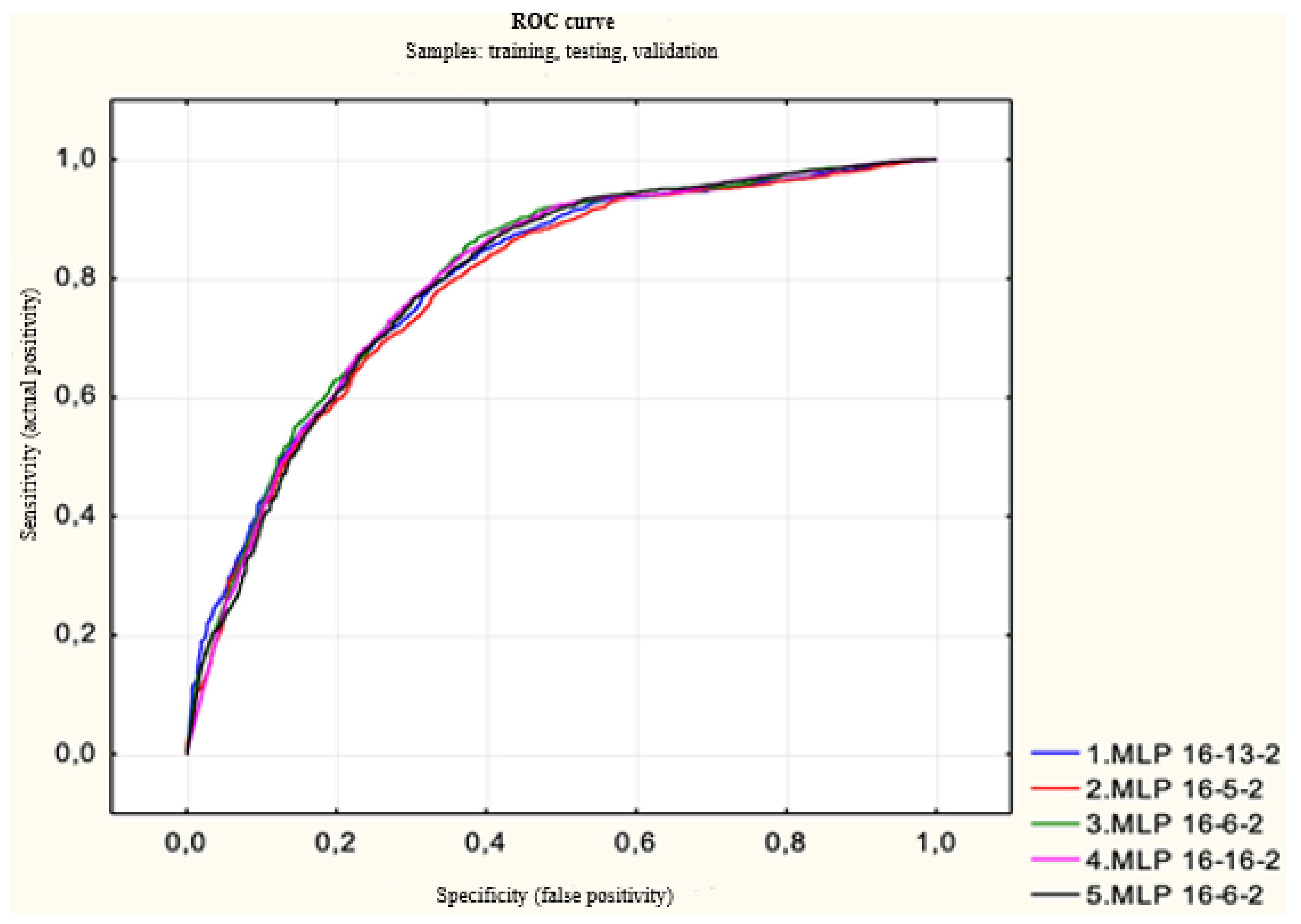
For other possible applications of the model (or of all neural networks), the characteristic of the ROC curve, which evaluates the statistical accuracy of the result, is of interest. For its course, see Figure 2.
The course of the ROC curve is very similar for all the neural networks. The ROC threshold is the point on the curve closest to the coordinate (0, 1) (see Table 7).
The obtained characteristic is then compared with the results obtained using the Mathematica software programme. However, it must be noted that in this case, the ROC is set for the training, testing and validation datasets.

4.2. Mathematica—Neural Networks

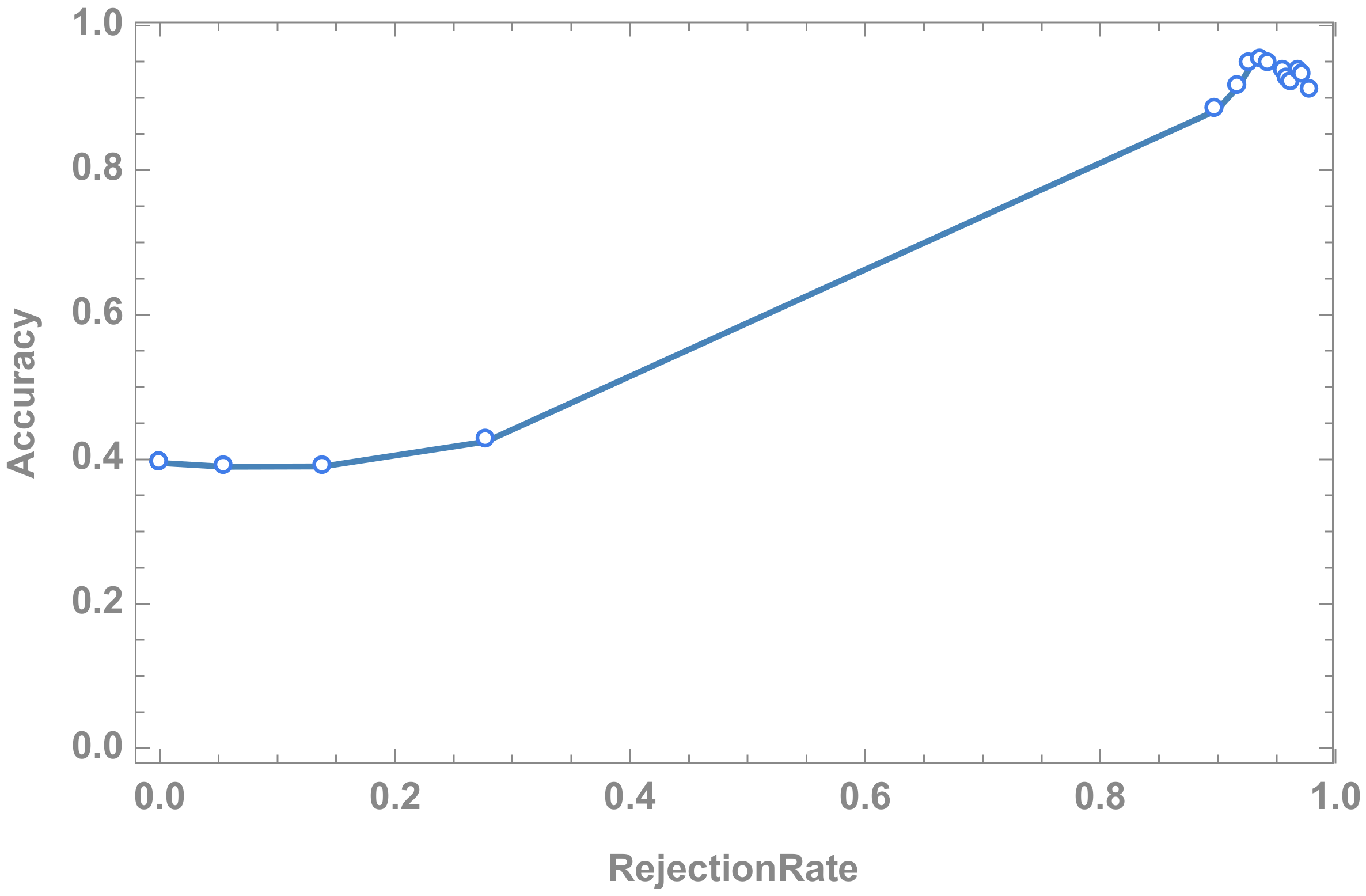
The data for the calculations were divided into training, testing, and validation datasets, as was the case for the Statistica software programme. The results of the calculations using the Mathematica software programme are illustrated in the form of an accuracy-rejection graph (Figure 3).
The calculated average accuracy of the model is 0.745117. This is the average of the baseline precision course shown in Figure 2.
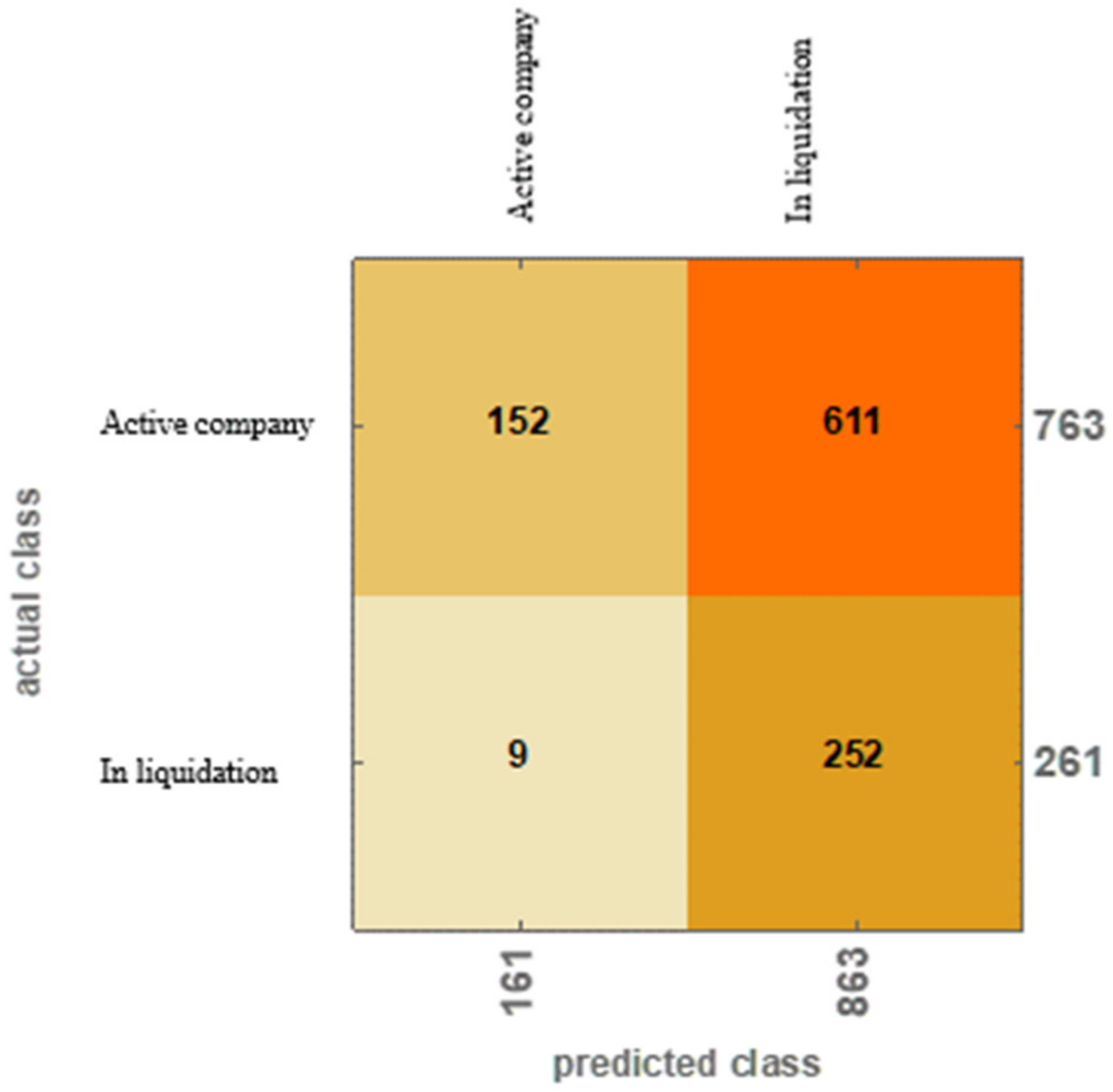
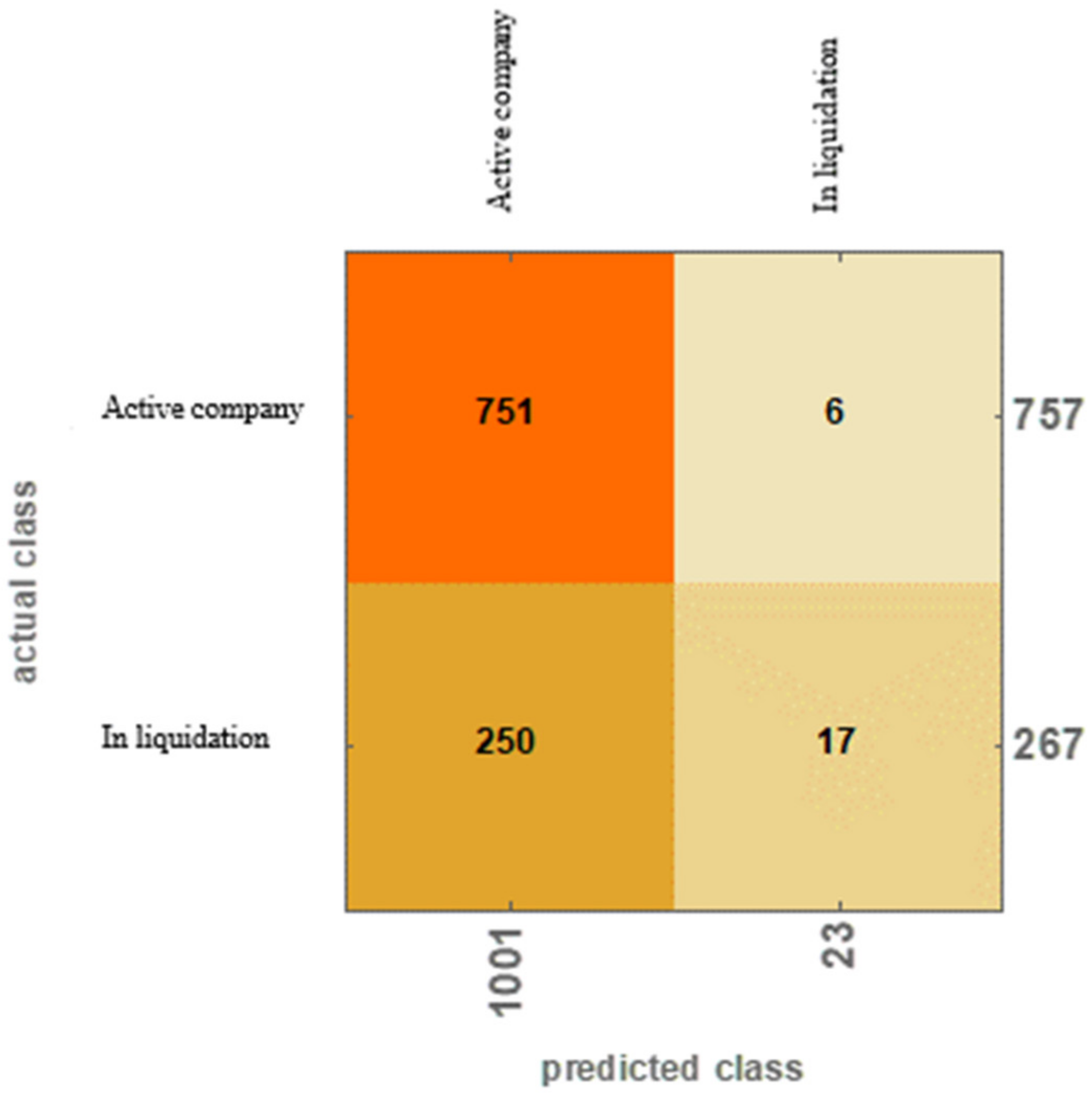
Within the ROC curve, the ROC threshold for the companies capable of surviving potential financial distress and companies in liquidation was determined to be 0.772796. This is expressed in absolute values in the confusion matrix for the testing dataset (see Figure 4). The confusion matrix then confirms the factual accuracy of the results, which proves there is no overfitting.
The matrix indicates that the neural network is able to classify the companies in liquidation well, whereas its capability of classifying those companies able to survive potential financial distress is very low.
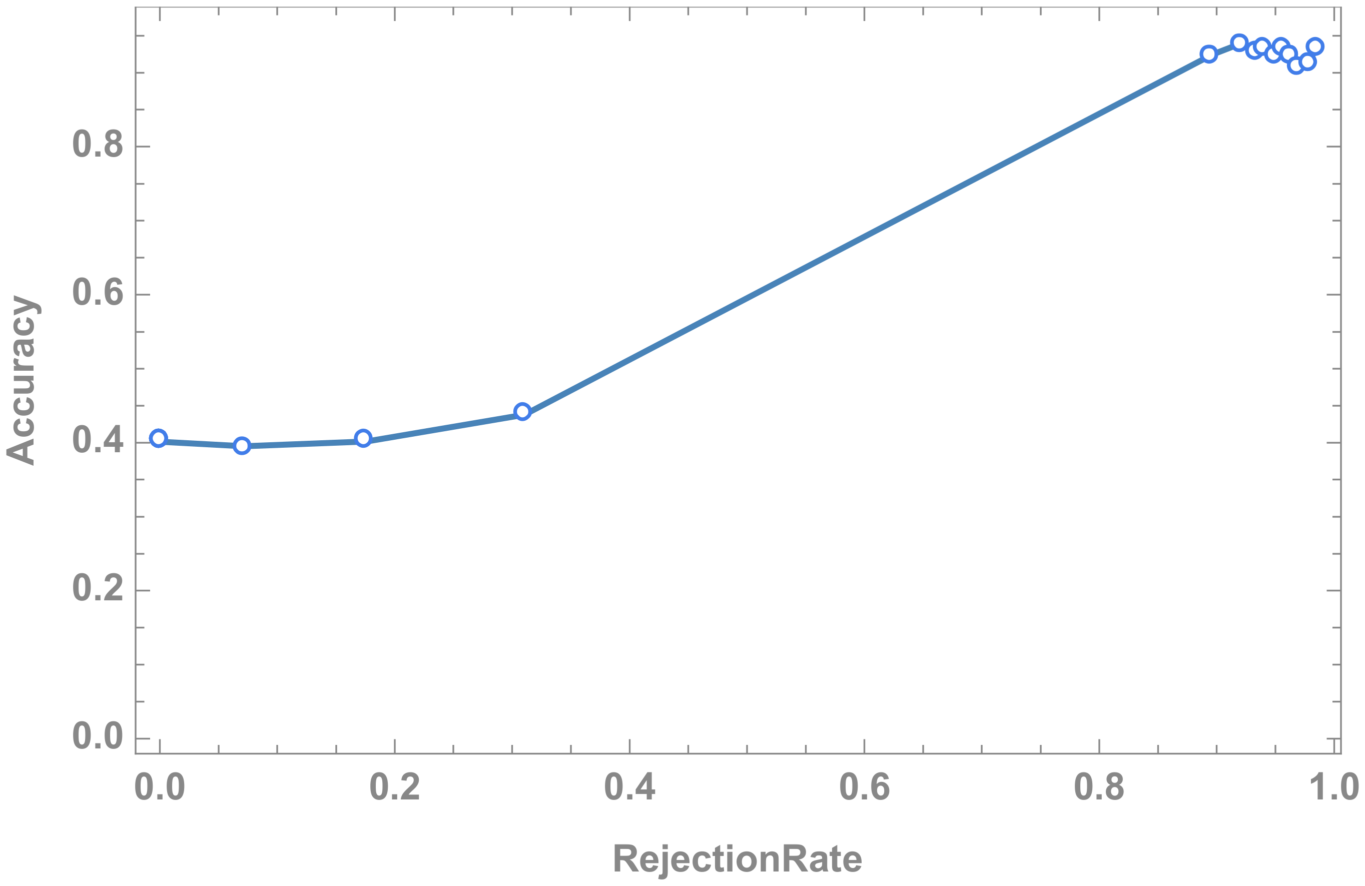
In the case of the validation dataset, the results are slightly different. This is illustrated in the accuracy-rejection graph (Figure 5).
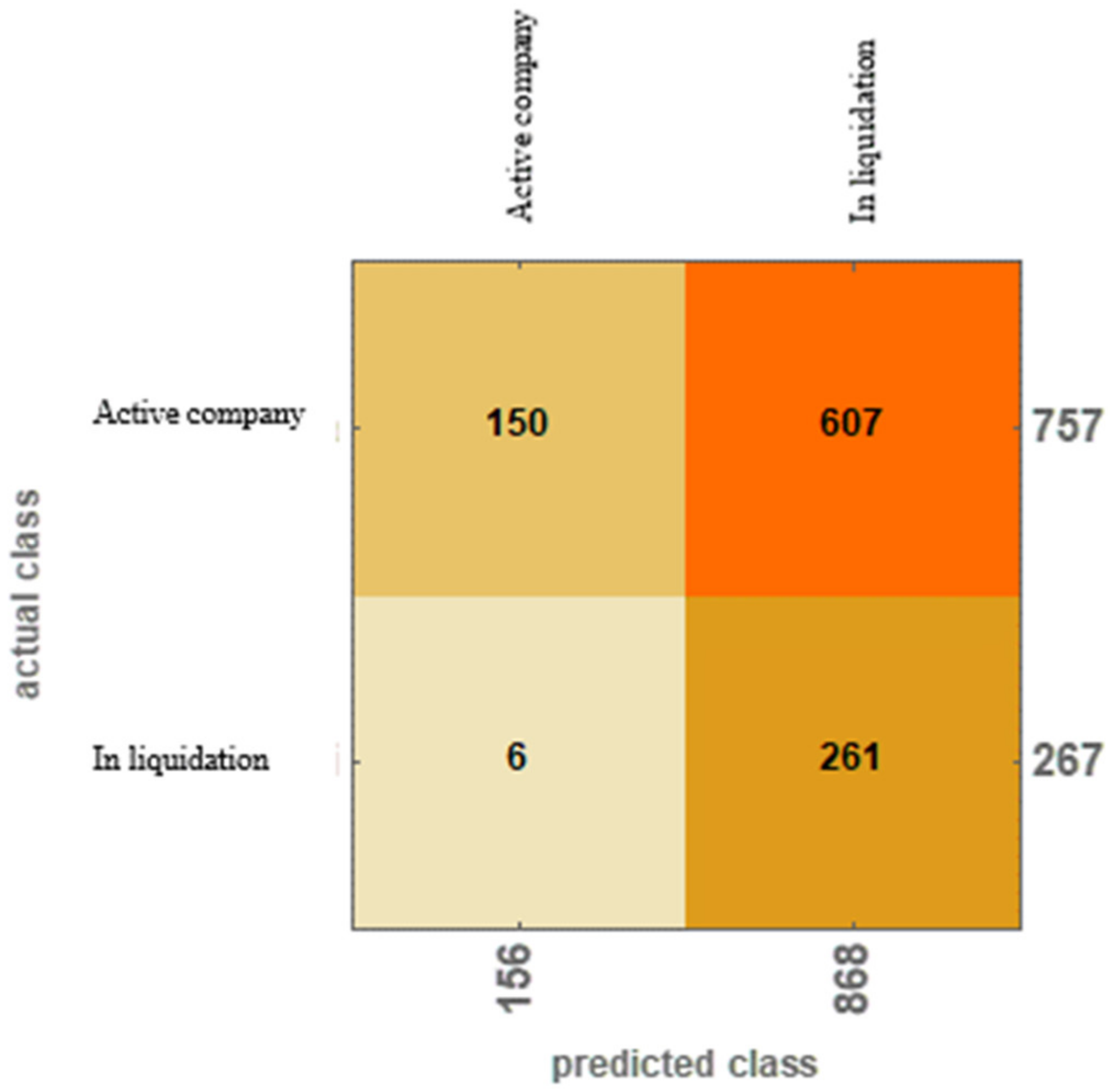
The accuracy of the model for the validation dataset was determined to be 0.739258. The ROC curve threshold for the companies capable of surviving potential financial distress was determined to be 0.77768, and for companies in liquidation 0.776384. This is expressed in the confusion matrix for the validation dataset in absolute values (Figure 6).
The validation dataset verified the applicability of the model, producing approximately the same result as the testing dataset.
The model is applicable for the classification of those companies in liquidation and therefore for the prediction of potential bankruptcy, but not for predicting the survival of a company in the case of potential financial distress.

4.3. Mathematica—Logistic Regression

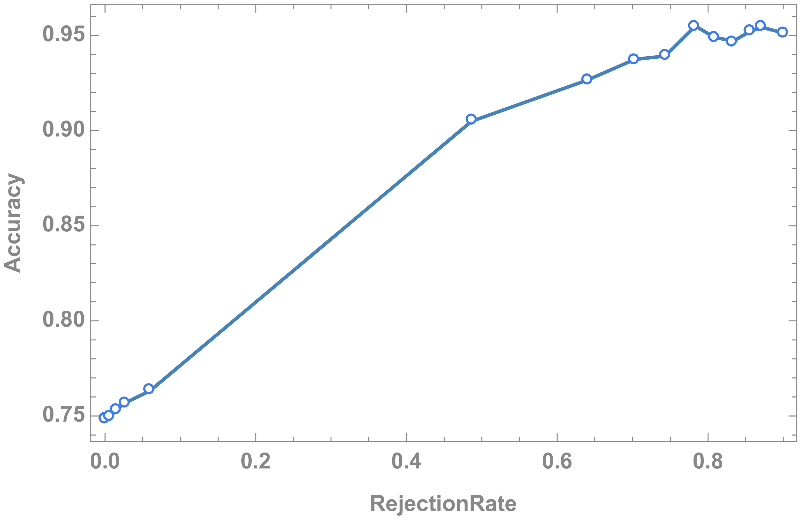
For logistic regression, the dataset was also divided into training, testing, and validation datasets as was the case for the Statistica software programme. Figure 7 shows the accuracy-rejection graph for the testing dataset.
The calculated average accuracy of the model is 0.745117 (The result is the same as in the case of testing dataset result calculated by Mathematica software). This represents the average of the course of the accuracy baseline in Figure 7.
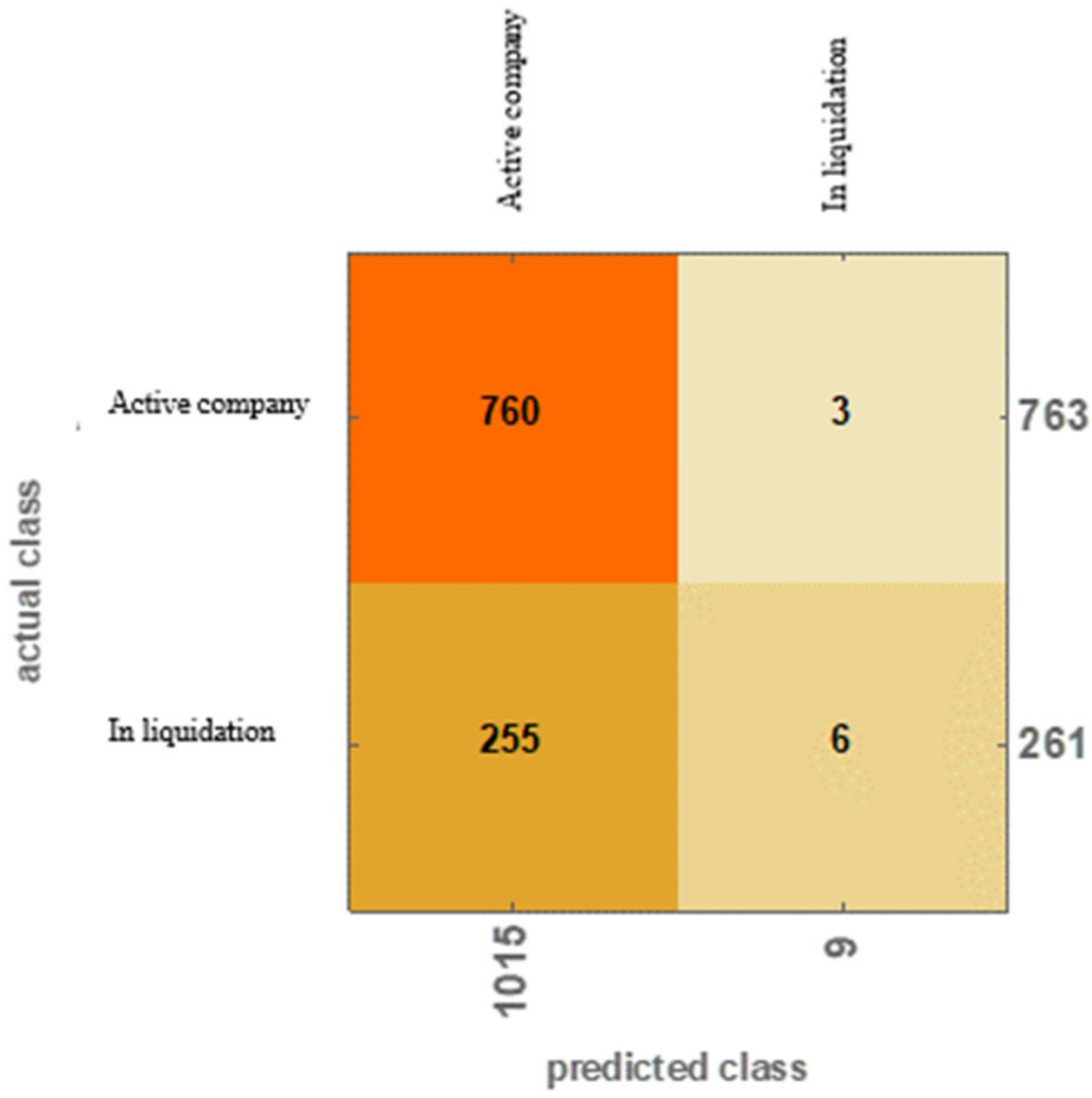
Within the ROC curve, the ROC threshold for the companies capable of surviving potential financial distress was determined to be 0.789458, and for companies in liquidation 0.789478. This is expressed in absolute values in the confusion matrix for the testing dataset (Figure 8).
Even in this case, the model did not produce satisfactory results. It is able to classify active companies with a relatively high level of accuracy, but not those companies in liquidation.
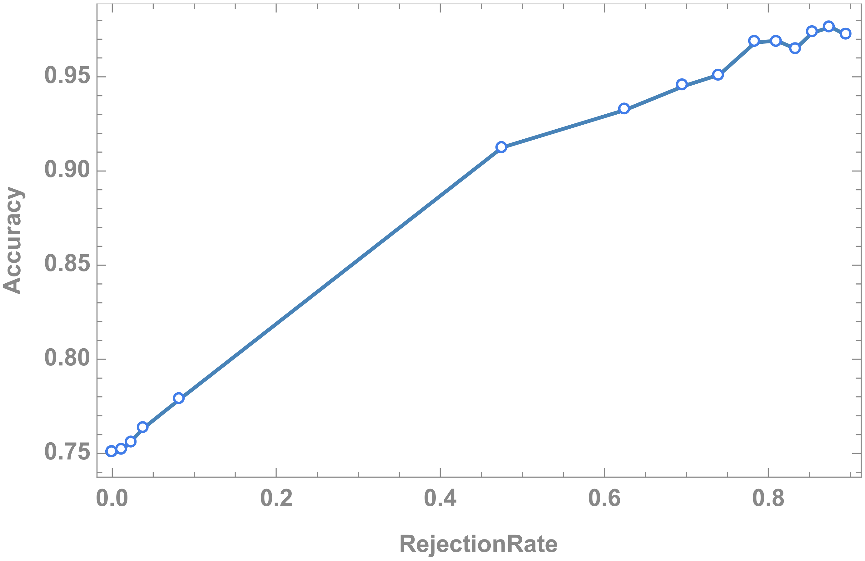
In the case of the validation dataset, the results are slightly different, as illustrated in the following accuracy-rejection graph (Figure 9).
The accuracy of the model for the validation dataset was determined to be 0.739258. The ROC curve threshold for the companies capable of surviving potential financial distress was determined to be 0.831307, and for companies in liquidation 0.831332. This is expressed in absolute values in the confusion matrix for the testing dataset (Figure 10).
The validation and testing datasets produced approximately the same results, thereby verifying the applicability of the model.

5. Discussion

In the Statistica software programme, 10,000 artificial neural networks of the MLP type were generated, of which five with the best parameters were retained. All of them are multilayer perceptron networks. Tsai and Wu [83] claim that a multilayer perceptron (MLP) network trained by a backpropagation algorithm is the most commonly used technique for decision-making concerning financial problems. In all cases during our research, an alternative to the quasi-Newton algorithm was used. For the use of neural networks in the Mathematica software programme, the data for the calculations were divided into training, testing, and validation datasets, as was also the case for the Statistica software programme. The results of the calculations obtained from the Mathematica software programme were illustrated in the form of an accuracy-rejection graph. The validation and testing datasets produced approximately the same results, thereby verifying the applicability of the model. This model, created in the Mathematica software programme, can be used to classify companies in liquidation and therefore to predict possible bankruptcy, but not to predict a company’s survival in the event of potential financial distress. The results show that the models created using the Mathematica software programme are not applicable in practice due to the parameters of the obtained results. The results are not satisfactory. On the other hand, the artificial neural structures obtained using the neural network model in Statistica are prospective due to their performance, which is almost always above 0.8, and the logical economic interpretation of the relevant variables. All the generated and maintained networks show excellent performance, with few errors. The excellent performance of neural networks and their application to bankruptcy prediction is also confirmed by Wilson and Sharda [84], who compared the predictive accuracy of BPNN with the accuracy of DA (discriminant analysis). They used Altman variables and concluded that BPNN outperformed other methods in all the samples tested. Boritz and Kennedy [85], who tested the performance of artificial neural networks for bankruptcy prediction against discriminant analysis and logit and probit, show that the performance of the tested neural networks is sensitive to the selected variables and that networks cannot be relied upon to “transform” variables and focus on the most important variables (network performance based on a combined set of Ohlson and Altman data was often worse than for one of the subsets). It is also important to note that the results are very sensitive to sampling error. Angellini, Tollo, and Roli [86] describe a case in which neural networks are successfully applied to credit risk assessment. They also developed two neural network systems, one with a standard forward network and the other with a special architecture. The application was tested on real data related to small Italian businesses. It has been shown that neural networks can be very successful in learning and estimating a debtor’s default tendency, provided that careful data analysis, pre-processing, and training are performed. Zhang et al. [87] compared neural networks with logistic regression, a known statistical classification method. According to them, neural networks provide a significantly better estimate of the classification rate for the unknown population, as well as for the invisible part of the population. It is easy to say that the cost of not predicting bankruptcy is much higher than the cost of a bankrupt company. The neural networks in the study clearly show their superiority over logistic regression in the prediction of company bankruptcy. Even in the case of our research, neural networks have proven to be a suitable tool for problems related to the prediction of company bankruptcy, thereby specifying the software that is most suitable for data processing and which produces the best results. A similar result was achieved by Horák, Vrbka, and Šuleř [80], whose aim was to create a model for predicting the potential bankruptcy of companies using appropriate classification methods, especially Support Vector Machine and artificial neural networks, and to evaluate the results of those methods. They came to the conclusion that the most successful model applicable in practice is the model determined by the neural structure 2.MLP 22-9-2. The Support Vector Machine model showed a relatively high level of accuracy, but was not usable in the structure of correct classifications.

6. Conclusions

The objective of this contribution was to develop a comprehensive method for the evaluation of an industrial company that could be used for predicting possible bankruptcy in the future.
Three tools were used for the development of the method. First, data were selected and processed by means of a scientific experiment. Then the tools and various system settings were tested. Subsequently, the results were verified on two individual datasets—testing and validation. The results show that the ratio of companies was correct and that the neural networks did not miss companies in liquidation either. We verified that there was no overfitting and so we were able to publish the article. ROC and confusion matrices are perfectly sufficient for evaluating success. The ROC evaluates the statistically correct result. The confusion matrix then confirms the factual accuracy of the results. Other methods should then duplicate the two. Although it was possible to use other methods, the benefit of duplicate validation is zero because they show the same as ROC and confusion matrices. From the point of view of this contribution, this would mean confirmation of the confirmed and the artificial extension of this contribution. The results show that the models created by means of the Mathematica software programme are not applicable in practice due to the parameters of the results obtained. The results are not satisfactory. On the other hand, the artificial neural structures obtained by means of the model of neural networks using the Statistica software programme are prospective due to their performance, which is almost always above 0.8, and the logical economic interpretation of the variables involved. All the generated and retained networks show excellent performance, with few errors. However, one of the artificial structures, network no. 4 (MLP 16-16-2), produces better results than the others. Overall accuracy is almost 81%, the classification of companies capable of surviving financial distress is almost 90%, and the classification of companies at risk of bankruptcy almost is 55%. It therefore meets the essential prerequisite for application in practice, namely the result of the prediction is not accidental with a probability of 50%. The advantage of neural structures and the application of the methodology outlined in this contribution is, to a certain extent, the adaptability of the model to a specific group of companies. In this case, it concerned industrial companies in the Czech Republic. It should also be noted that the model was generated based on past data for a certain period and that it is necessary to train the network again for a certain period so that it still generates satisfactory results. The shorter this interval is, the more accurate the results will become over time.
Often, organizations limit their management to financial information. However, in the last few years, so-called sustainable performance has been promoted, which, as already outlined, not only highlights economic aspects, but also the equal importance of environmental and social aspects. If we therefore want to ensure greater sustainability for the next generation and maintain the position of a business entity on the market, it is necessary to include non-financial indicators in the performance measurement system as well.
For this reason, the future line of research will focus on the direct incorporation of other non-financial factors, such as environmental and social performance indicators, into the model for the comprehensive evaluation of a company and the prediction of possible bankruptcy.

Author Contributions

Conceptualization, J.H. and T.K.; methodology, J.H., Z.R., and T.K.; software, J.H. and Z.R.; validation, Z.R. and V.M.; formal analysis, V.M.; investigation, Z.R.; resources, T.K. and V.M.; data curation, Z.R., J.H., and T.K.; writing—original draft preparation, J.H., Z.R., and T.K.; writing—review and editing, V.M.; visualization, V.M.; supervision, Z.R.; project administration, J.H. All authors have read and agreed to the published version of the manuscript.

Funding

This research received no external funding.

Conflicts of Interest

The authors declare no conflict of interest.

References

  1. Laaksonen, O.; Peltoniemi, M. The essence of dynamic capabilities and their measurement. Int. J. Manag. Rev. 2018, 20, 184–205. [Google Scholar] [CrossRef]
  2. Bohanec, M.; Kljajić Borštnar, M.; Robnik-Šikonja, M. Explaining machine learning models in sales predictions. Expert Syst. Appl. 2017, 71, 416–428. [Google Scholar] [CrossRef]
  3. Melo, L., Jr.; Nardini, F.M.; Renso, C.; Trani, R.; Macedo, J.A. A novel approach to define the local region of dynamic selection techniques in imbalanced credit scoring problems. Expert Syst. Appl. 2020, 152. [Google Scholar] [CrossRef]
  4. Klieštik, T.; Valášková, K.; Lazaroiu, G.; Kováčová, M.; Vrbka, J. Remaining financially healthy and competitive: The role of financial predictors. J. Compet. 2020, 12, 74–92. [Google Scholar] [CrossRef]
  5. Devi, S.S.; Radhika, Y. A survey on machine learning and statistical techniques in bankruptcy prediction. Int. J. Mach. Learn. Comput. 2018, 8. [Google Scholar] [CrossRef] [Green Version]
  6. Liu, J.; Wu, C. Company financial path analysis using Fuzzy C-means and its application in financial failure prediction. J. Bus. Econ. Manag. 2018, 19, 213–234. [Google Scholar] [CrossRef] [Green Version]
  7. Loprevite, S.; Raucci, D.; Rupo, D. Reporting KPIs and financial performance in the transition to mandatory disclosure: The case of Italy. Sustainability 2020, 12, 5195. [Google Scholar] [CrossRef]
  8. Da Costa, S.F.; Boente, D.R. Evaluation of financial performance of corporate sustainability index companies through data envelopment analysis. Rev. Ambiente Contab. 2011, 3, 75–99. [Google Scholar]
  9. Grandhi, S.; Wibowo, S. Sustainability performance evaluation of automotive manufacturing companies. In Proceedings of the 2016 IEEE 11th Conference on Industrial Electronics and Applications (ICIEA), Hefei, China, 5–7 June 2016; IEEE: New York, NY, USA, 2016; pp. 1725–1730. [Google Scholar]
  10. Hawrysz, L.; Maj, J. Identification of stakeholders of public interest organisations. Sustainability 2017, 9, 1609. [Google Scholar] [CrossRef] [Green Version]
  11. Lombardo, G.; Mazzocchetti, A.; Rapallo, I.; Tayser, N.; Cincotti, S. Assessment of the economic and social impact using SROI: An application to sport companies. Sustainability 2019, 11, 3612. [Google Scholar] [CrossRef] [Green Version]
  12. Hardinata, L.; Warsito, B. Bankruptcy prediction based on financial ratios using Jordan Recurrent Neural Networks: A case study in Polish companies. J. Phys. Conf. Ser. 2018, 1025, 012098. [Google Scholar] [CrossRef]
  13. Messai, A.S.; Gallali, M.I. Financial leading indicators of banking distress: A micro prudential approach-evidence from Europe. Asian Soc. Sci. 2015, 11, 78–90. [Google Scholar] [CrossRef] [Green Version]
  14. Chen, M.Y. Bankruptcy prediction in firms with statistical and intelligent techniques and a comparison of evolutionary computation approaches. Comput. Math. Appl. 2011, 62, 4514–4524. [Google Scholar] [CrossRef] [Green Version]
  15. Abdou, H.; Abd Allah, W.; Mulkeen, J.; Ntim, C.G.; Wang, Y. Prediction of financial strength ratings using machine learning and conventional techniques. Investig. Manag. Financ. Innov. 2017, 14, 194–211. [Google Scholar] [CrossRef] [Green Version]
  16. Vochozka, M. Formation of complex company evaluation method through neural networks based on the example of construction companies’ collection. AD ALTA J. Interdiscip. Res. 2017, 7, 232–239. [Google Scholar]
  17. Vochozka, M.; Vrbka, J. Estimation of the development of the Euro to Chinese Yuan exchange rate using artificial neural networks. In Proceedings of the SHS Web of Conferences: Innovative Economic Symposium 2018—Milestones and Trends of World Economy (IES2018), Beijing, China, 8–9 November 2018; Horak, J., Ed.; EDP Sciences: Les Ulis, France, 2019. [Google Scholar] [CrossRef]
  18. Kovacova, M.; Kliestikova, J. Modelling bankruptcy prediction models in Slovak companies. In Proceedings of the SHS Web of Conferences: Innovative Economic Symposium 2017—Strategic Partnership in International Trade, Ceske Budejovice, Czech Republic, 19 October 2017; Vachal, J., Vochozka, M., Horak, J., Eds.; EDP Sciences: Les Ulis, France, 2017; p. 39. [Google Scholar] [CrossRef] [Green Version]
  19. Sayari, N.; Mugan, C.S. Industry specific financial distress modeling. BRQ Bus. Res. Q. 2017, 20, 45–62. [Google Scholar] [CrossRef] [Green Version]
  20. Chen, H.L. Development of a stable corporate bankruptcy classification model: Evidence from Taiwan. Int. J. Econ. Sci. 2018, 7, 16–38. [Google Scholar] [CrossRef]
  21. Alaminos, D.; Castillo, A.; Fernández, M.Á. A global model for bankruptcy prediction. PLoS ONE 2016, 11. [Google Scholar] [CrossRef] [Green Version]
  22. Hu, H.; Sathye, M. Predicting financial distress in the Hong Kong growth enterprises market from the perspective of financial sustainability. Sustainability 2015, 7, 1186–1200. [Google Scholar] [CrossRef] [Green Version]
  23. Vochozka, M. Development of methods for comprehensive evaluation of business performance. Politická Ekon. 2010, 2010, 675–688. [Google Scholar] [CrossRef] [Green Version]
  24. Salinas, D.; Flunkert, V.; Gasthaus, J.; Januschowski, T. DeepAR: Probabilistic forecasting with autoregressive recurrent networks. Int. J. Forecast. 2020, 36, 1181–1191. [Google Scholar] [CrossRef]
  25. Lei, Z. Research and analysis of deep learning algorithms for investment decision support model in electronic commerce. Electron. Commer. Res. 2020, 20, 275–295. [Google Scholar] [CrossRef]
  26. Khashei, M.; Hajirahimi, Z. Performance evaluation of series and parallel strategies for financial time series forecasting. Financ. Innov. 2017, 3. [Google Scholar] [CrossRef] [Green Version]
  27. Kolupaieva, I.; Pustovhar, S.; Suprun, O.; Shevchenko, O. Diagnostics of systemic risk impact on the enterprise capacity for financial risk neutralization: The case of Ukrainian metallurgical enterprises. Oeconomia Copernic. 2019, 10, 471–491. [Google Scholar] [CrossRef] [Green Version]
  28. Lohmann, C.; Ohliger, T. The total cost of misclassification in credit scoring: A comparison of generalized linear models and generalized additive models. J. Forecast. 2019, 38, 375–389. [Google Scholar] [CrossRef]
  29. Gulsoy, N.; Kulluk, S. A data mining application in credit scoring processes of small and medium enterprises commercial corporate customers. Wiley Interdiscip. Rev. Data Min. Knowl. Discov. 2018, 9. [Google Scholar] [CrossRef]
  30. Atsalakis, G.S. Using computational intelligence to forecast carbon prices. Appl. Soft Comput. 2016, 43, 107–116. [Google Scholar] [CrossRef]
  31. Šestanović, T.; Arnerić, J. Neural network structure identification in inflation forecasting. J. Forecast. 2020. [Google Scholar] [CrossRef]
  32. Wang, Z.; Zhang, J.; Ji, S.; Meng, C.; Li, T.; Zheng, Y. Predicting and ranking box office revenue of movies based on big data. Inf. Fusion 2020, 60, 25–40. [Google Scholar] [CrossRef]
  33. Huber, J.; Müller, S.; Fleischmann, M.; Stuckenschmidt, H. A data-driven newsvendor problem: From data to decision. Eur. J. Oper. Res. 2019, 278, 904–915. [Google Scholar] [CrossRef]
  34. Cao, J.; Wang, J. Exploration of stock index change prediction model based on the combination of principal component analysis and artificial neural network. Soft Comput. 2020, 24, 7851–7860. [Google Scholar] [CrossRef]
  35. Kim, E.; Lee, J.; Shin, H. Champion-challenger analysis for credit card fraud detection: Hybrid ensemble and deep learning. Expert Syst. Appl. 2019, 128, 214–224. [Google Scholar] [CrossRef]
  36. Kim, J.; Kim, H.J.; Kim, H. Fraud detection for job placement using hierarchical clusters-based deep neural networks. Appl. Intell. 2019, 49, 2842–2861. [Google Scholar] [CrossRef]
  37. Loureiro, A.L.D.; Miguéis, V.L.; Da Silva, L.F.M. Exploring the use of deep neural networks for sales forecasting in fashion retail. Decis. Support Syst. 2018, 114, 81–93. [Google Scholar] [CrossRef]
  38. Wei, C.C.; Cheng, Y.L. Six Sigma project selection using fuzzy multiple attribute decision-making method. Total Qual. Manag. Bus. Excell. 2020, 31, 1266–1289. [Google Scholar] [CrossRef]
  39. Mahdiraji, H.A.; Zavadskas, E.Z.; Skare, M.; Kafshgar, F.Z.R.; Arab, A. Evaluating strategies for implementing industry 4.0: A hybrid expert-oriented approach of BWM and interval valued intuitionistic fuzzy TODIM. Econ. Res. Ekon. Istraživanja 2020, 33, 1600–1620. [Google Scholar] [CrossRef]
  40. Li, Z.X.; Liu, J.Y.; Luo, D.K.; Wang, J.J. Study of evaluation method for the overseas oil and gas investment based on risk compensation. Pet. Sci. 2020, 17, 858–871. [Google Scholar] [CrossRef]
  41. Wang, Y.; Jin, X. Structural risk of diversified project financing of city investment company in China based on the best worst method. Eng. Constr. Archit. Manag. 2019. [Google Scholar] [CrossRef]
  42. De, G.; Tan, Z.; Li, M.; Huang, L.; Wang, Q.; Li, H. A credit risk evaluation based on intuitionistic fuzzy set theory for the sustainable development of electricity retailing companies in China. Energy Sci. Eng. 2019, 7, 2825–2841. [Google Scholar] [CrossRef]
  43. Wang, L.; Chen, Y.; Jiang, H.; Yao, J. Imbalanced credit risk evaluation based on multiple sampling, multiple kernel fuzzy self-organizing map and local accuracy ensemble. Appl. Soft Comput. 2020, 91. [Google Scholar] [CrossRef]
  44. Wu, Y.; Zhou, J. Risk assessment of urban rooftop distributed PV in energy performance contracting (EPC) projects: An extended HFLTS-DEMATEL fuzzy synthetic evaluation analysis. Sustain. Cities Soc. 2019, 47. [Google Scholar] [CrossRef]
  45. Liang, K.; He, J. Analyzing credit risk among Chinese P2P-lending businesses by integrating text-related soft information. Electron. Commer. Res. Appl. 2020, 40. [Google Scholar] [CrossRef]
  46. Li, Y.; Chen, W. Entropy method of constructing a combined model for improving loan default prediction: A case study in China. J. Oper. Res. Soc. 2019, 1–11. [Google Scholar] [CrossRef]
  47. Murè, S.; Comberti, L.; Demichela, M. How harsh work environments affect the occupational accident phenomenology? Risk assessment and decision making optimisation. Saf. Sci. 2017, 95, 159–170. [Google Scholar] [CrossRef]
  48. Zhao, J.; Fan, W.; Zhai, X. Identification of land-use characteristics using bicycle sharing data: A deep learning approach. J. Transp. Geogr. 2020, 82. [Google Scholar] [CrossRef]
  49. Sajnóg, A.R. Executive compensation and comprehensive income: Evidence from Polish listed companies. Oeconomia Copernic. 2019, 10, 493–509. [Google Scholar] [CrossRef]
  50. Lee, J.M.; Jeong, Y.K.; Woo, J.H. Development of an evaluation framework of production planning for the shipbuilding industry. Int. J. Comput. Integr. Manuf. 2018, 31, 831–847. [Google Scholar] [CrossRef]
  51. Hanine, M.; Boutkhoum, O.; Agouti, T.; Tikniouine, A. A new integrated methodology using modified Delphi-fuzzy AHP-PROMETHEE for geospatial business intelligence selection. Inf. Syst. E Bus. Manag. 2017, 15, 897–925. [Google Scholar] [CrossRef]
  52. Borges, L.A.; Tan, K.H. Incorporating human factors into the AAMT selection: A framework and process. Int. J. Prod. Res. 2016, 55, 1459–1470. [Google Scholar] [CrossRef]
  53. Ban, A.I.; Ban, O.I.; Bogdan, V.; Sabau Popa, D.C.; Tuse, D. Performance evaluation model of Romanian manufacturing listed companies by Fuzzy AHP and TOPSIS. Technol. Econ. Dev. Econ. 2020, 26, 808–836. [Google Scholar] [CrossRef]
  54. Yang, L.W.; Aggarwal, P.; Peracchio, L.; Johar, G.; Campbell, M.C. No small matter: How company size affects consumer expectations and evaluations. J. Consum. Res. 2019, 45, 1369–1384. [Google Scholar] [CrossRef]
  55. Kuo, K.C.; Kweh, Q.L.; Ting, I.W.K.; Azizan, N.A. Dynamic network performance evaluation of general insurance companies: An insight into risk management committee structure. Total Qual. Manag. Bus. Excell. 2015, 28, 542–558. [Google Scholar] [CrossRef]
  56. Hsu, Y.F.; Lee, W.P. Evaluation of the going-concern status for companies: An ensemble framework-based model. J. Forecast. 2020, 39, 687–706. [Google Scholar] [CrossRef]
  57. Petropoulos, A.; Siakoulis, V.; Stavroulakis, E.; Vlachogiannakis, N.E. Predicting bank insolvencies using machine learning techniques. Int. J. Forecast. 2020, 36, 1092–1113. [Google Scholar] [CrossRef]
  58. Ye, X.; Dong, L.; Ma, D. Loan evaluation in P2P lending based on Random Forest optimized by genetic algorithm with profit score. Electron. Commer. Res. Appl. 2018, 32, 23–36. [Google Scholar] [CrossRef]
  59. Salminen, J.; Yoganathan, V.; Corporan, J.; Jansen, B.J.; Jung, S.G. Machine learning approach to auto-tagging online content for content marketing efficiency: A comparative analysis between methods and content type. J. Bus. Res. 2019, 101, 203–217. [Google Scholar] [CrossRef]
  60. Qiao, W.; Yang, Z.; Kang, Z.; Pan, Z. Short-term natural gas consumption prediction based on Volterra adaptive filter and improved whale optimization algorithm. Eng. Appl. Artif. Intell. 2020, 87. [Google Scholar] [CrossRef]
  61. Ojstersek, R.; Buchmeister, B. The impact of manufacturing flexibility and multi-criteria optimization on the sustainability of manufacturing systems. Symmetry 2020, 12, 157. [Google Scholar] [CrossRef] [Green Version]
  62. Li, J.; Wu, F.; Li, J.; Zhao, Y. Research on risk evaluation of transnational power networking projects based on the Matter-element extension theory and granular computing. Energies 2017, 10, 1523. [Google Scholar] [CrossRef]
  63. Makridakis, S.; Spiliotis, E.; Assimakopoulos, V. The M4 Competition: 100,000 time series and 61 forecasting methods. Int. J. Forecast. 2020, 36, 54–74. [Google Scholar] [CrossRef]
  64. Gao, Y.; Fan, Y.; Wang, J.; Duan, Z. Evaluation of governmental safety regulatory functions in preventing major accidents in China. Saf. Sci. 2019, 120, 299–311. [Google Scholar] [CrossRef]
  65. Han, S.; Cao, B.; Fu, Y.; Luo, Z. A liner shipping competitive model with consideration of service quality management. Ann. Oper. Res. 2018, 270, 155–177. [Google Scholar] [CrossRef]
  66. Yazdani, M.; Pamucar, D.; Chatterjee, P.; Chakraborty, S. Development of a decision support framework for sustainable freight transport system evaluation using rough numbers. Int. J. Prod. Res. 2020, 58, 4325–4351. [Google Scholar] [CrossRef]
  67. Wang, R.; Li, Y. A novel approach for green supplier selection under a q-Rung orthopair fuzzy environment. Symmetry 2018, 10, 687. [Google Scholar] [CrossRef] [Green Version]
  68. Luo, X.; Wang, Z.; Lu, L.; Guan, Y. Supply chain flexibility evaluation based on matter-element extension. Complexity 2020, 2020, 8057924. [Google Scholar] [CrossRef]
  69. Castro, N.R.; Chousa, P.J. An integrated framework for the financial analysis of sustainability. Bus. Strategy Environ. 2006, 15, 322–333. [Google Scholar] [CrossRef]
  70. Maciková, L.; Smorada, M.; Dorčák, P.; Beug, B.; Markovič, P. Financial aspects of sustainability: An evidence from Slovak companies. Sustainability 2018, 10, 2274. [Google Scholar] [CrossRef] [Green Version]
  71. Rita, D.I.G.; Fernando, A.F.; Meidute-Kavaliauskiene, L. Proposal of a green index for small and medium-sized enterprises: A multiple criteria group decision-making approach. J. Clean. Prod. 2018, 196, 985–996. [Google Scholar] [CrossRef]
  72. Escrig-Olmedo, E.; Muñoz-Torres, M.J.; Fernández-Izquierdo, M.Á.; Rivera-Lirio, J.M. Measuring corporate environmental performance: A methodology for sustainable development. Bus. Strategy Environ. 2017, 26, 142–162. [Google Scholar] [CrossRef]
  73. Fatma, M.; Khan, I. An investigation of consumer evaluation of authenticity of their company’s CSR engagement. Total Qual. Manag. Bus. Excell. 2020, 1–18. [Google Scholar] [CrossRef]
  74. Schaefer, S.D.; Terlutter, R.; Diehl, S. Is my company really doing good? Factors influencing employees’ evaluation of the authenticity of their company’s corporate social responsibility engagement. J. Bus. Res. 2019, 101, 128–143. [Google Scholar] [CrossRef]
  75. Vrbka, J.; Nica, E.; Podhorská, I. The application of Kohonen networks for identification of leaders in the trade sector in Czechia. Equilib. Q. J. Econ. Econ. Policy 2019, 14, 739–761. [Google Scholar] [CrossRef]
  76. Král, P.; Musa, H.; Lazaroiu, G.; Mišanková, M.; Vrbka, J. Comprehensive assessment of the selected indicators of financial analysis in the context of failing companies. J. Int. Stud. 2018, 11, 282–294. [Google Scholar] [CrossRef]
  77. Vochozka, M.; Vrbka, J.; Suler, P. Bankruptcy or success? The effective prediction of a company’s financial development using LSTM. Sustainability 2020, 12, 7529. [Google Scholar] [CrossRef]
  78. Machová, V.; Vochozka, M. Analysis of business companies based on artificial neural networks. In Proceedings of the SHS Web of Conferences: Innovative Economic Symposium 2018—Milestones and Trends of World Economy (IES2018), Beijing, China, 8–9 November 2018; Horak, J., Ed.; EDP Sciences: Les Ulis, France, 2019. [Google Scholar] [CrossRef]
  79. Vrbka, J. The use of neural networks to determine value based drivers for SMEs operating in the rural areas of the Czech Republic. Oeconomia Copernic. 2020, 11, 325–346. [Google Scholar] [CrossRef]
  80. Horák, J.; Vrbka, J.; Šuleř, P. Support vector machine methods and artificial neural networks used for the development of bankruptcy prediction models and their comparison. J. Risk Financ. Manag. 2020, 13, 60. [Google Scholar] [CrossRef] [Green Version]
  81. Khasaev, G.; Vochozka, M.; Vrbka, J. Creating a Comprehensive Enterprise Evaluation Method, 1st ed.; Institute of Technology and Business: Ceske Budejovice, Czech Republic, 2018. [Google Scholar]
  82. Wöhe, G.; Kislingerová, E. Úvod do Podnikového Hospodářství, 2nd ed.; Beck: Prague, Czech Republic, 2007. [Google Scholar]
  83. Tsai, C.H.F.; Wu, J.W. Using neural network ensembles for bankruptcy prediction and credit scoring. Expert Syst. Appl. 2008, 34, 2639–2649. [Google Scholar] [CrossRef]
  84. Wilson, R.L.; Sharda, R. Bankruptcy prediction using neural networks. Decis. Support Syst. 1994, 11, 545–557. [Google Scholar] [CrossRef]
  85. Boritz, J.E.; Kennedy, D.B. Effectiveness of neural network types for prediction of business failure. Expert Syst. Appl. 1995, 9, 503–512. [Google Scholar] [CrossRef]
  86. Angelini, E.; Tollo, G.; Roli, A. A neural network approach for credit risk evaluation. Q. Rev. Econ. Financ. 2008, 48, 733–755. [Google Scholar] [CrossRef]
  87. Zhang, G.; Hu, M.Y.; Patuwo, B.E.; Indro, D.C. Artificial neural networks in bankruptcy prediction: General framework and cross-validation analysis. Eur. J. Oper. Res. 1999, 116, 16–32. [Google Scholar] [CrossRef] [Green Version]
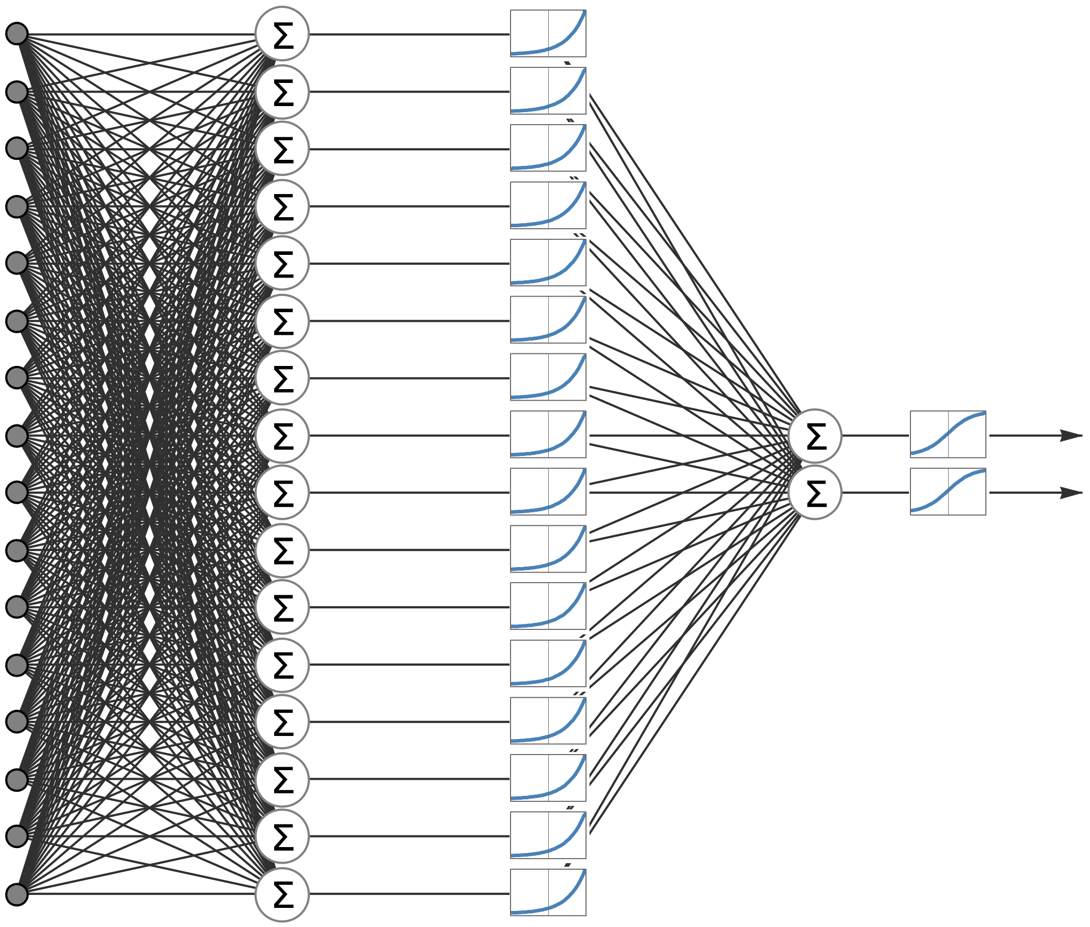
Figure 1. Diagram of 4th retained artificial neural network—MLP 16-16-2.
Sustainability 12 09114 g001
Figure 2. Course of receiver operating characteristic (ROC) curves for retained neural networks.
Sustainability 12 09114 g002
Figure 3. Accuracy-rejection graph for the testing dataset.
Sustainability 12 09114 g003
Figure 4. Confusion matrix for the testing dataset.
Sustainability 12 09114 g004
Figure 5. Accuracy-rejection graph for the validation dataset.
Sustainability 12 09114 g005
Figure 6. Confusion matrix for the validation dataset.
Sustainability 12 09114 g006
Figure 7. Accuracy-rejection graph for the testing dataset.
Sustainability 12 09114 g007
Figure 8. Confusion matrix for the testing dataset.
Sustainability 12 09114 g008
Figure 9. Accuracy-rejection graph for the validation dataset.
Sustainability 12 09114 g009
Figure 10. Confusion matrix for the validation dataset.
Sustainability 12 09114 g010
Table 1. Basic statistical characteristics of the dataset.
SamplesMinimumMaximumAverageStandard Deviation
AKTIVACELK −200162,924,68489,2981,037,658
OBEZNAA −151932,066,56248,783559,746
STALAA−19,06530,832,57639,870495,025
Z−3734,164,87513,496103,764
KP −186827,683,66826,142424,387
FM −23,3764,610,658719380,064
VLASTNIJM −20,871,61153,318,74443,077773,114
HVML −18,657,83639,090,53111,005535,924
HVUO −5,031,6817,010,0194806127,604
CIZIZDROJE −858727,125,36445,364520,891
KZ −858726,176,36728,057369,745
TZPZ −113,372,651911278,647
TZPVVAS −119392,212,22796,9061,308,452
PRIDHODN −2,160,47313,303,71323,397208,063
MZDN 01,920,798901743,568
OHANIM −13,8392,146,145383836,008
Table 2. Basic statistical characteristics of the individual datasets.
SamplesMin. (Train.)Max. (Train.)Average
(Train.)
Standard Deviation (Train.)Min. (Test.)Max. (Test.)Average (Test.)Standard Deviation (Test.)Min. (Valid.)Max. (Valid.)Average (Valid.)Standard Deviation (Valid.)
AKTIVACELK −200162,924,68485,699995,670−13995,419,39579,260375,678−32148,470,016116,150309,332
OBEZNAA −68932,066,56246,138516,132−15194,458,33044,486234,466−32127,682,34865,439161,293
STALAA −19,06530,832,57639,014499,926−3332,007,03933,784164,955020,625,44049,959163,193
Z−3734,164,87513,132100,012−279634,10711,20146,96203,894,24417,49046,988
KP −82127,683,66823,521411,152−18684,087,44426,036195,643−68019,177,44638,499116,031
FM −23,3763,820,141683663,946−34731,059,744748852,474−11,0174,610,658856719,823
VLASTNIJM −1,263,10553,318,74446,459803,321−191,1295,049,10042,148271,226−20,871,61121,370,91528,200193,525
HVML −3,055,90239,090,53115,244576,419−342,1183,332,48511,173120,859−18,657,8361,754,167−897385,248
HVUO −1,202,5151,753,194390246,143−280,5924,879,5308502157,652−5,031,6817,010,019533529,910
CIZIZDROJE −85879,605,51338,475267,832−85872,452,19535,848154,754−106327,125,36487,075162,638
KZ −85877,970,38624,258201,193−85872,045,21122,790111,291−86226,176,36751,07990,336
TZPZ −113,372,651933185,74401,029,872725743,04601,494,572994577,333
TZPVVAS −119334,417,15876,957635,917011,652,03293,041541,500092,212,227193,989393,845
PRIDHODN −270413,457,58320,735105,858−18,5246,386,28527,412218,533−2,160,47313,303,71331,82789,016
MZDN 01,920,798870442,8140340,050915232,25401,057,81610,34635,200
OHANIM −13,8391,085,482335923,7700305,706372019,15002,146,145619819,501
Table 3. Activation functions of multilayer perceptron networks (MLP) and radial basis function networks (RBF) hidden and output layer.
FunctionDefinitionRange
Identitya ; +
Logistic sigmoid 1 1 + e a (0;1)
Hyperbolic tangent e a e a e a + e a (−1;+1)
Exponential e a 0 ; +
Sine sin a 0 ; 1
Table 4. Generated and retained networks.
IndexNetworkTraining PerformanceTest. PerformanceValid. PerformanceTraining AlgorithmError FunctionActivation of Hidden LayerOutput Activation Function
1MLP 16-13-280.6060680.0781381.83594BFGS (Quasi-Newton) 29Sum of squaresTanhLogistic
2MLP 16-5-279.6865279.6875082.42188BFGS (Quasi-Newton) 26Sum of squaresTanhLogistic
3MLP 16-6-281.2957280.3710982.91016BFGS (Quasi-Newton) 115EntropyLogisticSoftmax
4MLP 16-16-280.6896680.9570382.22656BFGS (Quasi-Newton) 32Sum of squaresExponentialLogistic
5MLP 16-6-281.6092082.8125083.39844BFGS (Quasi-Newton) 320Sum of squaresTanhExponential
Table 5. Confusion matrix
STATE-Active CompanySTATE-In LiquidationSTATE-All
1.MLP 16-13-2In total3605.0001180.0004785.000
Correct3366.000491.0003857.000
Wrong239.000689.000928.000
Correct (%)93.37041.61080.606
Wrong (%)6.63058.39019.394
2.MLP 16-5-2In total3605.0001180.0004785.000
Correct3173.000640.0003813.000
Wrong432.000540.000972.000
Correct (%)88.01754.23779.687
Wrong (%)11.98345.76320.313
3.MLP 16-6-2In total3605.0001180.0004785.000
Correct3342.000548.0003890.000
Wrong263.000632.000895.000
Correct (%)92.70546.44181.296
Wrong (%)7.29553.55918.704
4.MLP 16-16-2In total3605.0001180.0004785.000
Correct3222.000639.0003861.000
Wrong383.000541.000924.000
Correct (%)89.37654.15380.690
Wrong (%)10.62445.84719.310
5.MLP 16-6-2In total3605.0001180.0004785.000
Correct3358.000547.0003905.000
Wrong247.000633.000880.000
Correct (%)93.14846.35681.609
Wrong (%)6.85253.64418.391
Table 6. Sensitivity analysis by individual retained neural structures.
Networks1.MLP 16-13-22.MLP 16-5-23.MLP 16-6-24.MLP 16-16-25.MLP 16-6-2Average
OHANIM1.308595 × 10001.468598 × 10001.323919 × 10001.582637 × 10007.928272 × 10721.585654 × 1072
HVML1.010474 × 10001.015973 × 10001.245737 × 10001.168420 × 10003.082680 × 10676.165360 × 1066
OBEZNAA9.954667 × 10−11.003993 × 10001.026690 × 10001.058820 × 10004.113185 × 10568.226370 × 1055
STALAA9.995890 × 10−11.018402 × 10001.292808 × 10001.123080 × 10002.293233 × 10424.586465 × 1041
TZPZ1112249640654992814
PRIDHODN1.5519611.6077181.3585501.6508811.4101581.515854
MZDN1.4916361.5806811.3275481.6254541.3964131.484346
Z1.3017311.4682551.3138861.5806721.3900541.410920
TZPVVAS1.1137551.2477441.2740901.4631141.3095671.281654
CIZIZDROJE1.0291321.2118090.9993011.2186961.5323011.198248
KZ1.0086451.0374751.3711381.1725021.2054291.159038
FM1.0318961.1281581.2954581.0164871.1961611.133632
KP0.9964840.9962501.0438441.0276171.3269531.078230
HVUO1.0411761.1242961.1395081.0029631.0675431.075097
AKTIVACELK0.9973291.0112141.2361241.0096521.0323201.057328
VLASTNIJM0.9962381.0049951.1881201.0078311.0270161.044840
Table 7. Threshold of operating curve.
1.MLP 16-13-22.MLP 16-5-23.MLP 16-6-24.MLP 16-16-25.MLP 16-6-2
ROC curve0.7956690.7852520.8017580.7977020.794925
ROC threshold0.5466170.7040450.8634230.7382500.848838
Publisher’s Note: MDPI stays neutral with regard to jurisdictional claims in published maps and institutional affiliations.