Automatic Space Analysis Using Laser Scanning and a 3D Grid: Applications to Industrial Plant Facilities

Abstract

While industrial plant projects are becoming bigger, and global attention to the plant as a construct is increasing, space arrangement in plant projects is inefficient because of the complex structure of required facilities (e.g., complex MEP (mechanical, electrical, and plumbing) installations, specialized tools, etc.,). Furthermore, problems during installation, operation, and maintenance stages caused by inconsistencies between floor plans and actual layout are on the rise. Although some of these conflicts can be addressed through clash detection using BIM (building information modeling), quality BIM models are scarce, especially for existing industrial plants. This study proposes a way to address the complexities caused by changes during plant construction and securing space for the installation of equipment during the construction and lifecycle of built facilities. 3D cloud point data of space and equipment were collected using 3D laser scanning to conduct space matching. In processing the space matching, data were simplified by applying the 3D grid and by comparing the data, easier identification of the space for target equipment was accomplished. This study also proposed a pre-processing method based on sub-sampling that optimizes the point cloud data and verifies the processing speed and accuracy. Lastly, it finds free space for various equipment layouts required in industrial plant projects by space analysis, proposed algorithms, and processes for obtaining the coordinates of valid space for equipment arrangement. The proposed method of this study is expected to help solve the problems derived from arrangement and installation of new equipment in a complex plant site.

1. Introduction

1.1. Background and Purpose

In general, industrial plant projects have an added complexity when compared to other construction projects because of their functional characteristics, which in many cases signifies the complex forms of space (i.e., floor plans). These complexities cause several problems, such as the differences between the spaces for equipment installation and the floor layout of plant projects. Various studies [1,2] addressed these problems by considering effective construction management in allocated spaces. However, continuous problems occur for new equipment allocation during the operation and maintenance stages because the installation spaces and environment of the required equipment are not analyzed accurately. The purpose of this study is to resolve the issues of inconsistency between the original floor plans and the spaces for installation of additional equipment during and after plant construction. For this purpose, the authors propose an algorithm for securing spaces for equipment installation in the plant construction based on point cloud data.

1.2. Study Scope and Method

This study presents a method of securing space for arranging various equipment for plant construction by using a laser scanner to collect point cloud data of the site environment and the installation objects. In this study, the focus was on searching free space and finding coordinates for arranging new equipment installation, and not on considering relocation of existing equipment. As such, the point cloud data on the equipment and the site environment were separately acquired and studied.

In this process, the 3D grid method was used by referring to the space data utilization methods of other studies using 3D shape information. Two types of 3D shape information for space model and facilities model are outlined through the 3D grid method, and the overlap between the two data was checked by matching them.

Two algorithms for matching the 3D shape information were created: one for the simplification of the target installation spaces and facilities using the 3D grid and the other for verifying the overlap of the two types of simplifying the shape information. Then the integrated matching algorithm was generated and is presented.

2. Theoretical Discussion

2.1. Study Scope and Method

There are three methods of acquiring 3D shape information using laser scanning: Phase-based measurement method used to measure short distances of 60 m or less. Second, there is the time-of-flight (ToF) measurement method, which can measure up to several kilometers; and lastly the triangulation method, which is mainly used for inspection or reverse engineering [3].

Among them, the first two methods are used in construction and civil engineering areas because of the problem of size and distance.

Table 1. The Characteristics of the laser scanning techniques in relation to the measurement principles.

Measuring Principle	Distance(m)	Accuracy(mm)	Measuring Speed
ToF method	>1000	<20	slow
Phase method	<60	<10	fast
Triangulation method	<5	<1	fast

below describes the characteristics of the different laser scanning techniques according to the aforementioned three 3D shape information acquisition methods classified by the measurement principles.

The continuous scan data acquired from specified objects go through a registration process which is related to registration relative to space and the geo-referencing process which, in turn, is related to converting data to absolute coordinates. Registration is a process of theoretically calculating the relative position that makes the difference in distance between figuratively common parts closer to 0 based on the scan data measured at different locations. This is a coordinate conversion process so that the scan data will form the same coordinate system and is determined by the moving and rotating elements in space. Here, three matching points are required in one registration process. That is, registering in the process of connecting two sub-projects, according to the space configuration [4].

Studies using point clouds in construction have been conducted in various fields. Frederic Bosche (2009) approached the acquisition of 3D shapes of buildings through a method of extracting 3D shape data from the contour of a polygon [2]. Heo et al. (2013) produced a 3D city model through point cloud data collected from a ground laser scanner [5].

Jun Wang (2014) constructed a civil engineering site model using point cloud data and assigned safety grades according to height to use them as basic data for safety enhancement of the area [6]. Previously, Lee Y. D. (2012) compared accuracy by grid size after calculating the volume of 3D point clouds through the triangular grid method [7]. Both were followed by Tomas Mikita (2015) who calculated forest volume by applying variations caused by wind through the triangular grid method [8]. That same year, Hong S. H. (2015) improved the economy and efficiency of 3D interior modeling by comparatively analyzing total station by laser scanner [9].

In addition to the aforementioned studies, other studies using point cloud in various directions such as fitting and matching [1], recognition [10,11], texture mapping [12], feature extraction [13,14,15], reconstruction and modeling [16,17,18], data comparison [19,20], analysis and robotics [21], and etc., are being conducted. These studies focus on improving productivity using point cloud data in construction-related areas and acquiring required data in research and management areas. However, there are no studies that compare the volume and shape of two objects to secure a matching space by such means.

2.2. 3D Space Partitioning Method

Studies on the conversion of 3D spaces into data are being conducted in other areas as well as in construction. Studies based on tomography, which is mainly used in medical care, include brain volume analysis using contrast values [22], automatic extraction, and volume calculation of nodular lung cancer from CT images [23]. Analysis of the volume of other objects through tomography was discussed by Joël Lachambre [24].

Point cloud data acquired through a laser scanner from construction sites have a hardware problem (processing time, speed) when converting them to data because the data consists of many points. Thus, many studies proposed methods to control them. Han (2013) reduced point cloud information by setting the priorities of all points by considering their relationships with neighboring points [25]. Su (2016) proposed a three-step octree-based segmentation technique [26]. S. Slob (2004) investigated the appropriate resolution and use of 3D laser scanners in a research of the discontinuous surface of rocks [27]. Alternative algorithms and data structures were also proposed by Elseberg (2013) for handling of large amount of data [28]. These studies used the 3D space segmentation method and cloud point data restriction method for data control [27].

3D space partitioning methods can be largely divided into regular partitioning and irregular partitioning. Regularly segmented space can be represented by voxel. Space partitioning methods such as voxel model objects in the 3D space as groups of nodes having the same size. If the object has a curved boundary, the smaller the cell size is, the higher the accuracy that can be obtained because the accuracy is determined by the cell size. However, reducing the cell size to increase accuracy also has the disadvantage of increased calculation time and memory consumption [29]. A 3D grid structure is a representative space partitioning method that uses multi-resolution cube grid structures. It distinguishes spaces by creating cube-shaped grids with free size change even though they have the same length, width, and height. Multi-resolution cubes can be changed to create multiple grids as needed [30].

The difference with the Octree algorithm, which is a similar space partitioning method, can be explained by a hierarchical structure. The Octree algorithm has superior and subordinate relationships between nodes which has an advantage in indexing or search tasks. However, this study is about overlapping and comparing the cloud point data of two objects, assuming them as forms of space occupation. Therefore, such a hierarchical structure is not relevant to this study. Hence, the space was divided using the multi-resolution cube grid method among the 3D space partitioning methods.

For this study, the most appropriate method from the two indicated is the 3D space partitioning method due to its superior performance for data comparison in voxel units through the regular partitioning method.

3. Space Matching Process Using Multi-Resolution Cube Grid

3.1. Acquisition of 3D Shape Information of Space and Facilities for the Application of the Multi-Resolution Cube Grid Method

This study was conducted under the assumption that a laser scanner of the ToF method is used. The 3D shape information of the target indoor space and equipment was obtained through the process of installation-scan-data acquisition-scan data integration which is the general scan process used in the ToF method.

3.2. Application of Multi-Resolution Cube Grid Method and Setting the Application Conditions

This study aims to analyze the space by converting the 3D point cloud into the space grid. Space was converted into the grid mode so as to divide the space, to search free space by separating cases with point existing in grid and point not existing in grid, and to determine whether an equipment can be arranged in the free space depending on the equipment specifications.

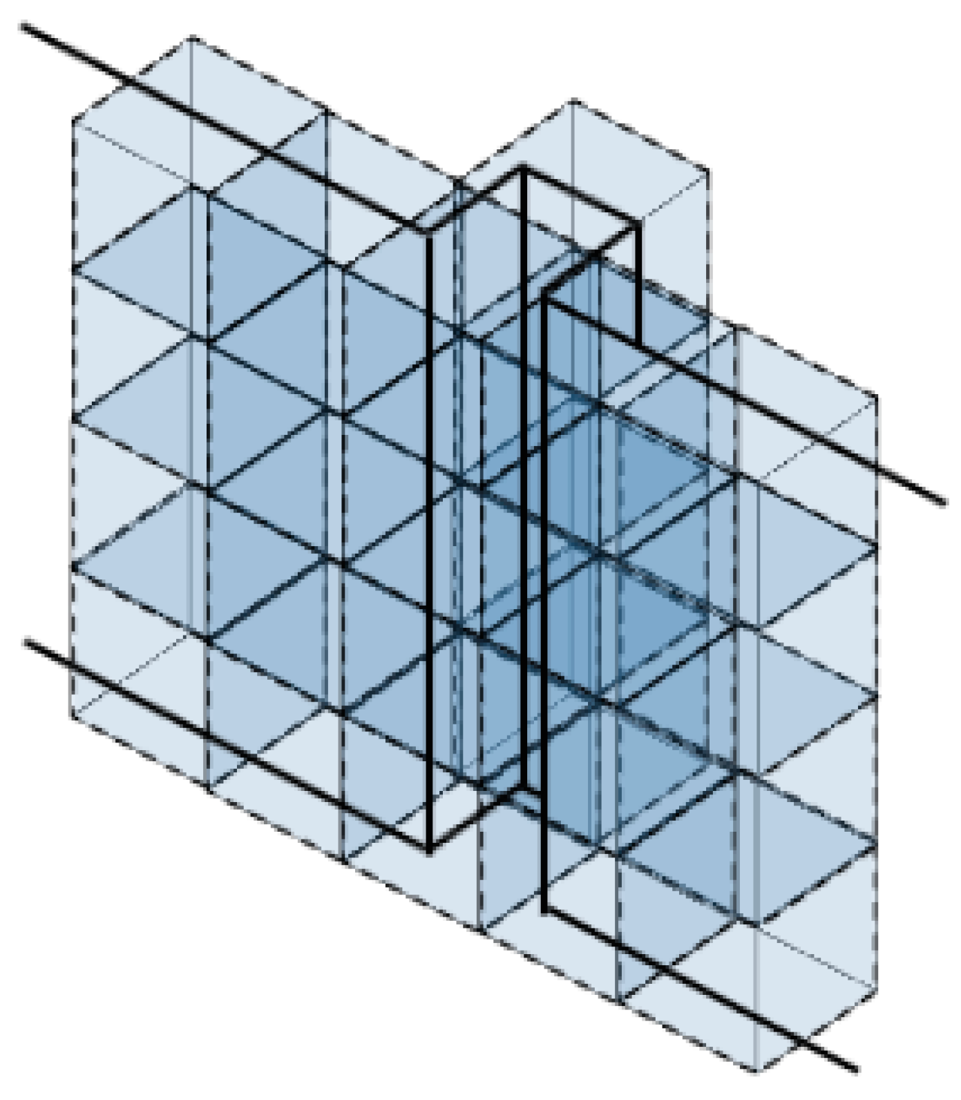
The object sizes of the space and equipment must be adjusted to apply the multi-resolution cube grid method to the data acquired through a 3D laser scanner. This is because the unit sizes (n) must be identical in order for us to check the interference of the space and equipment in the process of dividing them into small nodes using the multi-resolution cube grid method. Figure 1 below shows the node applicable model.

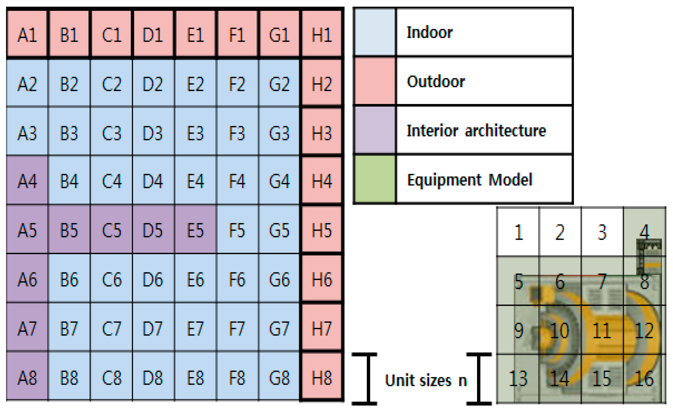
The data simplification process starts first by removing the noises. Noise refers to unnecessary data other than equipment and on-site environmental information (pre-installed equipment, structures, etc.), and the target of noise may vary depending on the purpose. A node exists if data exist at any point in the node in the simplification process based on 3D shape information under the assumption that noises have been removed. This can be checked by referring to cell no.4 of the facilities model in Figure 2. Figure 2 shows a simplified example of transforming space and equipment into grid forms only considering the horizontal and vertical (x, y) coordinates to illustrate the concept. As the final goal of this study was space analysis based on 3D grid method, all three coordinates of x, y, z including the height were analyzed. The grids labeled A1 to H8 in Figure 2 represent the total space of the site environment for equipment installation indicated as grid, and grids labeled 1 to 16 illustrate an example of converting the equipment to be installed into 3D grids.

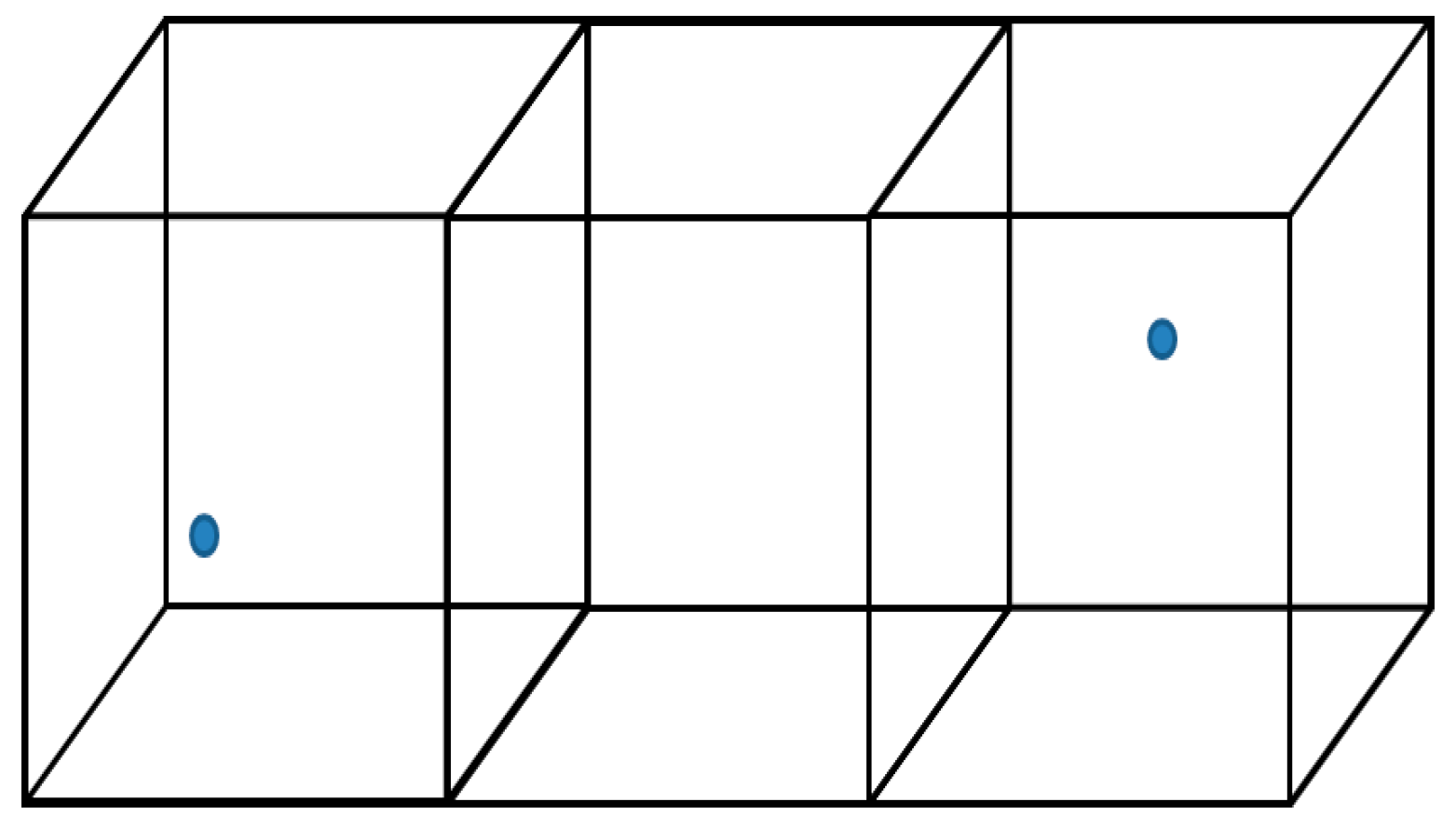
There are a few constraints in deciding the unit size (n) of the node. In collecting point cloud, the point count size, accuracy, and time vary depending on the resolution of instrument used. In this study, a Leica C5 laser scanner was used and the resolutions were classified into High, Mid, and Low. Using the instrument as a reference point, the resolution of the laser scanner was classified into High, Mid, or Low according to the point interval that can be obtained at a distance of 100 m from the reference. In case of Leica C5 used in this study, the accuracy is Low when the point interval obtained from the 100 m distance was 20 cm, Mid accuracy when interval was 10 cm, and High accuracy when the point interval was 5 cm. This study divided the space into grids and recognized unoccupied space by identifying whether a point was included in the grid or not. Consequently, as in Figure 3, the resolution affected node size setting since error of recognizing as an empty space can occur if the node size is smaller than the interval of the points from 100 m distance

If the node size is smaller than the size of the photographing resolution in the used equipment, the following problem arises. The left and right nodes among the three nodes in the figure are perceived as effective because they contain points, but the middle node is perceived as non-existent because it contains no point.

However, the time required for checking the space sharply increases if the node size is diminished to a degree that the distance between points is considered in the actual experiment. If the node size is halved in the process, the number of objects perceived in the test increases by eight times. Therefore, choosing an appropriate node size is critical in algorithm optimization.

3.3. Space Matching Condition Setting

The space and various equipment are matched after the equalization of the unit size of space and equipment. Matching is considered in four conditions depending on the existence relating to relevant data of the space and the equipment. Matching is possible for every node except for those where both of the space and equipment data exist as shown in

Table 2. Matching conditions, space, and unit.

Space	Unit	Matching to Availability	Matching Example (Figure 3)
			Space	Unit
◯	◯	Available	A2	1
◯	●	Available	A2	5
●	◯	Available	E5	1
●	●	Impossibility	E5	5

◯: data absence/●: data exists.

.

The node that represents the location of the equipment in the space must be set before matching. Using Figure 2 above as an example, node 1 of the equipment is used, and this is named as the “reference node.”

The matching of space and equipment depends on which node is the reference node. In the example shown in Figure 3, the nodes of the space where the node no.1 of the equipment can exist are 25 cases in the range of 5 (total horizontal length of the space–horizontal length of the space occupied by the equipment + 1: 8–4 + 1) horizontal cells, and 5 (total vertical length of the space–vertical length of the space occupied by the equipment +1: 8–4 + 1) vertical cells, and the height condition must also be considered. However, there is no additional node at which the reference node can exist by the height setting because different equipment is installed on the ground of the space except in special cases. After the length/width/height conditions of the equipment are set, the reference nodes are moved in equipment rotation. The considered equipment is rotated in four directions. Thus, 100 areas must be checked, which is four times the 25 areas that were set above.

3.4. Implementation of Space Matching Algorithm

The engineering software “MATLAB,” developed by “Math Works,” provides functions that enable numerical analysis and programming environment. MATLAB supports calculations based on a matrix and provides such features as floor plan figures with functions, data, and algorithm implementation through relevant programming. For these capabilities, MATLAB was used in this study to implement the space matching algorithm as discussed above.

The space matching process implemented through MATLAB is as follows:

(1)

Set the range of space coordinates—the size of the total coordinate system must be defined and checked before applying 3D grids. Therefore, the maximum and minimum values of the coordinate system must be set.

(2)

Apply 3D grids—this process checks if there is any point cloud that is classified as data in the corresponding block when applying the 3D grids. If there is point cloud data in the block, the block is wrapped around by colored surfaces for visual identification.

The scan data are segmented by the unit values defined by the user, and the existence of data in the segmented node is determined, in which case the node is marked as having data.

Table 3. 3D grids algorithm application.

Point Cloud Data	3D Grid Data (Transparent Data)

below shows the results from that process.

(3)

Apply the matching verification algorithm—the algorithm for verifying the possibility of matching is applied using the 3D grid application data outlined in the previous step.

The algorithm for verifying the possibility of matching is applied as described above using the data created from the 3D grids in the previous step. Space data must be matched at the bottom because different equipment is installed on the floor of the space. For equipment data, all the data must be included in the algorithm because every node that has data must be checked.

Next, the equipment data are moved to the first node of the space model and matching is checked. When the matching process is started, the parameter FailCase is set and one is added to this parameter whenever the matching fails. The FailCase value is checked at the end of matching verification. If this value is 0, it means that every matching is successful. In this case, the corresponding matching coordinate is saved in the text file to which the results are outputted and the algorithm moves on to the next matching node. On the other hand, if the FailCase value is not 0, the algorithm moves on to the next matching node without saving the node coordinate in the text file. 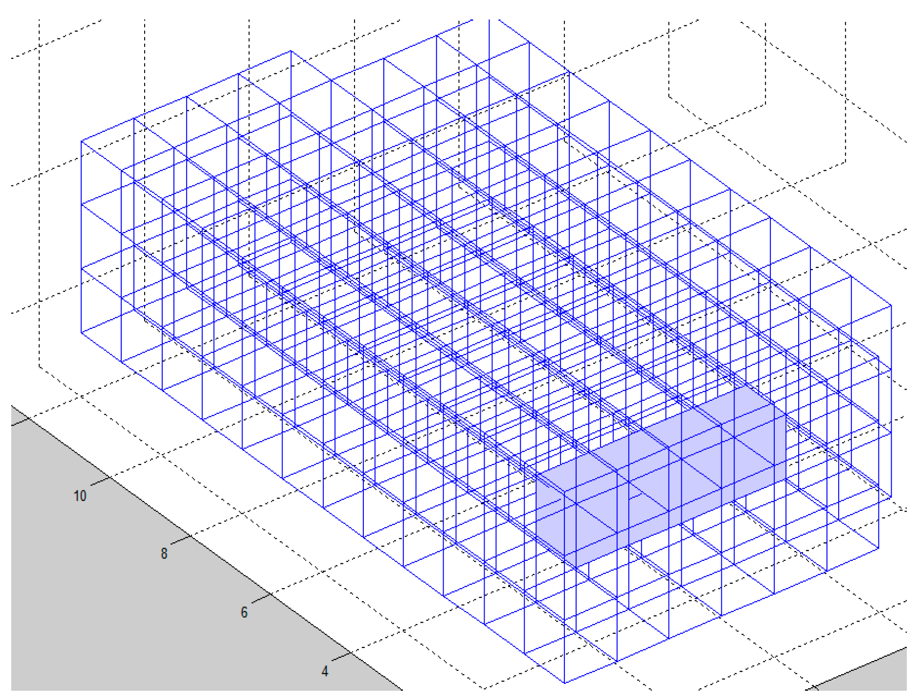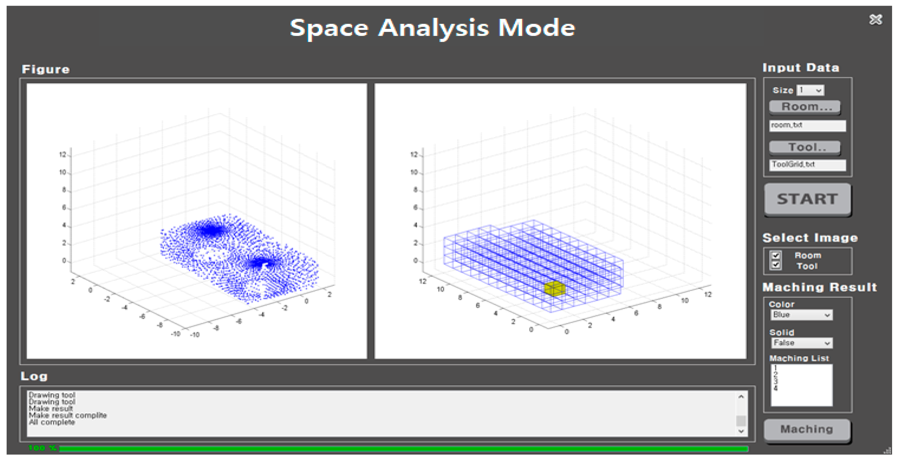Figure 4 shows the result value outputted after verification by the matching algorithm. The coordinate pairing occurs in the horizontal direction. From left to right, the user-defined unit value, x coordinate, y coordinate, and z coordinate are displayed. The figure also shows the visual expression of one of the coordinates that can be matched. For space data, only the edges are outputted for visual expression. The facilities data are outputted by colored surfaces.

3.5. Software Configuration

In this study, basic algorithms of numerical analysis and space analysis were pre-applied in MATLAB, and finally the C#-based space analysis system was constructed. This space analysis software is divided mainly into five areas: Input Data indicating the data setting value area for spatial analysis; Select Image indicating the execution results editing area; Matching Result indicating the execution results refresh setting area; Log showing the processing contents being performed; and Figure which is configured to select the data for spatial analysis and input the value while showing grid generation and spatial analysis numerically. Figure 5 below shows the space analysis software.

3.6. Pre-Processing for Data Optimization

Converting the point cloud data into grid system is essential for space analysis. However, point cloud data collected through laser scanning is large in volume and requires considerable processing time for converting. As such, this study proposed a pre-processing method based on sub-sampling which can optimize the point cloud data prior to space analysis and verified the applicability thereof by comparing the accuracy.

As an actual space for optimizing spatial analysis data, a room size of 2.5 m × 9.4 m × 2.6 m was selected and an as-built model reflecting the shape of space was created through laser scanning. Through the Leica C5 laser scanner, the shape information of the room was obtained in the form of a point cloud, and the final output was generated in the pts format through matching work and format conversion (Leica Cyclone Software: Cyclone).

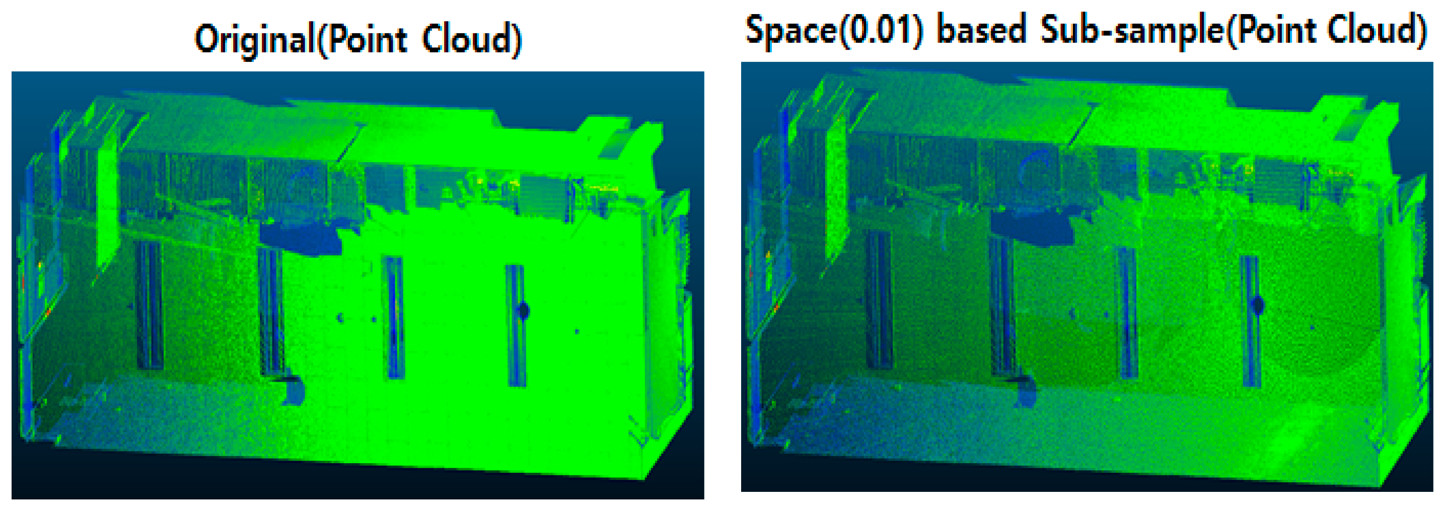
Sub-sampling of point cloud data was performed first for data optimization. Sub-sampling refers to a function that sets the user’s desired space within the space consisting of points and reduces several points in the set space to a single point. It is used to reduce the load for handling and loading of massive point cloud data and to reduce the data volume. The data collected through laser scanning resolution set at Mid, has the capacity of 259 MB and consists of total 14,317,597 points. Increasing the resolution in the laser scanning step increases the capacity and number of points. Figure 6 below shows the example of sub-sampling.

Sub-sampling was performed using open software “Cloud Compare,” and the space interval was set to 10 cm, which was lower than the grid box size provided by the space analysis system. Sub-sampling output capacity was reduced to 27.4 MB and the total number of points was reduced to 705,478. By comparing the processing time of space analysis system for the original data and the sub-sampling data respectively, the applicability of the optimized data (light weight) through sub-sampling was verified.

Table 4. Comparison of original data and sub-sampled data for data processing.

-		Original Point Cloud (14,317,597–259 MB)		Sub-Sampled Point Cloud (705,478–27.4 MB)
-		time	Result	time	Result
Data Analysis	Box size (1.0 m)
		66 s	20 ea	8 s	20 ea
	Box size (0.7 m)
		114 s	74 ea	15 s	74 ea
	Box size (0.5 m)
		416 s	103 ea	27 s	103 ea

below summarizes the comparison results of processing time using the original data and the sub-sampled data and the resulting values respectively. The original data and the sub-sampled data were tested for the grid box sized 1 m × 0.7 m × 0.5 m in the space analysis system, respectively.

In case of the original data, it took 168 s to load the data. When the space analysis was performed, it took 66 s for the grid box size 1 m, 114 s for box size 0.7 m, and 416 s for box size 0.5 of the respective set values. For the sub-sampled data, it took 7 s for data loading (−161 s compared to the original data), and it took 8 s for grid box size 1 m of the set value (−78 s compared to the original data), 15 s for box size 0.7 m (−99 s compared to the original data), and 27 s for box size 0.5 m (−389 s compared to the original data) of the respective set values. When the space analysis results were compared, both original data and sub-sampled data showed the same resulting values with 20 each for box size 1 m, 74 each for box size 0.7 m, 103 each for box size 0.5 m respectively. In the space analysis system, the sub-sampling technique was used to optimize and minimize the amount of input data, and as a result, the same resulting values as the original data were acquired within the shortened processing time, verifying its suitability.

3.7. Software Verification

An experiment for securing installation space for a virtual equipment in a space of a simple shape was conducted before applying the developed algorithm to an actual site. Virtual equipment with the size of 1(m) × 1(m) × 4(m) were applied, which simplified the unit node value to 1 (m) (Grid Box Size 1 (m)) for the convenience of calculation in order to check the difference from the actual calculation. Furthermore, the unit node value of 1 (m) was also applied to the target space as described above. The calculation and algorithm applications were carried out without the rotation of equipment because the present calculation was a process of merely comparing two resulting values, rather than requiring the number of all equipment arrangement spaces.

Next, the corresponding space data was applied to the developed algorithm and the results were checked. Examples of these results are shown below in

Table 5. Experimental results using a virtual appliance.

Node Size	x	y	z
1	0	6	2
1	0	8	2
1	2	10	2
…	…	…	…
1	14	8	2
1	14	10	2

.

Table 5 shows the coordinates (x, y, z) of the grid box where the virtual equipment is located within the 3D grids of the entire site enabling to obtain coordinate values in which the virtual equipment can be arranged within the site. The node size represents the grid box size. If point cloud was found within the box of node size defined by the algorithm, the xyz coordinate value was used to store the location.

The sample results obtained from the algorithm and the calculation results for the number of spaces that can be actually arranged were compared and outlined in

Table 6. Calculate for the verification of the algorithm.

Experiment	Calculated	Algorithm Results
1	29	29
2	21	20
3	18	18

. To compare and organize the number of spaces available where equipment can be arranged, the resulting sample value through algorithm calculation which was made based on the box volume that equipment occupies, was compared with the computed number of space where true arrangement of equipment is feasible.

In experiments 1 and 3, the two results are identical, but they are different in experiment 2. This problem appears because the starting point for applying the algorithm is different from the starting point of the calculation process. If the two starting points are identical or the reference node value is lowered, the same results are obtained.

4. Case Study

As a case study, the acquisition of shape information and registration were performed on three interior/exterior spaces and two types of equipment using the proposed method. An example of these spaces is shown in Figure 7. This example space is a photograph of an indoor plant that is actually in operation. Specifically, the indoor plant used for the case study was the underground plant room of the Multi Research Lab #2 located at the Natural Sciences Campus of Sung Kyun Kwan University, Suwon, Korea. The equipment considered for the study was two existing boilers with the size of 1 (m) × 1 (m) × 2 (m) (including all connected pipes) housed in the plant room. In configuring the equipment for the study, the protruded surfaces of the boiler due to the external irregularities (i.e., control valves, gauges, etc.,) were included as part of the equipment while external connections, such as connecting pipes were segregated from the boiler in random length and not considered as part of the boiler.

The goal of the experiment was to rearrange boilers’ location within the same plant room so as to install another equipment.

Table 7. Summary of the experiment space and equipment.

Item	Summary
Space Location	Underground Plant Room, Multi Research Lab #2, Natural Sciences Campus, Sung Kyun Kwan University
Type of Equipment	Electronic Water Heater Boiler (2 ea.)
3D Grid	1 (m) × 1 (m) × 2 (m)	1 (m) × 1 (m) × 4 (m)
Case Study Goal	Rearrange boilers’ location within the plant room to make space for another equipment

below summarizes the space and equipment information of the case study.

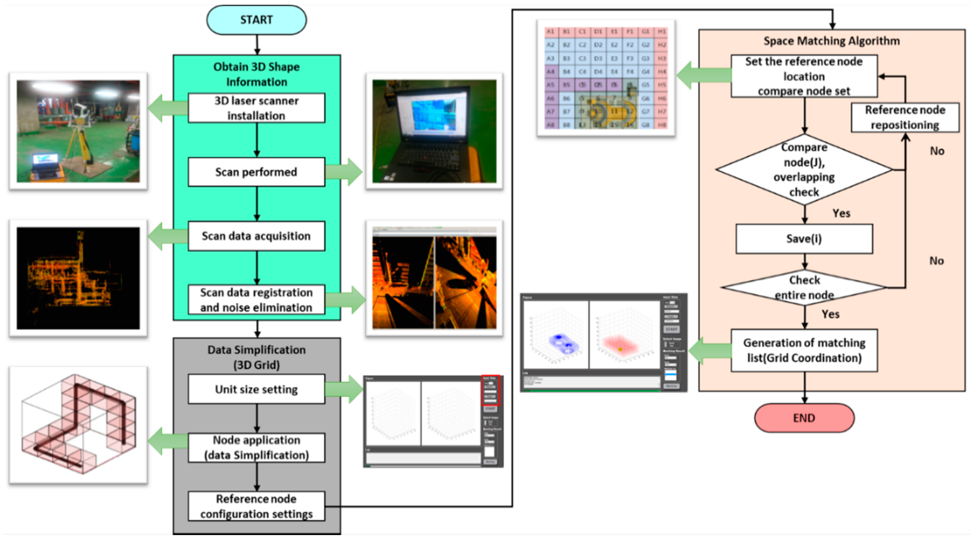
The case study experiment was conducted based on a three-step process: (1) build 3D shape information, (2) perform 3D data simplification, (3) apply space matching algorithm and analyze space to place the equipment. Figure 8 shows these steps and the algorithm process involved in the case study.

Specifically, 3D shape information was constructed in the first step by first acquiring the 3D shape information using laser scanner, registering scanned data, and then by removing noises. In the second step, 3D data simplification was accomplished through unit size setting, 3D grid data conversion (data simplification) for node application and setting the reference node. Finally, space arrangement was performed in the third step by applying space matching algorithm and analyzing space.

The 3D grid method described above was applied to convert the data for calculating the space and equipment point clouds. This process is shown in Figure 9.

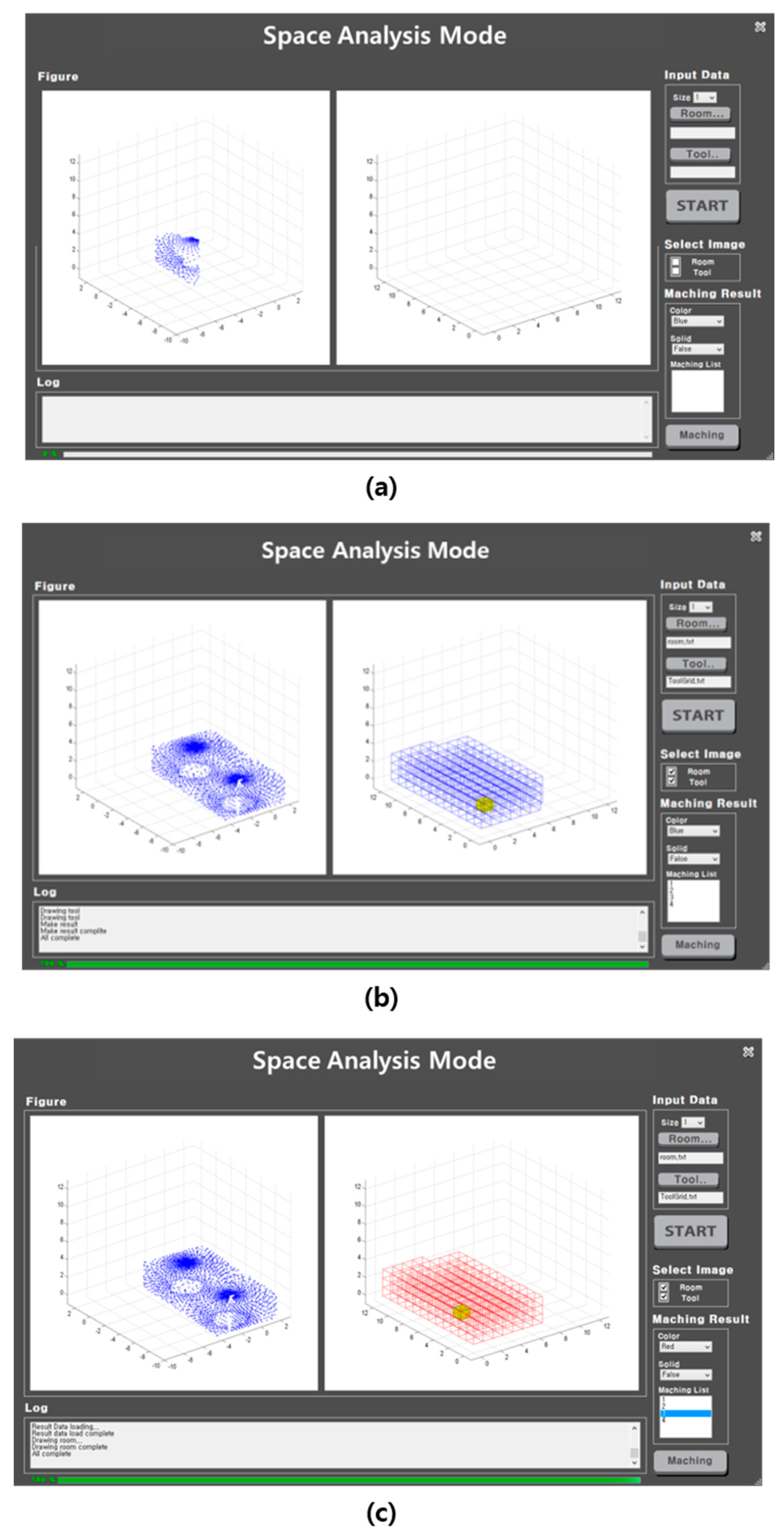
Figure 10 shows the software processing sequence. Input data can be divided into four configurations: the setting part to configure the grid box size to perform the space analysis; the input part to add point cloud data of the space to be analyzed; the tool part to set the starting coordinate point for installation; and lastly the start part to perform the final algorithm and calculation. The user first sets the grid box size according to the accuracy to be obtained and inputs the shape information data collected through the laser scanning operation. Thereafter, the data for setting a required space are further added to start the calculation.

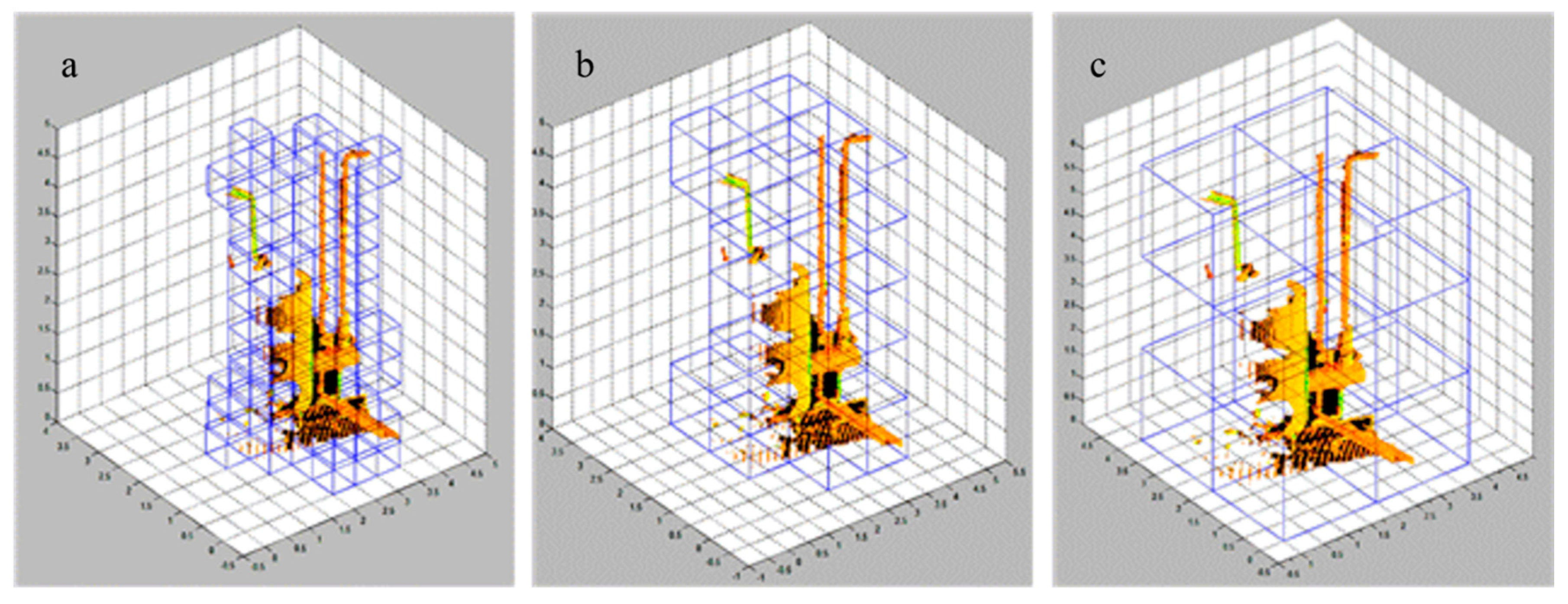
The matching experiments were conducted using a total of three types of node values for two types of equipment and three different space types. Figure 11 was classified by node size (grid box size), which was set to 0.5, 1.0, and 2.0 m.

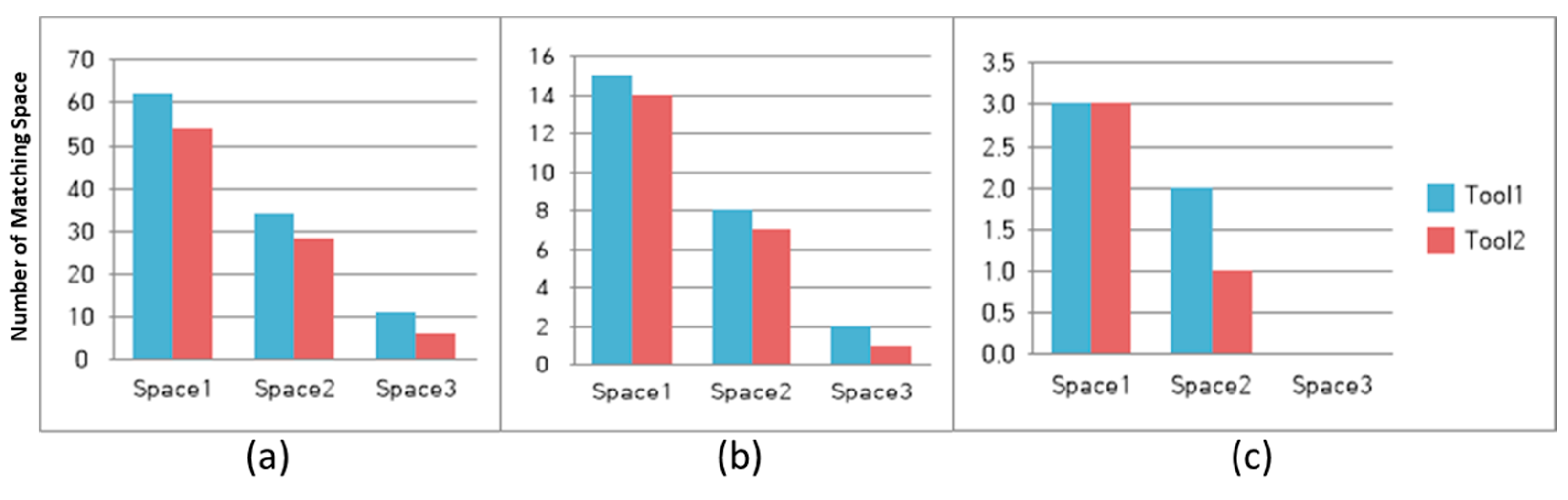
The equipment and space transformed into 3D grids were matched through the above process, and the results were calculated. The results are shown in Figure 12. The numbers on the graph represent the number of points in which the correlated spaces (indicated as Space 1, Space 2, and Space 3) and equipment (indicated as Tool 1 and Tool 2) in the algorithm matched.

The resulting experiment shows that the number of valid spaces that can be used for allocating equipment varies depending on the node size (i.e., size of the grid box). We have searched the valid installation spaces for equipment as follows: in case of space 1, tool 1 (equipment 1), 62 each (node size 0.5 m), 15 each (node size 1 m), 3 each (node size 2 m); in case of space 1 and tool 2 (equipment 2), 54 each (node size 0.5 m), 14 each (node size 1 m), 3 each (node size 2 m); in case of space 2 and tool 1 (equipment 1), 34 each (node size 0.5 m), 8 each (node size 1 m), and 2 each (node size 2 m); in case of space 2 and tool 2 (equipment 2), 28 each (node size 0.5 m), 7 each (node size 1 m), and 1 each (node size 2 m). In case of space 3, tool 1 (equipment 1), 11 each (node size 0.5 m), 2 each (node size 1 m), and 0 each (node size 2 m); in case of space 3, tool 2 (equipment 2), 5 each (node size 0.5 m), 1 each (node size 1 m), and 0 each (node size 2 m) were searched. In case of space 3, the valid spaces were found at node sizes (grid box sizes) of 0.5 m and 1 m, but no valid space was found at 2 m or more. If a detailed aspect of space analysis needs to be considered, the smaller the grid box size, the more the available spaces. However, because of the increase in space analysis processing time, it is necessary to consider the size of node only when intending to identify whether an equipment can be installed or not.

5. Conclusions

Industrial plant projects are characterized for their extra complexity due to their functional characteristics. Many problems occur during the operation and maintenance stages mostly because the installation spaces of the required equipment are not laid out in an efficient way. This study is aimed to resolve the problems that occur in the actual installation process caused by the differences between the installation of additional equipment and the original floor plans during and after plant construction. In this process, the two types of 3D shape information, space model and equipment model, were matched through the 3D grid method based on the existing research data about the 3D shape information. A method for checking the overlap of the two data sets was proposed. Two algorithms for matching the 3D shape information were created: one for the simplification of the target installation space and equipment using the 3D grid method, and one for verifying the overlap of the two types of simplified shape information. Then the integrated matching algorithm was developed. The algorithm was implemented in such a way that it can be verified in the two forms of text and visual image. Actual site data were applied to the algorithm and the effect was verified in this process. Discrepancies and problems can be resolved in the response measures according to space variations that appear when various equipment is arranged during plant construction. The equipment arrangement space was secured using the algorithm through “MATLAB” and this is verified in two forms of text and image.

In this study, the process to convert the point cloud data into the 3D grid was essential, which took the most time. Therefore, in order to optimize the 3D grid conversion process, this study proposed a pre-processing method based on the sub-sampling that optimizes (reducing volume) the point cloud data. The study further applied the original point cloud data and the sub-sampled data within the same space to the algorithm and program and verified the validity through comparing the resulting values and the processing time.

Finally, after verifying the algorithm, a program composed of a total of five areas which enables the C# based data setup, editing, and analysis, etc., was constructed. Based on this, space analysis and valid space search were performed for the arrangement and installation of two types of equipment with different dimensions (1 m × 1 m × 2 m and 1 m × 1 m × 4 m) in three different spaces. As a result, information on the valid space for the equipment arrangement according to the varied node size (i.e., grid box size) was obtained.

One of the limitations of this study is that it has not been applied to plant sites with irregular characteristics. Furthermore, the value of the unit size of the node for the 3D grid application used by the algorithm is left to the user of the algorithm. Therefore, the application of this algorithm requires long-term experience in plant sites or skilled experience if it was to be applied in a variety of cases.

Finally, this study constitutes a starting point of space-matching system based on a mathematical model and space-matching software to assist during the decision-making process. In addition, the proposed algorithm is expected to be established as the base system for various research projects. Through additional future researches, it is expected that the limitation of space-matching system can be solved by application and expansion of technologies such as editing and optimization based on point cloud viewer.