Sustainability of an Activity Node in Global Supply Chains

Abstract

Urban shrinkage is a remarkable phenomenon that cannot be convincingly explained by existing theories on urban growth and is closely linked to the global supply chain (SC) nodes in the labour market. This paper shows how a municipality in which an activity SC cell (production or service) is located as a node in the SC graph can be made more attractive for industrial activities and human resources, more sustainable, and less shrinking, through appropriate tax policies and investments in the infrastructure of the central places—cities where production or services are located. To this end, we developed the decision support model for the joint control of urban rightsizing by SC managers and local authorities. In the model we linked the extended material requirements problem (MRP) with a normalised asymmetric gravity model. The paper outlines how local authorities and institutions, when planning for the growing intensity of production or services, in a city where the number of workers is insufficient, should take into account the impact of taxation as well as investment in the infrastructure of a municipality, and not just net wages, in order to attract human resources. They need a decision support model for their negotiations on the rightsizing of the city. The objective was to develop a model of fiscal mechanisms in the interactive decision making processes of local authorities and SC managers to control the availability of labour in the city where production or services are running and need to grow because SC managers want to increase production or services but the available labour force is shrinking. A case study in Slovenia shows how local authorities and SC managers should work together to maintain a sustainable activity cell in a functional region of the urban agglomeration where this production or service is located. It models how to plan the rightsizing. Such an integrated policy best achieves the desired intensity of the supply chain, thereby avoiding the relocation of activities outside the region, which allows unsustainable flows of human resources and uncontrolled shrinking of a city or region.

1. Introduction

Shrinking Cities

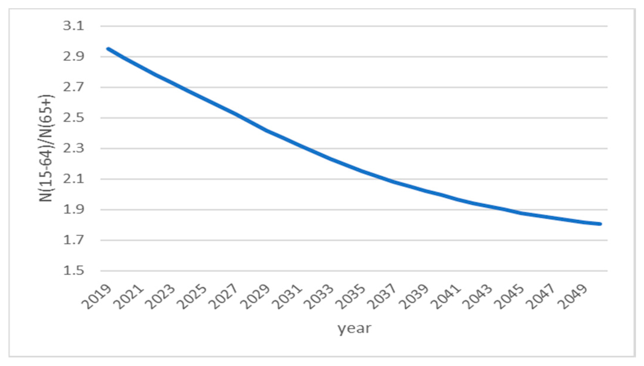
The European Union (EU) is expected to lose 49 million people of working age (15–64) over the next 30 years, as shown in Figure 1. The ratio of the working-age to the population aged 65+ in the European Union will fall from over 3 in 2020 to 1.6 in 40 years (see Figure 2). In many cities, this decline is expected to be even greater. There is a long list of definitions, indicators, and causes of shrinking cities [1,2,3]. The most recent overview is given in detail in [4]. According to the Shrinking Cities International Research Network, shrinking cities are defined as “urban areas with a minimum population of ten thousand residents that face population losses in large parts for more than two years and are undergoing economic transformations with some symptoms of structural crisis” [5,6]. We consider this definition to be too narrow, as it is limited to the population decline inside urban areas, without taking into account their larger area organised around the city as a central place (see Figure 3 and Figure 4).

It is foreseeable that in the case of a scenario without migration (non-migration, NMIGR) Europe will lose 120 million more inhabitants within 100 years than in the baseline scenario (BSL). From Figure 1 and the same data sources there follow Figure 2. The declining ratio between the working-age and population aged 65+ in the European Union declines faster in shrinking cities and in case of the no-migration scenario (BSL scenario).

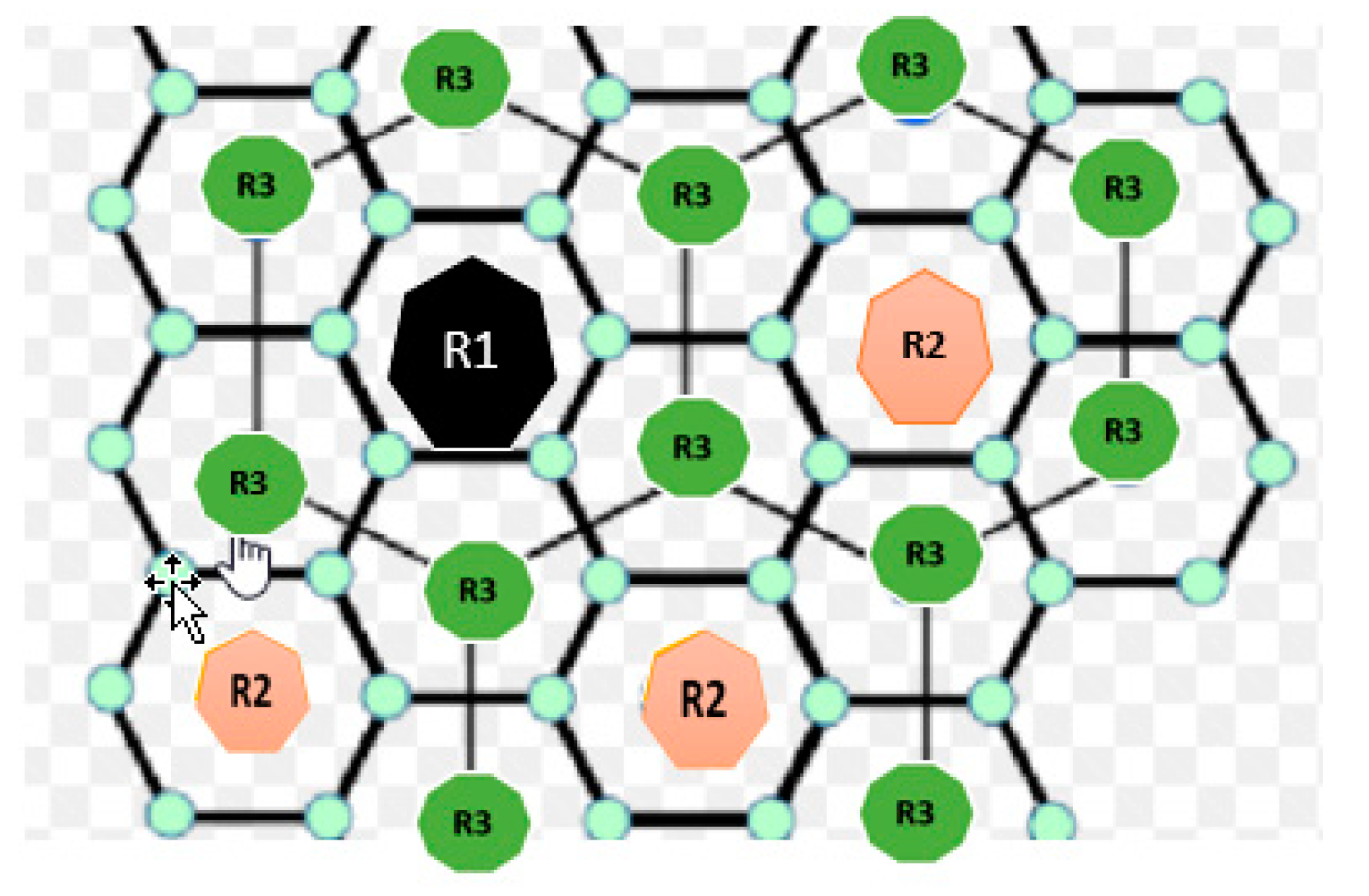
The concept of the central place comes from the theory of central places (CPT), which tries to explain the location of human settlements in a system of urban agglomerations, their size, and number in a landscape. The theory was first developed by Walter Christaller [7], who explained that settlements are “central places” that provide services and employment to the surrounding areas. In these central places are the nodal points of many economic and social activities. There could also locate nodes of global supply chains. According to CPT, the ideal surrounding areas form embedded hexagons, as shown in Figure 3. These ideally embedded tessellations are changing their shape, i.e., their demarcation delineation curves, due to some geographical, social and economic constraints. Throughout history, these surrounding areas have often been managed as separate administrative units, as in Europe the regional units on various levels (Nomenclature of territorial units for statistics—NUTS) at the levels NUTS 1 to NUTS 3. These regions are defined by the government and are called formal regions.

According to Christaller’s CPT, a central place is a city or a town as a node of a region (in Figure 3, there are cities, R1, smaller towns, R2, and/or even smaller towns, i.e., market towns, R3), where a node of a global supply chain can also be located. Cities, R1, also cover the areas of the hexagons that belong to the nearest towns, R2. Each town, R2, also hierarchically covers the areas of the hexagons that belong to the nearest market towns, R3.

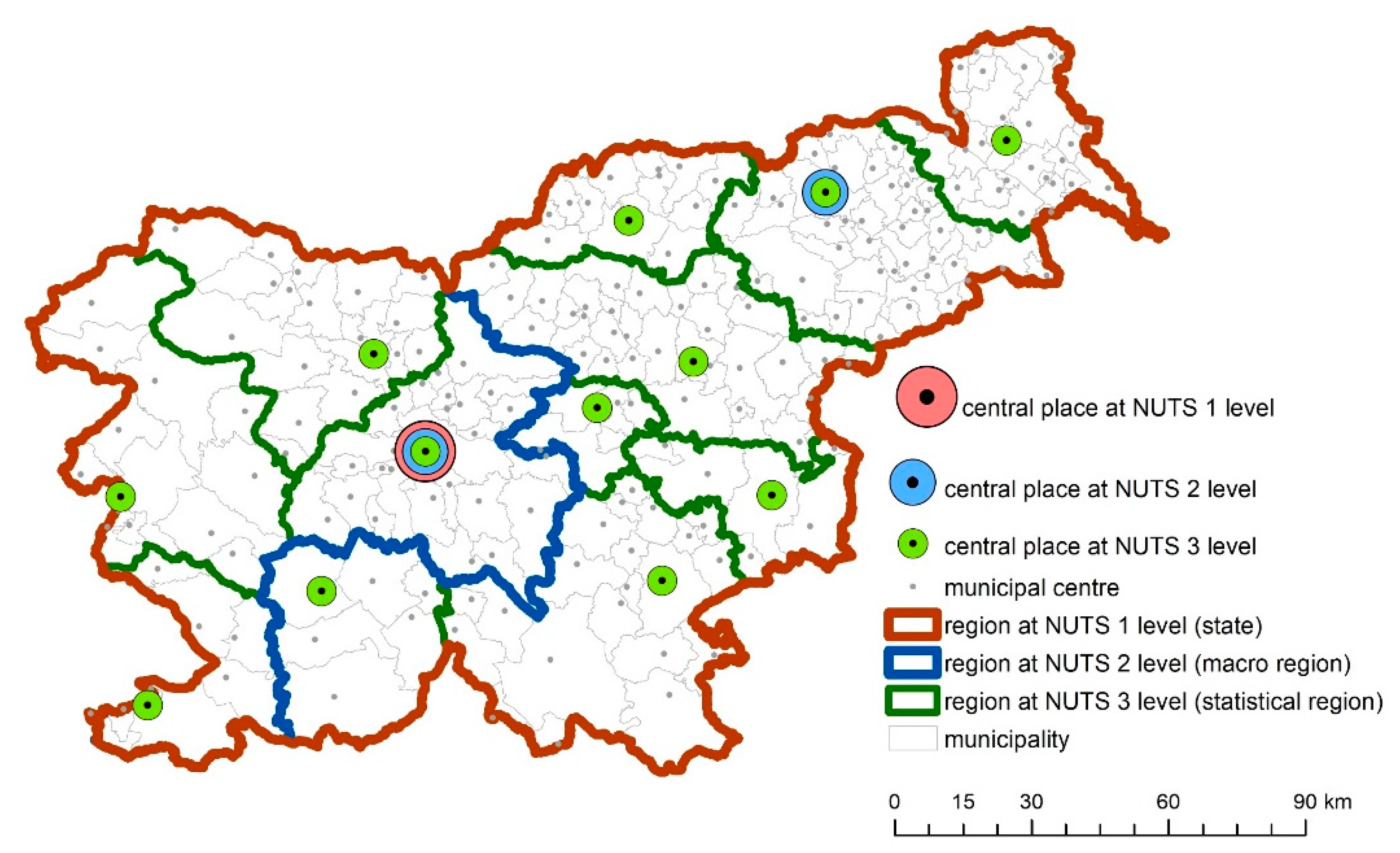
In Slovenia, this hierarchical structure, which shows NUTS 1 (state) level with the central place Ljubljana, NUTS 2 level with the central places Ljubljana (governs Western Slovenian Region) and Maribor (governs Eastern Slovenian Region) on the lower level, and the central places of the NUTS 3 regions, is shown in Figure 4. Geographic and political influences greatly shifted the edges of their surrounding areas from hexagonal shapes to something else.

CPT tries to show that each urban settlement is held in place within a system of cities, and it follows that any change in its boundaries is determined by the position of a place within the system [8]. During demographic growth or decline and during urban development, technological and economic constraints change the position of a place within the system, even if the demarcation curves of the formal regions and their administration remain unchanged. Formal demarcation is often less flexible because it is dependent on administrative demarcation based on political, historical, spatial relations. However, the influences of demographic and economic changes force the economic interaction flows.

Under the changing influence of technological and economic factors, new demarcations emerge, which in the case of the non-changing formal regions form so-called functional regions (FRs). Therefore, a functional region is assumed to be the territorial unit resulting from the organisation of social and economic relations. The demarcation curve between two functional regions is a threshold at which the economic or social relations with two regions are equally strong. Changing effects of technological and economic factors also influence the shrinkage or growth of cities.

Functional regions include, for example, the reception area of a service station, the area from which school children gravitate to school, a trading area of a shop, or the area from which workers are most likely to commute. Consequently, FR is the topic of our modelling and decision-making formalization, which is presented in this article.

While we have found a little more than 20 articles from the last century that mention shrinking cities, a whole corpus of literature on shrinking cities has been produced since the beginning of this millennium, from 84 articles in the first decade to an average of 132 articles per year over the last five years; these describe the nature of the challenges associated with urban population and economic decline.

This decline affects cities around the world. The literature focuses on shrinking cities in the United States [9], the European Union [10], and Japan [11,12]. The articles have been published in numerous scientific journals since 2012. At that time, the first paper was published in Sustainability [13]; there are 43 more such papers in the same journal. The articles attempt to explain the reasons for shrinkage and to prescribe appropriate solutions to spatial planners and other professionals to potentially mitigate it. The authors explain the causes as low fertility, reduced industrialisation, and the fall of the Iron Curtain. According to academic discourse, there are many causes of this shrinkage, its indicators, and the measures to be taken. These are listed in

Table 1. The main generators of shrinking cities, indicators, and remedial measures given in the literature.

Generators	Indicators	Measures
○ Low fertility ○ Deindustrialisation ○ Globalization ○ Pollution ○ Natural disasters ○ Wars and revolutions ○ Suburbanisation ○ Dissolution of states, like after the fall of the iron curtain ○ Changed transportation networks	○ Population loss ○ Ageing of population ○ Empty houses ○ Economic downturn ○ Poverty concentration ○ Urban land rent decrease ○ Real estate value decrease ○ Intrusion of local taxes ○ Disinvestment ○ Over-capacitated infrastructure ○ Unemployment	○ Rightsizing in spatial planning ○ Greening/urban farming ○ Gentrification ○ Investments in social infrastructure ○ Demolition ○ Land management ○ Support of art and tourism ○ Public–private partnerships ○ Subventions to industries ○ Support of social enterprises ○ Increased accessibility ○ Improved logistics

.

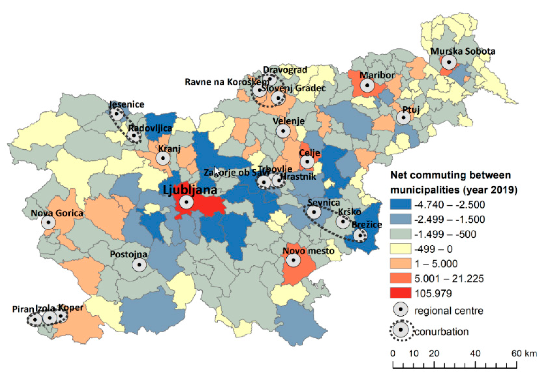
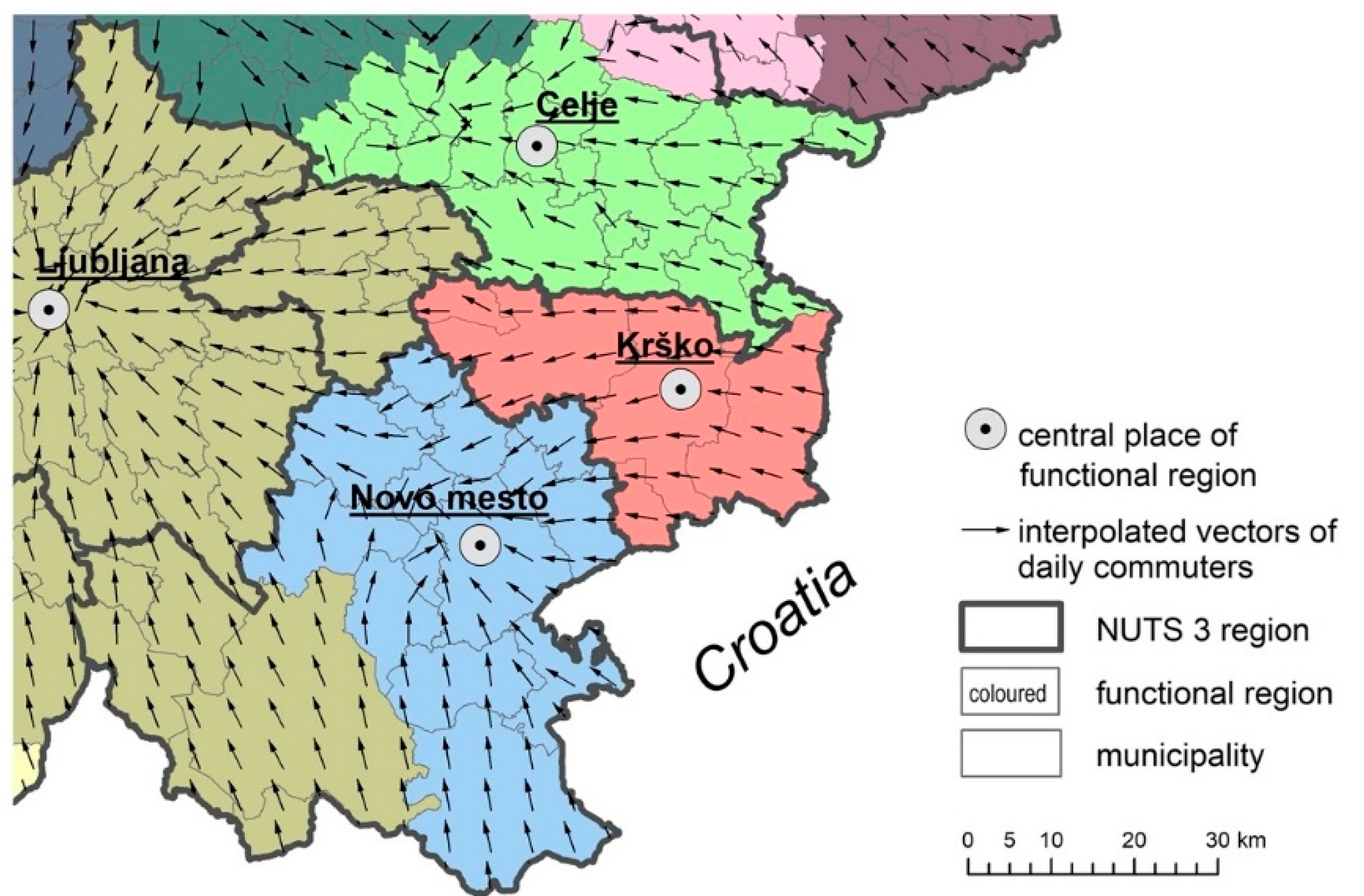
Figure 5 shows the shrinkage of one of the Slovenian administrative regions on NUTS 3 level—the Posavje region including its central place—the town of Krško. NUTS 3 regions in EU are regions established for specific purposes, e.g., for statistical reporting. The geographical location of the NUTS 3 regions, the functional regions at the macro level as well as the central places of the regions in the south-east part of Slovenia is shown in Figure 6. In 20 years, the Posavje region would lose 20% of the working population and half of this cohort in 50 years according to the non-migration (NMIGR) scenario. The main competing city is Novo mesto with its blue functional region. The fiscal policies of the two central places, the public amenities there and the salaries in their production and services’ nodes (industrial activities in Krško and Novo mesto) determine which city more inhabitants will commute to and migrate to, and thus influence the movement of the demarcation curve between these two colours when the administrative regions on NUTS 3 level do not coincide with the functional regions.

The literature on the reactions of professionals to shrinkage looks for the method of rightsizing. Articles such as those by Temeljotov-Salaj et al. [14] and Slabinski [15] emphasise the importance of greening through infrastructure and urban agriculture on vacant public land. However, our intention, was to consider a different approach. We planned to develop decision-making models and find solutions through closer cooperation between the local authority (local taxes and subsidies, investments in infrastructure) and the managers and owners of the supply chain whose supply chain (SC) activity cells (production or services) are located in the city concerned (wages and benefits).

Our main objective is to further develop the combination of extended material requirements problem (MRP) model, which allows the projections of the flow of goods in a SC and the gravity model, which allows the study of the availability of human resources in an activity cell of a supply chain as a node of a chain located in the analysed city, a city that risks losing a significant part of its population in a few decades. We are developing this composite model in order to be able to study the impact of different policies, especially fiscal and wage policies, on the growth or shrinkage of the city. In short, we want to study the effects of an integrated urban policy and supply chain management, which have their own cells for production or service activities (factories, services) in the city concerned, on sustainable, programmed growth or shrinkage. The final answer will be what a dynamic rightsizing of city should be to keep the SC activities and population size in the region; how to support the decision-makers with a proper model?

By combining fiscal policy and wage formation policy with investments in social infrastructure, we propose an answer to the question of how the desired sustainable growth or decline of a city and its functional region (FR) can be achieved, taking into account the chosen dynamics of flow intensity in supply chains with activity cells in the city. The regulated rightsizing of a city FR was modelled by further developing and coupling two models: the material requirements problem (MRP) developed by Grubbström [16,17] and the gravity model presented by Janež et al. [18]. A number of fiscal policies and investments in social infrastructure are presented as regulators of dynamic rightsizing, as they were designed in an article for a case where it was assumed that only wages regulate flows [19].

Low fertility as a generator and ageing as an indicator in Table 1 are associated with the declining size of the available labour force. This dynamic is deeply worrying in many European countries. For example, the European demographic projections are characterised by a rapidly decreasing ratio of the working-age population to the population aged 65 and more. Figure 1 shows the projections for the “no-migration” and “migration” scenarios, and Figure 2 shows the rapidly decreasing ratio of the working-age population to the population aged 65 and more. The ratio falls from 2.9 in 2020 to 1.8 in 2050 (Baseline Scenario-BLS). However, this dynamic varies considerably both between countries and between cities and regions within countries, as calculated on the basis of the 2018 Ageing Report: Economic and Budgetary Projections [20] and updated by the statistical office of the European Union-EUROSTAT in 2020 [21].

Such a decline requires the use of labour from the hinterland. In the human resources (HR) market, the costs and timing of commuting from home to work or migration to the city affect the level of wages and/or land rent and the market value of real estate. In other words, these factors influence the total costs of HRs in the supply chains (SCs) activit y cells and, thus, the profit stream generated in a SC. The results related to the daily commuting and migration forecasting models give us significant insights into the planning activities in the central cities of the areas. We calculate these parameters on the basis of spatial interaction models (SIMs—the generic term for various models used to explain movement in space). SIMs range from the basic symmetric gravity model to Wilson’s entropy [22]. In Section 2.1, we present our development of the normalised asymmetric gravitational approach with the acronym NE_SIM and link it to the activity cells of a SC as nodes in a global SC where a production or services of this SC are located.

2. Method

2.1. Normalised Asymmetric Gravity Model

The model used in our study is an improvement of the general SIM model developed by Cesario [23]. It is asymmetric and includes factors that have been found significant (p < 0.001) for the attractiveness or stickiness of a spatial unit. We have extended the model [23], considering also [24] to analyse the effects of real estate taxation and social infrastructure investments on the attractiveness and stickiness of a municipality. Let us use the following notation, as given in

Table 2. The basic notation in the NE_SIM formalisation.

Notation	Meaning
$C_{ij}$	Daily commuting flow from i to the considered FR$j$
$M_{ij}$	Annual migration flow from i to the considered FR $j$
$X({\tau }_{i,j})$	Relative distance to the average of the economic space between regions $i \mathrm{and} j$
$X{(\kappa )}_i$	Coefficient of factors $\kappa$ in the origin $i$, relative to the national average
$X{\left(\kappa \right)}_j$	Coefficient of factors $\kappa$ in the destination $j$, relative to the national average
$c\left(C\right);c\left(M\right)$	Calibration parameters
$\kappa =POP$	Population size coefficient
$\kappa =UEM$	The unemployment rate, relative to the national average
$\kappa =w$	Gross personal income rate, relative to the average of the studied area
$\kappa =DWE$	Number of dwellings per inhabitant, coefficient of the average for the studied area
${\left(1+q_{\chi }\right)}_i$	The factor of changes in relative property taxes in i (for example: if the property taxes increase for 15%, then ${\left(1+q_{\chi }\right)}_i$ = 1.15)
$\kappa$= rev	The municipality’s budget per capita, relative to the national average
$\kappa =V$	The housing market price [€/m2], relative to the national average
$\epsilon$	The negative parameters characterising the distance friction (power of distance)
${\left(1+q_w\right)}_i$	The factor of changes in relative wages in $i$
α	The power of origin to push the migrants from this origin (stickiness of an origin)
β	The power of destination j to attract the migrants to this destination (attractiveness of a destination)
γ	The power of origin to push commuters from this origin (stickiness of an origin)
δ	The power of destination j to attract the commuters to this destination (attractiveness of a destination)

.

The model is formalised by Equations (1) and (2) for commuting and (3) and (4) for migration in Section 2.2. The SC model is briefly presented in Section 2.3, and the interaction of flows of human resources HR with the SC flows is formalised in Section 3. In addition, as the most important novelty, we have derived in Section 3 a solution for regulation and control through fiscal and investment policies at wage levels acceptable to supply chain managers so that they do not have to relocate their activity cells elsewhere. This is because the need to increase wages may cause managers to close the activity cell that is part of the SC in the city.

The sum of the commuting inflows $C_{.j}$ from other areas per day to a town of the considered FR$j$ and the sum of commuting outflows from a studied FR$i$ to other areas can be written as follows:

$$C_{.j}=c(C){\displaystyle \sum _{i}X({\tau }_{ij}}{)}^{\epsilon (C)}{\displaystyle \prod _{\kappa \in S}X{(\kappa )}_i^{\gamma (\kappa )}}X{(\kappa )}_j^{\delta (\kappa )}$$

(1)

$$C_{i.}=c(C){\displaystyle \sum _{j}X({\tau }_{ij}}{)}^{\epsilon (C)}{\displaystyle \prod _{\kappa \in S}X{(\kappa )}_i^{\gamma (\kappa )}}X{(\kappa )}_j^{\delta (\kappa )}$$

(2)

We can similarly formalise the immigration $\mathrm{flows} M_{.j}$ per year to a town having FR$j$ from all other FRs i and emigration from i as follows:

$$M_{.j}=c(M){\displaystyle \sum _{i}X({\tau }_{ij}}{)}^{\epsilon (M)}{\displaystyle \prod _{\kappa \in S}X{(\kappa )}_i^{\alpha (\kappa )}}X{(\kappa )}_j^{\beta (\kappa )}$$

(3)

$$M_{i.}=c(M){\displaystyle \sum _{j}X({\tau }_{ij}}{)}^{\epsilon (M)}{\displaystyle \prod _{\kappa \in S}X{(\kappa )}_i^{\alpha (\kappa )}}X{(\kappa )}_j^{\beta (\kappa )}$$

(4)

Several variables $X(\kappa ) \mathrm{and} X\left({\tau }_{ij}\right)$ should be measured with respect to the flow destinations and origins. The basic data can be obtained from the national statistical offices. The corresponding values should be calculated relative to the national average when the model is developed for regions in a state. We are looking for the values α, β, γ, and δ as the regression coefficients in our regression analysis, describing the power of the relative coefficients $X.$

2.2. Taxation, Investments in Economic and Social Infrastructure and Wages as Regulators

Taking into account the basic NE_SIM model and its interaction with the extended MRP, as presented in [19], we extended the regulation of HR flows of wages to the variation of real estate taxes (which are positively correlated with the volume of emigration from j and negatively correlated with the influx of new workers) and then to the variation of amounts invested in economic and social infrastructure (which are positively correlated with the attractiveness and stickiness of a city). We focused mainly on the real estate tax variations in terms of public value capture (through real estate taxes, which change the coefficient X(χ) for the multiplicator ${(1+q_{\chi ,i})}^{\gamma \left(\chi \right)} \mathrm{or} {(1+q_{\chi ,i})}^{\alpha \left(\chi \right)}$ at the origin and for ${(1+q_{\chi , j})}^{\delta \left(\chi \right)} \mathrm{or} {(1+q_{\chi ,j})}^{\beta \left(\chi \right)}$ at the destination). The public value capture increases or decreases municipal revenues. We also focused our attention on targeting these funds on social infrastructure investments that change the real estate market value for the multiplicator ${(1+q_{V,i})}^{\gamma \left(V\right)} \mathrm{or} {(1+q_{V,i})}^{\alpha \left(V\right)}$ at the origin and ${(1+q_{V, j})}^{\delta \left(V\right)} \mathrm{or} {(1+q_{V,j})}^{\beta \left(V\right)}$ at the destination. We also observed the impact of changed relative wage levels for the multiplicator ${(1+q_{w,i})}^{\gamma \left(w\right)} \mathrm{or} {(1+q_{w,i})}^{\alpha \left(w\right)}{}_{}$ at origin and ${(1+q_{w, j})}^{\delta \left(w\right)} \mathrm{or} {(1+q_{w,j})}^{\beta \left(w\right)}$ at destination on the flow of HR.

Taxation of the real estate is one of the impacts that leads to work travel or migration. The variation of the taxation coefficient was included as one of the regulators in the NE_SIM gravity model. Commuting is assumed to be a substitute for migration if work and residence are well connected. If there are better opportunities for everyday commuting, people often choose to commute every day instead of moving, and vice versa; poor daily accessibility can be considered as a prerequisite for migration.

We assumed that relative taxation in spatial unit $i$ changes for the coefficient ${\left(1+{\mathrm{q}}_{\chi }\right)}_i$, as shown in Equations (5) and (6):

$${C^{\prime }}_{ij}=c\left(C\right)\cdot \mathit{X}{({\tau }_{ij})}^{\epsilon \left(C\right)}{\displaystyle \prod }_{\kappa ϵS}X{\left(\kappa \right)}_i^{\gamma \left(\kappa \right)}\cdot X{\left(\kappa \right)}_j^{\delta \left(\kappa \right)}\cdot {(1+q_{\chi ,i})}^{\gamma \left(\chi \right)}\cdot {(1+q_{\chi ,j})}^{\delta \left(\chi \right)}$$

(5)

$${M^{\prime }}_{ij}=c\left(M\right)\cdot X{({\tau }_{ij}^{})}^{\epsilon \left(M\right)}\underset{\kappa ϵS}{{\displaystyle \cdot \prod }}X{\left(\kappa \right)}_i^{\alpha \left(\kappa \right)}\cdot X{\left(\kappa \right)}_j^{\beta \left(\kappa \right)}\cdot {(1+q_{\chi ,i})}^{\alpha \left(\chi \right)}\cdot {(1+q_{\chi ,}{}_j)}^{\beta \left(\chi \right)}$$

(6)

where notation of the multipliers$, \mathrm{based} \mathrm{on} \mathrm{the} \mathrm{coefficients} {\left(\mathbf{1}+{\mathrm{q}}_{\chi }\right)}_{i }$ and ${\left(\mathbf{1}+{\mathrm{q}}_{\chi }\right)}_j$, indicates the relative increase of the market value of housing units due to altered real estate taxation in the regions $i \mathrm{and} j$ respectively. $C_{ij}^{\prime }$ and $M_{ij}^{\prime }$ are the intensities of new flows regarding changed taxation for the multiplicator ${(1+q_{\chi ,i})}^{\gamma \left(\chi \right)} \mathrm{or} {(1+q_{\chi ,i})}^{\alpha \left(\chi \right)}$ at the origin, and for ${(1+q_{\chi , j})}^{\delta \left(\chi \right)} \mathrm{or} {(1+q_{\chi ,j})}^{\beta \left(\chi \right)}$ at the destination, respectively.

$\kappa$ indicates one of the factors studied here. It can be said that $\kappa \in \left\{POP,UEM,w,DWE,\chi ,rev,V\right\}$ belonging to the municipality of origin i (emissivity indicator also called stickiness) or to the destination j (attractiveness); the analysed factors, from which the coefficients are derived as relative values to the national average, are explained in Table 2. We estimated the impact of stickiness at the origin, the attractiveness of the destination, and the impact of the distance between both with the regression analysis given in the case study below.

HRs will move to the central location of an SC activity cell if their salaries are high enough, costs of housing units are low enough, and property taxes are correspondingly low. We can consider the economic impact of local property taxes as a present value of the percentage of the market value of the housing units. The market value of a housing unit is the discounted present value of the rental income generated by the housing unit. If the annual rent is denoted by $R$, and if the annual real estate tax is $\chi .V$, then the market value V of a property can be calculated as follows:

$$V(R,\chi ,r)={\displaystyle \sum _t(R-\chi V)/{(1+r)}^t}$$

(7)

A detailed explanation of the assumption (7) as also considered in [24] was derived by McDonald and McMillen [25].

In Equation (7), r is the interest rate, and $t$ gives its summation over a certain number of years in the future. The interest rate is assumed to be constant. If the life of a housing unit is infinite, the relationship between market value of the property and the annual rent can be written as given in [25]:

$$V(R,\chi ,r)=(R-\chi V)/r\Rightarrow V=R/(r+\chi )$$

(8)

The capitalisation rate here is equal to $r+\chi$. We assumed that if the tax rate is different in different regions, the daily commuter flows change because the proportion of real estate values changes. If the tax rate changes equally in all regions, the real estate values and ratios do not change. Therefore, it will not affect the changes in the commuter flows. This means that changes in the forecasting dynamics of commuting to work or migration will only occur if tax policy depends on individual spatial areas (municipalities) and these areas decide on different tax rates. Let us assume that all areas have the same tax rate at the beginning, and j later introduces higher taxation ${\chi }_j$, while the other areas continue to have the same tax rate ${\chi }_0$. In this case, according to McDonald and McMillen, $V_j$ increases to $V_j^{*}=V_j\cdot (r+{\chi }_o)/(r+{\chi }_j)$, and, therefore, the multiplier $X_j(V)$ decreases (if the population in that area is small enough in relation to the total population) to approximately $X_j(V^{*})=X_j(V)\cdot (r+{\chi }_o)/(r+{\chi }_j)$. These changes affect changes in the intensity of commuting and migration, as formalised in (9):

$$\begin{array}{l}{C}_{.j}^{*}=C_{.j}\cdot {\left[(r+{\chi }_o)/(r+{\chi }_j)\right]}^{\delta (V)}=C_{.j}\cdot {\left[1+q_{\chi ,j}\right]}^{\delta (V)}\\ M_{.j}^{*}=M_{.j}\cdot {\left[(r+{\chi }_o)/(r+{\chi }_j)\right]}^{\beta (V)}=M_{.j}\cdot {\left[1+q_{\chi ,j}\right]}^{\beta (V)}\\ C_{j.}^{*}=C_{j.}\cdot {\left[(r+{\chi }_o)/(r+{\chi }_j)\right]}^{\gamma (V)}=C_{j.}\cdot {\left[1+q_{\chi ,j}\right]}^{{}^{\gamma (V)}}\\ M_{j.}^{*}=M_{j.}\cdot {\left[(r+{\chi }_o)/(r+{\chi }_j)\right]}^{\alpha (V)}=M_{j.}\cdot {\left[1+q_{\chi ,j}\right]}^{{}^{\alpha (V)}}\end{array}$$

(9)

In this case, the net commuting $∆C_j$ and the net migration $∆M_j$ would be given as follows:

$$\begin{array}{l}\Delta C_j=C_{.j}\cdot {\left[1+q_{\chi ,j}\right]}^{\delta (V)}-C_{j.}\cdot {\left[1+q_{\chi ,j}\right]}^{{}^{\gamma (V)}}\\ \Delta M_j=M_{.j}\cdot {\left[1+q_{\chi ,j}\right]}^{\beta (V)}-M_{j.}\cdot {\left[1+q_{\chi ,j}\right]}^{{}^{\alpha (V)}}\end{array}$$

(10)

The wage policy of managers in an SC that has an activity cell in $j$ can be counterbalanced by a municipal tax policy and investments to increase the attractiveness and stickiness of the city. Real estate taxes are a significant part of local taxes, which are the main source of investment in public facilities and influence the attractiveness and stickiness of the municipalities. Let us assume that a part of the housing revenues collected goes to investments in transport and other economic and social infrastructure, including amenities that increase the attractiveness factors of the municipality for commuters $(1+\lambda {\chi }_j+{\lambda }_o)/(1+\lambda {\chi }_o+{\lambda }_o)$ and migrants $(1+\eta {\chi }_j+{\eta }_o)/(1+\eta {\chi }_o+{\eta }_o)$, or change commuter and migration flows. Here, ${\lambda }_o,{\eta }_o$ are the attractors for commuters and migrants that are sequentially invested in the area, depending on other municipality incomes. Other notations are available in Table 2. In such a case, if the municipality increases property taxes from ${\chi }_o$ to ${\chi }_j$ and the other factors do not change, the net intensity of commuting and migration flows changes as follows:

$$\begin{gathered} \Delta C_j=C_{.j}\cdot {\left[1+q_{\chi ,j}\right]}^{\delta (V)}{\left[\frac{(1+\lambda {\chi }_j+{\lambda }_o)}{(1+\lambda {\chi }_o+{\lambda }_o)}\right]}^{\delta (rev)}-C_{j.}\cdot {\left[1+q_{\chi ,j}\right]}^{{}^{\gamma (V)}}{\left[\frac{(1+\lambda {\chi }_j+{\lambda }_o)}{(1+\lambda {\chi }_o+{\lambda }_o)}\right]}^{\gamma (rev)} \\ \Delta M_j=M_{.j}\cdot {\left[1+q_{\chi ,j}\right]}^{\beta (V)}\cdot {\left[\frac{(1+\eta {\chi }_j+{\eta }_o)}{(1+\eta {\chi }_o+{\eta }_o)}\right]}^{\beta (rev)}-M_{j.}\cdot {\left[1+q_{\chi ,j}\right]}^{\alpha (V)}\cdot {\left[\frac{(1+\eta {\chi }_j+{\eta }_o)}{(1+\eta {\chi }_o+{\eta }_o)}\right]}^{\alpha (rev)} \end{gathered}$$

(11)

In case there are no differences between the real estate tax policies of different cities and investments into facilities and amenities are not making any difference to the attractiveness and stickiness of a municipality $j$, the differences $\Delta C_j$ and $\Delta M_j$ can also be achieved by changing the wages. In this case we have the basic formulae that have already been discussed in [19]:

$$\begin{gathered} \Delta C_j=C_{.j}\cdot {\left[1+q_{w,j}\right]}^{\delta (w)}-C_{j.}\cdot {\left[1+q_{w,j}\right]}^{{}^{\gamma (w)}} \\ \Delta M_j=M_{.j}\cdot {\left[1+q_{w,j}\right]}^{\beta (w)}-M_{j.}\cdot {\left[1+q_{w,j}\right]}^{\alpha (w)} \end{gathered}$$

(12)

Now, let us take a case where a supply chain manager and the owners want to increase the production and distribution of their SC with an annual growth exp ω, which would require $\Delta C_j+\Delta M_j$ more workers in the activity cell $j$ each year. They have realised that they cannot get enough workers with the wages offered. The city where the activity cell is located is shrinking. They are considering relocating this activity cell to another city, but the relocation would increase transport costs and opportunity costs due to the changed dynamics of items in the SC flows. What should be the local community’s tax policy and investment in social infrastructure for this supply network cell to remain in its current location? The answer to the question if there is no natural population growth in the city can be given with the following Equation (13), where ${\psi }_{C,j}$ and ${\psi }_{M,j}$ are the shares of suitably skilled workers in the flows of daily commuters and annual number of migrants.

$$\begin{array}{l}\Delta C_j+\Delta M_j=\\ ={\psi }_{C,j}\cdot C_{.j}\cdot {\left[1+q_{\chi ,j}\right]}^{\delta (V)}\cdot {\left[\frac{(1+\lambda {\chi }_j+{\lambda }_o)}{(1+\lambda {\chi }_o+{\lambda }_o)}\right]}^{\delta (rev)}\cdot {\left[1+q_{w,j}\right]}^{\delta (w)}-\\ -{\psi }_{C,j}\cdot C_{j.}\cdot {\left[1+q_{\chi ,j}\right]}^{{}^{\gamma (V)}}\cdot {\left[\frac{(1+\lambda {\chi }_j+{\lambda }_o)}{(1+\lambda {\chi }_o+{\lambda }_o)}\right]}^{\gamma (rev)}\cdot {\left[1+q_{w,j}\right]}^{\gamma (w)}+\\ +{\psi }_{M,j}\cdot M_{.j}\cdot {\left[1+q_{\chi ,j}\right]}^{\beta (V)}\cdot {\left[\frac{(1+\eta {\chi }_j+{\eta }_o)}{(1+\eta {\chi }_o+{\eta }_o)}\right]}^{\beta (rev)}\cdot {\left[1+q_{w,j}\right]}^{\beta (w)}-\\ -{\psi }_{M,j}\cdot M_{j.}\cdot {\left[1+q_{\chi ,j}\right]}^{\alpha (V)}\cdot {\left[\frac{(1+\eta {\chi }_j+{\eta }_o)}{(1+\eta {\chi }_o+{\eta }_o)}\right]}^{\alpha (rev)}\cdot {\left[1+q_{w,j}\right]}^{\alpha (w)}\end{array}$$

(13)

2.3. The Flow of Items in an SC That Has an Activity Cell-Node in a Shrinking City

Flows of items in a SC can be transparent, as illustrated in an Extended Material Requirements Planning (EMRP) model. This model allows the observation and optimal control of the flows in a chain. In the city j, which is shrinking and not sustainable, any activity cell-node of a SC: production, distribution, or reverse logistics, can be located. Figure 7 shows how the distances between the activity cells increase when the activity cell marked “Work centre 2” moves from its previous location to distant areas (red colour).

Grubbström [26,27] applied the earlier transformation methods in combination with Input–Output Analysis in Material Requirements Planning (MRP) systems and developed them further in many studies. The suggested extension with the transportation matrix (19)–(20) allows us to evaluate the location of an activity cell in terms of transport and labour costs, which can vary at different nodes of a supply chain.

The fixed activity cells as nodes of a SC can be production, supply, or control units. The SC nodes can also contribute to the attractiveness for existing and potential commuter and migrant flows to the community where the production or service is located. The basic approach for extending the basic MRP model, which allows to study the interaction between HR flows and flows in SC is presented in [19], but here we also introduce taxation and investments in social infrastructure as common regulators of dynamic rightsizing of the city, taking into account the increasing or decreasing intensity of SC flows, indicated as $\exp \omega t.$.

We have also added the transport part of NPV and further developed the EMRP interaction with NE_SIM. To the final results of article [19], we add here the knowledge of how changes in real estate taxes and municipal revenues used for investments in urban facilities, including public amenities, also in combination with other taxes and investment resources, affect the availability of human resources, as developed by Equations (1)–(13). In the SC model, we use the basic notation, as given in

Table 3. The notation of the EMRP model as given in Bogataj et al. [19].

Notation	Meaning
n	The number of SC nodes
S	The frequency in the space of complex variables
$h_{ij}$	The number of items i needed to produce one unit of j
${\Delta }_{kj}$	The transport time from k to j
${\tilde{\Delta }}^{pr}\left(s-\omega \right)$	The transport time from k to j at ω dynamics of production or services in SC flows
$\tilde{P}\left(s-\omega \right)$	The vector of production or service intensity
${\tilde{H}}^{tr}$	The generalised delayed transportation-input matrix
$t_j$	The time when in jth activity cell cycle starts
${\tilde{H}}^{pt}$	The generalised delayed transportation-input matrix, including delays in nodes
${\tilde{\Pi }}_G$, ${\tilde{\Pi }}_{\mathit{H}}$	Output and input transportation matrices in the frequency domain
${\mathit{d}}_{\mathit{i}\mathit{j}}$	The transportation costs per item per time unit
$g_{kj}$	Output flow between nodes k and j in the matrix G
${\tau }_{ij}^{tr}$	Transportation lead time from $i \mathrm{to} j$
${\tilde{\mathbf{\tau }}}^{pr}$	Lead time in nodes-matrix of inputs in the frequency domain
$P_j$	The intensity of production or services in the node j
${\tilde{\mathit{G}}}^{tr}$	The generalised, delayed transportation-output matrix which include transportation delays
Γj	The length of the cycle in the node j
${\tilde{\mathit{G}}}^{pt}$	The generalised delayed output matrix of SC, retarded by transportation

.

In SC, the nodes (their factories and services) can be spread over many regions. In [19], we have the results of such a system, like

$$\begin{array}{l}\left[{\tilde{G}}^{pt}(s-\omega )-{\tilde{H}}^{pt}(s-\omega )\right]\cdot \tilde{P}(s-\omega )=\{diag(\left[e^{-(s-\omega ){\Delta }_i^{pr}}\right])\left[\begin{array}{cccc}0& 0& \dots & 0\\ g_{21}{e}^{-(s-\omega ){\Delta }_{21}^{tr}}& 0& \dots & 0\\ :& :& :& :\\ g_{n1}{e}^{-(s-\omega )\Delta {\Delta }_{n1}^{tr}}& \dots & g_{n-1,1}{e}^{-(s-\omega ){\Delta }_{n,n-1}^{tr}}& 0\end{array}\right]-\\ -\left[\begin{array}{cccc}0& 0& \dots & 0\\ h_{21}{e}^{(s-\omega ){\tau }_{{}_{21}}^{tr}}& 0& \dots & 0\\ :& :& :& :\\ h_{n1}{e}^{(s-\omega ){\tau }_{{}_{n1}}^{tr}}& h_{n2}{e}^{(s-\omega ){\tau }_{{}_{n2}}^{tr}}& \dots & 0\end{array}\right]diag(\left[e^{(s-\omega ){\tau }_i^{pr}}\right])\}\tilde{P}(s-\omega )\end{array}$$

(14)

We are aware that location of nodes in this supply chain influences ${\Delta }_{ij}^{tr}{}_{}$ and ${\tau }_{ij}^{tr}{}_{}$.

According to the Net Present Value (NPV) theorem [25,26], we can replace the frequency s by the continuous interest rate $\rho$. It leads to the expression of $NPV$ as a result of the production part of the SC ($NP{V}_{prod})$, at the price vector $\mathit{p}\left(l\right)$, which can vary depending to the locations of the nodes of the SC, to Equation (15):

$${\mathrm{NPV}}_{prod}=\mathbf{p}(l)\left(\tilde{\mathbf{G}}(\rho -\omega )-\tilde{\mathbf{H}}(\rho -\omega )\right)\tilde{\mathbf{P}}(\rho -\omega )$$

(15)

When the production or supply $j$ move from $l$ to $l^{\prime }$, the $NPV$ usually changes: $NP{V}_{prod}\left(j^{\prime }\right)\ne NP{V}_{prod}\left(j\right)$ due to different timing and transport costs, even if the price vector remains the same. If the processes take place in discrete batches at times $t_{j,k}^{\prime }$, k = 1, 2, …, for process $j$, as assumed in [26], we also localise the fixed costs (setup costs) at these points in time. Such setup times of process j are conveniently collected in a sequence of Dirac pulses, $\delta \left(t- t_{j,k}^{\prime }\right)$, and the transformation of such a sequence is taken into account by adding the increase in intensity as assumed in [25,26]:

$${\tilde{\nu }}_j(s-\omega )={\displaystyle \sum _k^{}\pounds \left\{\delta \left(t-t_{jk}^{\prime }\right)\right\}}={\displaystyle \sum _k{e}^{-\left(s-\omega \right)t_{jk}^{\prime }}}$$

(16)

Assuming a fixed pay-out on each such batch, say $Q_j$. If the batches are completed in an infinite sequence, and all batches are temporally located at constant time intervals of length ${\mathsf{\Gamma }}_j$, the $NPV$ of the setup (ordering) costs will be (as updated with the dynamics ω the versions in [26]):

$$NP{V}_{ord,j}=Q_j{e}^{-(\rho -\omega )t_j}/\left(1-e^{-(\rho -\omega ){\mathsf{\Gamma }}_j}\right)$$

(17)

Assuming the first batch as being timed at $t_{j,1}^{\prime }=t_j$, as shown by Grubbström, ordering costs are:$\mathbf{Q}$ = [Q₁ Q₂ … Q_n]. Therefore,

$$NP{V}_{ord}={\displaystyle \sum _{j=1}^n{Q}_j{\tilde{\nu }}_j}(\rho -\omega )$$

(18)

The transportation costs contribute to the $NPV$ at growing intensity of flows, also dependent on the location of nodes:

$$NP{V}_{tr}=E^T\left[{\Pi }_G(\rho -\omega )+{\Pi }_H(\rho -\omega )\right]\tilde{P}(\rho -\omega ).$$

(19)

Here E^T = [1 1……1], enabling summarising the costs of transportation.

$$\begin{gathered} {\tilde{\Pi }}_G(\rho -\omega )=\left[\begin{array}{ccc}{e}^{-(\rho -\omega ){\Delta }_1}& \cdots & 0\\ ⋮& \ddots & ⋮\\ 0& \cdots & e^{-(\rho -\omega ){\Delta }_n}\end{array}\right]\left[\begin{array}{ccccc}0& 0& 0& \cdots & 0\\ ⋮& \ddots & g_{kj}{b}_{kj}{\Delta }_{kj}& \ddots & ⋮\\ g_{n1}{b}_{n1}{\tau }_{n1}& \cdots & g_{nj}{b}_{nj}{\Delta }_{nj}& \cdots & 0\end{array}\right] \\ \mathrm{and} {\tilde{\Pi }}_H(\rho )=\left[\begin{array}{ccccc}0& 0& 0& \cdots & 0\\ ⋮& \ddots & h_{ij}{b}_{ij}{\tau }_{ij}& \ddots & ⋮\\ h_{n1}{b}_{n1}{\tau }_{n1}& \cdots & h_{nj}{b}_{nj}{\tau }_{nj}& \cdots & 0\end{array}\right]\left[\begin{array}{ccc}{e}^{\rho {\tau }_1}& \cdots & 0\\ ⋮& \ddots & ⋮\\ 0& \cdots & e^{\rho {\tau }_n}\end{array}\right] \end{gathered}$$

(20)

In (20), $b_{i,j}$ represents the transport costs from $l\left(i\right)$ to $l\left(j\right)$ per item per time unit of transport (the geographical distance we have replaced by the time distance), while ${∆}_{i,j}$ and ${\tau }_{ij}$ depend on the location of $j$. We can now add up $NPV$ of production (15), transport (19), and order (18) for the different location options of the node $j$ and compare it with the difference in personnel costs and the impact of tax policy and municipal investment. The location of the municipality $l$ is more suitable for setting up production j than the location $l^{\prime }$ if:

$$NPV(j)=NP{V}_{prod}(j)-NP{V}_{tr}(j)-NP{V}_{ord}(j)-NP{V}_{HR}(j)>NPV(j^{\prime })$$

(21)

In (21), $NP{V}_{HR}$ is the present value of works in SC as a stream of gross wage payments, which must be sufficiently high to satisfy a sufficient number of workers. Payroll taxes and social contributions are included in $NP{V}_{HR}\left(j\right)$. These costs may vary in different regions, and also in cases where net wages are the same. The values in (21) also depend on the tax policy in the municipality and the municipality’s revenues from these taxes, which, as explained in Section 2.2, affect investment in public facilities and amenities.

To represent the value of the profit stream, the part of NPV, which is generated by the work and which must belong to the work, should be expressed as:

$$NP{V}_{HR}(l)={\displaystyle \sum _i{c}_i^{(L)}(l)L_i}{P}_i(\rho -\omega )$$

(22)

Here, $c_i^{\left(L\right)}\left(l\right)$ is the salary per item $i$ for the production intensity $P_i$ at location $l$, and $L_i$ is the number of HR needed to produce one unit of item $i$ in the time interval for which the intensity $P_i$ is determined. Taxes and charges, for example, value added taxes, are collected on the state level and denoted as $NP{V}_{tax}$. In the formula, they are expressed differently from property taxes at the municipal level. We will also consider taxing company profits ϑ, so that the net profit, which may also vary from region to region, is $NP{V}_{gross\_profit}(j)(1-\vartheta (l))$. We write the creation of wealth belonging to the SC owners as a net present value of a stream of annual net profit $NP{V}_{profit}$, with some dynamics ω, as:

$$\frac{NP{V}_{profit}(j(l))}{(1-\vartheta (l)}=NP{V}_{prod}(j)-NP{V}_{tr}(j)-NP{V}_{ord}(j)-NP{V}_{HR}(j)-NP{V}_{tax}-inv(j)$$

(23)

If we look at the SC managers who intend to move from $l$ to $l$’ for a certain production or service $j{ }_{}$ we then calculate the difference between $NPV$ at $j=j(l)$ and $j^{\prime }=j(l^{\prime })$ as:

$$\Delta NP{V}_{profit}=NP{V}_{profit}(j^{\prime })-NP{V}_{profit}(j)$$

(24)

3. Results of the Combined Model of Joint Control in Rightsizing a City at a Constrained Production Growth

3.1. The Final Solution of Interactions of Flows and Control over Them

Let us now turn to the HRs in an individual activity cell $j$, where the intensity of production or services is equal to $P_j$, with the net cost of the HRs per time unit is $c_i^l\left(l\right)$, where $l\in R$ means the location in the considered city and its FR. We assume that the growth of activities should be proportional to the growth of HRs, which means that productivity does not change. The additional HRs, if activities increase from an initial volume $P_j\left(t=0\right)=P_j$ to $P_j\left(t=1\right)=P_j(\exp \omega )$, are $\Delta {\mathsf{\Lambda }}_{{}_j}(t=1)=L_j{P}_j(\exp \omega -1)$. The additional quantity of HRs will be attracted by the flow of commuters to $j,$ which is initially equal to ${\mathsf{\Lambda }}_{{}_{C,j}}$ from where ${\psi }_{{}_{{}_{C,j}}}\Delta {\mathsf{\Lambda }}_{{}_{C,j}}$ HRs are appropriate, and migrants (initially: ${\mathsf{\Lambda }}_{{}_{M,j}}$), from where ${\psi }_{{}_{{}_{M,j}}}\Delta {\mathsf{\Lambda }}_{{}_{M,j}}$ is the number of HRs who are qualified to be employed for the activity $j$. For simplicity we assume that the available number of additional HRs from the local agglomeration is ${\mathsf{\Lambda }}_{{}_{O,j}}$ = 0. To ensure production ω-growth of intensity of flows in the SC, the following conditions should be achieved when real estate taxes and municipal revenues influence the attractiveness and stickiness of a municipality:

$$\begin{array}{l}{L}_j{P}_j(\exp \omega -1)={\psi }_{C,j}\{C_{.j}\cdot {\left[1+q_{\chi ,j}\right]}^{\delta (V)}{\left[\frac{(1+\lambda {\chi }_j+{\lambda }_o)}{(1+\lambda {\chi }_o+{\lambda }_o)}\right]}^{\delta (rev)}\cdot {\left[1+q_{w,j}\right]}^{\delta (w)}-\\ -C_{j.}\cdot {\left[1+q_{\chi ,j}\right]}^{{}^{\gamma (V)}}\cdot {\left[\frac{(1+\lambda {\chi }_j+{\lambda }_o)}{(1+\lambda {\chi }_o+{\lambda }_o)}\right]}^{\gamma (rev)}\cdot {\left[1+q_{w,j}\right]}^{\gamma (w)}\}+\\ +{\psi }_{M,j}\{M_{.j}\cdot {\left[1+q_{\chi ,j}\right]}^{\beta (V)}{\left[\frac{(1+\mu {\chi }_j+{\mu }_o)}{(1+\mu {\chi }_o+{\mu }_o)}\right]}^{\beta (rev)}\cdot {\left[1+q_{w,j}\right]}^{\beta (w)}-\\ -M_{j.}\cdot {\left[1+q_{\chi ,j}\right]}^{{}^{\alpha (V)}}\cdot {\left[\frac{(1+\mu {\chi }_j+{\mu }_o)}{(1+\mu {\chi }_o+{\mu }_o)}\right]}^{\alpha (rev)}\cdot {\left[1+q_{w,j}\right]}^{\alpha (w)}\}\end{array}$$

(25)

3.2. Numerical Example

3.2.1. Database

In the case study, we look at how different real estate tax policies and investments in public facilities as a consequence of a municipality’s revenues influence the availability of human resources. This is because we only compare the locations of cells for production activities in Slovenian municipalities, VAT and taxation of corporate profits are assumed to be the same in all municipalities and is therefore not dealt with in this case study.

The data on the migration of people to the cities as centres of the FRs and the commuting of the labour force between 212 Slovenian municipalities in 2019 and earlier were acquired by the Statistical Office of the Republic Slovenia (SURS). SURS [27,28] also provided the data on the inhabitants in the municipality, the number of unemployed persons in the municipality, the personal gross income in the municipality and data on the number of dwellings per 1000 inhabitants in the municipality. Data on municipal income were acquired from the Ministry of Finance of the Republic of Slovenia (MFRS), while data on the average price per square metre of housing units in the municipality were acquired from the Database of the Surveying and Mapping Authority of the Republic of Slovenia (SMA).

The data on the time distance as the fastest driving time by car between Slovenia’s municipality centres was calculated using the GIS technological platform at the University of Ljubljana-FGG.

For the case study, we considered commuting and migration between Slovenian municipalities, as shown in Figure 8 and Figure 9 respectively.

3.2.2. Implementation

We analysed the impact α, β, γ, and δ of factors $\kappa$ at the origin (stickiness) and destination (attractiveness) on migration flows ($\mathit{M}$) and commuter flows of labour ($\mathit{C}$) between Slovenian municipalities using the asymmetric gravity models (1)–(4) (note that taxation of real property has not yet been introduced, but is now the subject of the parliamentary debate). We have also calculated the effects of the time distance τ on the intensity of the flows. The model was calibrated using Microsoft Excel 2017 and the Ordinary Least Squares (OLS) Regression method. The effects on migration and commuting of workers between Slovenian municipalities were estimated by a regression analysis, in which the regression coefficients were estimated. The regression coefficients ε(M) and ε(C) were estimated to measure the impact of the distance between origin and destination, $\mathit{\epsilon }\left(\mathit{M}\right)$ for migration and $\mathit{\epsilon }\left(\mathit{C}\right)$ for commuting, regression coefficients $\mathit{\gamma }(\mathit{\kappa })$ and $\mathit{\alpha }(\mathit{\kappa })$ were estimated to measure the stickiness of coefficients of the analysed variable at the origin—$\mathit{\gamma }(\mathit{\kappa })$ for commuting flows and $\mathit{\alpha }(\mathit{\kappa })$ for working migration flows; regression coefficients $\mathit{\delta }(\mathit{\kappa })$ and $\mathit{\beta }(\mathit{\kappa })$ were used to measure the attractiveness of coefficients of the analysed variable at the destination, $\mathit{\delta }(\mathit{\kappa })$ for commuting flows and $\mathit{\beta }(\mathit{\kappa })$ for migration flows. In the case of a positive estimated regression coefficient, i.e., an exponent in the power models (1)–(4), the influence of the variables on migration flows is said to be positive. In the case of a negative exponent in the power models, the influence of the variables on migration flows is called negative. The sources for basic variables are explained in

Table 4. The variables analysed in the models (26) and (27) and their sources.

Notation	Variable	Definition	Source
${\mathit{C}}_{\mathit{i}\mathit{j}}^{*}$	Number of commuters from the municipality of origin $\mathit{i}$ to the municipality of destination $\mathit{j}$	Number of commuters from the municipality of origin $\mathit{i}$ to the municipality of destination $\mathit{j}$	SURS
${\mathit{C}}_{\mathit{i}\mathit{j}}$	Estimated intensity of commuting from municipality of origin $\mathit{i}$ to the municipality of destination $\mathit{j}$	Estimated number of commuters from the municipality of origin $\mathit{i}$ to the municipality of destination $\mathit{j}$ based on the calibrated model (1)	Own calculation
${\mathit{M}}_{\mathit{i}\mathit{j}}^{*}$	Number of migrants from the municipality of origin $\mathit{i}$ to the municipality of destination $\mathit{j}$	Number of migrants from the municipality of origin $\mathit{i}$ to the municipality of destination $\mathit{j}$	SURS
${\mathit{M}}_{\mathit{i}\mathit{j}}$	Estimated intensity of migration from municipality of origin $\mathit{i}$ to the municipality of destination $\mathit{j}$	Estimated number of migrants from the municipality of origin $\mathit{i}$ to the municipality of destination $\mathit{j}$ based on the calibrated model (1)	Own calculation
$\mathit{X}\left({\mathit{c}}_{\mathit{i}\mathit{j}}\right)$	The coefficient of the time-spending distance, as the fastest travel time by car between the centre of the municipality of origin $\mathit{i}$ and the centre of the municipality of destination $\mathit{j}$	The quotient of time-spending distance, as the fastest travel time by car between the centre of municipality of origin $\mathit{i}$ and centre of the municipality of destination $\mathit{j}$ and the average time-distance of all interactions in Slovenia	Own calculation in GIS
$\mathit{X}\left(\mathit{P}\mathit{O}{\mathit{P}}_{\circ }\right)$	The population coefficient in the municipality	The quotient between the population in the municipality and the average population of a municipality in Slovenia	SURS
$\mathit{X}\left(\mathit{U}\mathit{E}{\mathit{M}}_{\circ }\right)$	The coefficient of unemployment in the municipality	The quotient between the number of unemployed people in the municipality and the average number of unemployed people in Slovenia	SURS
$\mathit{X}\left({\mathit{w}}_{\circ }\right)$	The coefficient of average gross personal income in the municipality	The quotient between the average gross personal income in the municipality and the average gross personal income in Slovenia	SURS
$\mathit{X}\left(\mathit{D}\mathit{W}{\mathit{E}}_{\circ }\right)$	The coefficient of the number of dwellings per 1000 inhabitants in the municipality	The quotient between the number of dwellings per 1000 inhabitants in the municipality and the average number of dwellings per 1000 inhabitants in Slovenia	SURS
$\mathit{X}\left(\mathit{R}\mathit{E}{\mathit{V}}_{\circ }\right)$	The coefficient of the municipal revenue per capita in the municipality	The quotient of the municipal revenue per capita in the municipality and the average municipal revenue per capita in Slovenia	MFRS
$\mathit{X}\left({\mathit{V}}_{\circ }\right)$	The coefficient of the current average net market price per square metre of residential area in the municipality	The quotient between the current average net market price per square metre of residential area in the municipality and the current average net market price in Slovenia	SMA

. We have calculated the relative values for these variables taking into account their average values in Slovenia.

Figure 10 shows last two variables from Table 4, i.e., the municipal annual revenue per capita and the market price of housing units on the basis of mass taxations in Slovenia in 2019.

The basic NE_SIM model for commuting flows was written as follows:

$$\begin{gathered} {\mathit{C}}_{\mathit{i}\mathit{j}}=\mathit{c}\left(\mathit{C}\right)\mathit{X}{\left({\mathit{\tau }}_{\mathit{i}\mathit{j}}\right)}^{\mathit{\epsilon }\left(\mathit{C}\right)}\mathit{X}{\left(\mathit{P}\mathit{O}\mathit{P}\right)}_{\mathit{i}}^{\mathit{\gamma }\left(\mathit{P}\mathit{O}\mathit{P}\right)} \mathit{X}{\left(\mathit{P}\mathit{O}\mathit{P}\right)}_{\mathit{j}}^{\mathit{\delta }\left(\mathit{P}\mathit{O}\mathit{P}\right)}\mathit{X}{\left(\mathit{U}\mathit{E}\mathit{M}\right)}_{\mathit{i}}^{\mathit{\gamma }\left(\mathit{U}\mathit{E}\mathit{M}\right)} \mathit{X}{\left(\mathit{U}\mathit{E}\mathit{M}\right)}_{\mathit{j}}^{\mathit{\delta }\left(\mathit{U}\mathit{E}\mathit{M}\right)} \mathit{X}{\left(\mathit{w}\right)}_{\mathit{i}}^{\mathit{\gamma }\left(\mathit{w}\right)}. \\ . \mathit{X}{\left(\mathit{w}\right)}_{\mathit{j}}^{\mathit{\delta }\left(\mathit{w}\right)}\mathit{X}{\left(\mathit{D}\mathit{W}\mathit{E}\right)}_{\mathit{i}}^{\mathit{\gamma }\left(\mathit{D}\mathit{W}\mathit{E}\right)} \mathit{X}{\left(\mathit{D}\mathit{W}\mathit{E}\right)}_{\mathit{j}}^{\mathit{\delta }\left(\mathit{D}\mathit{W}\mathit{E}\right)} \mathit{X}{\left(\mathit{R}\mathit{E}\mathit{V}\right)}_{\mathit{i}}^{\mathit{\gamma }\left(\mathit{R}\mathit{E}\mathit{V}\right)} \mathit{X}{\left(\mathit{R}\mathit{E}\mathit{V}\right)}_{\mathit{j}}^{\mathit{\delta }\left(\mathit{R}\mathit{E}\mathit{V}\right)} \mathit{X}{\left(\mathit{V}\right)}_{\mathit{i}}^{\mathit{\gamma }\left(\mathit{V}\right)} \mathit{X}{\left(\mathit{V}\right)}_{\mathit{j}}^{\mathit{\delta }\left(\mathit{V}\right)} \end{gathered}$$

(26)

and the NE_SIM for migration as:

$$\begin{gathered} {\mathit{M}}_{\mathit{i}\mathit{j}}=\mathit{c}\left(\mathit{M}\right)\mathit{X}{\left({\mathit{\tau }}_{\mathit{i}\mathit{j}}\right)}^{\mathit{\epsilon }\left(\mathit{M}\right)}\mathit{X}{\left(\mathit{P}\mathit{O}\mathit{P}\right)}_{\mathit{i}}^{\mathit{\alpha }\left(\mathit{P}\mathit{O}\mathit{P}\right)} \mathit{X}{\left(\mathit{P}\mathit{O}\mathit{P}\right)}_{\mathit{j}}^{\mathit{\beta }\left(\mathit{P}\mathit{O}\mathit{P}\right)}\mathit{X}{\left(\mathit{U}\mathit{E}\mathit{M}\right)}_{\mathit{i}}^{\mathit{\alpha }\left(\mathit{U}\mathit{E}\mathit{M}\right)} \mathit{X}{\left(\mathit{U}\mathit{E}\mathit{M}\right)}_{\mathit{j}}^{\mathit{\beta }\left(\mathit{U}\mathit{E}\mathit{M}\right)}. \mathit{X}{\left(\mathit{w}\right)}_{\mathit{i}}^{\mathit{\alpha }\left(\mathit{w}\right)}. \\ . \mathit{X}{\left(\mathit{w}\right)}_{\mathit{j}}^{\mathit{\beta }\left(\mathit{w}\right)}\mathit{X}{\left(\mathit{D}\mathit{W}\mathit{E}\right)}_{\mathit{i}}^{\mathit{\alpha }\left(\mathit{D}\mathit{W}\mathit{E}\right)} \mathit{X}{\left(\mathit{D}\mathit{W}\mathit{E}\right)}_{\mathit{j}}^{\mathit{\beta }\left(\mathit{D}\mathit{W}\mathit{E}\right)} \mathit{X}{\left(\mathit{R}\mathit{E}\mathit{V}\right)}_{\mathit{i}}^{\mathit{\alpha }\left(\mathit{R}\mathit{E}\mathit{V}\right)} \mathit{X}{\left(\mathit{R}\mathit{E}\mathit{V}\right)}_{\mathit{j}}^{\mathit{\beta }\left(\mathit{R}\mathit{E}\mathit{V}\right)} \mathit{X}{\left(\mathit{V}\right)}_{\mathit{i}}^{\mathit{\alpha }\left(\mathit{V}\right)} \mathit{X}{\left(\mathit{V}\right)}_{\mathit{j}}^{\mathit{\beta }\left(\mathit{V}\right)} \end{gathered}$$

(27)

The results of the asymmetric gravity model, which evaluates the commuter flows, are given in

Table 5. Results of the regression analysis of commuting between Slovenian municipalities. R = correlation coefficient, RC = regression coefficient.

Multiple R	0.72	Stand. Error	3.456
Adjusted R2	0.51	Observations	44,944
Variable (RC)	Estimate (RC)	Std. Error RC	t	p-Value
$X\left(C\right)$	0.01	0.04	−119.6	0
$X\left(t_{ij}\right)$	−4.37	0.03	−159.9	0
$X\left(PO{P}_i\right)$	0.56	0.07	8.1	5.8 × 10−16
$X\left(PO{P}_j\right)$	1.18	0.07	17.1	1.1 × 10−65
$X\left(UE{M}_i\right)$	0.57	0.06	9.5	2.9 × 10−21
$X\left(UE{M}_j\right)$	0.48	0.06	7.9	3.9 × 10−15
$X\left(w_i\right)$	−0.34	0.18	−1.9	6.1 × 10−2
$X\left(w_j\right)$	2.20	0.18	12.3	1.3 × 10−34
$X\left(DW{E}_i\right)$	−0.19	0.02	−11.7	1.4 × 10−31
$X\left(DW{E}_j\right)$	−0.31	0.02	−19.2	5.0 × 10−82
$X\left(RE{V}_i\right)$	0.69	0.05	14.2	1.3 × 10−45
$X\left(RE{V}_j\right)$	0.90	0.05	18.4	2.0 × 10−75
$X\left(V_i\right)$	0.17	0.04	4.0	5.3 × 10−5
$X\left(V_j\right)$	0.62	0.04	14.9	5.0 × 10−50

, and the results for migration flows in

Table 6. Results of the regression analysis of migration between Slovenian municipalities.

Multiple R	0.61	Standard Error	3.476
Adjusted R2	0.37	Observation	44,944
Variable (RC)	Estimate (RC)	Std. Error RC	t	Sig. p
$X\left(M\right)$	0.01	0.04	−132.4	0
$X\left({\tau }_{ij}\right)$	−2.62	0.03	−95.3	0
$X\left(PO{P}_i\right)$	0.79	0.07	11.4	2.9 × 10−30
$X\left(PO{P}_j\right)$	0.72	0.07	10.4	2.0 × 10−25
$X\left(UE{M}_i\right)$	0.57	0.06	9.3	1.2 × 10−20
$X\left(UE{M}_j\right)$	0.62	0.06	10.2	1.5 × 10−24
$X\left(w_i\right)$	0.77	0.18	4.3	1.7 × 10−5
$X\left(w_j\right)$	1.06	0.18	5.9	3.6 × 10−9
$X\left(DW{E}_i\right)$	−0.25	0.02	−15.2	8.4 × 10−52
$X\left(DW{E}_j\right)$	−0.25	0.02	−15.1	1.1 × 10−51
$X\left(RE{V}_i\right)$	0.62	0.05	12.8	3.4 × 10−37
$X\left(RE{V}_j\right)$	0.73	0.05	14.9	2.4 × 10−50
$X\left(V_i\right)$	0.32	0.04	7.6	2.2 × 10−14
$X\left(V_j\right)$	0.43	0.04	10.2	1.9 × 10−24

. Note, that RC in Table 5 and Table 6 are regression coefficient: ε, α, β, γ and δ.

We can see that all values are quite significant. The willingness to commute depends strongly on the distance. If the distance from the place of residence to the location of the production units increases by 10%, the intensity of the flow decreases to 66% of the previous flow (=1.1^−4.37). If gross and net wages at destination j were to increase by 10% (the percentage of income taxes and social contributions is the same in all spatial units), the intensity of the flow of human resources could increase by 23% (=1.1^2.2), while a 10% increase in wages at the place of origin $\mathit{i}$ could keep 3.15% of commuting workers at the place of origin.

Let us now assume that in the region $l$ the activity $j$ runs with an intensity of $P_j$= 3000 items per time unit, and it is to be intensified: $\omega$ = 0.7. From the migration and commuter flows

[M._j M_j. C._j C_j. ] = [1000 800 800 750],

they could employ the properly skilled workers, ${\psi }_{C,j}$ =5% commuters and ${\psi }_{M,j}$ =2% migrants. We need to calculate how wages should increase $(q_{w,j}$) to ensure the planned production growth $P$(t) =$P\exp \left(\mathsf{\omega }\mathrm{t}\right)$ if property taxes are 10% higher and they increase the municipality’s per capita income by 15% as in other municipalities, which is used for investment in the municipality’s public facilities and amenities.

In the case of increased taxes, the results obtained are as follows:

$$\begin{array}{l}\Delta {\mathsf{\Lambda }}_j=(0.05\cdot (1000-800)+0.02\cdot (800-750))\cdot (\exp (0.7)-1)=15.206=\\ =0.05\cdot \left\{\left\{1000\cdot \left[{1.1}^{0.62}\cdot {1.15}^{0.9}\cdot {(1+q_{w,j})}^{2.2}-1\right]\right\}-\left\{800\cdot \left[{1.1}^{0.17}\cdot {1.15}^{0.7}{(1+q_{w,j})}^{-0.34}-1\right]\right\}\right\}+\\ +0.02\cdot \left\{\left\{800\cdot \left[{1.1}^{1.06}\cdot {1.15}^{0.73}{(1+q_{w,j})}^{1.06}\right]\right\}-\left\{750\cdot {1.1}^{0.32}\cdot {1.15}^{0.62}\left[{(1+q_{w,j})}^{0.77}\right]\right\}\right\}\end{array}$$

(28)

From (28), the increase in wages of 4.49% per annum would make it possible to attract sufficient net migrants and net commuters from the FR of the city if the local authorities in that municipality increase investments in urban facilities and amenities by 15% per capita on the basis of the relative increase in real estate tax by 10%. Such increases would be a better solution for them than investments in the area, where costs of HR are lower, but the transport costs are higher. See the way the differences in NPV are calculated when $\Pi$ is changing (19–20).

4. The Case of Production in the Municipality of Krško

For the case study we return to municipality Krško and its functional/NUTS 3 region (Figure 6 and Figure 11), where the SC “A” is considering increasing its intensity by 5% over next 10 years. Therefore, the production of components in Krško must also increase its intensity by 5%. Today there are 1842 people employed there, i.e., workers. Due to technological development, productivity is expected to increase by 2%, therefore $LP\left(exp\omega \right)=L_0·1.02·P_0·$y. It follows from this that $y=1.0294$.

The number of available workers should increase by at least 2.94%. This means that they will need additional $1842·0.0294 = 54$ workers. To this number of increased migrants and commuters they should also add the lost active population in terms of demographic projections—baseline. Key demographic and employment data for 2019 are presented in

Table 7. Demographic and employment data for the municipality and region of Krško in 2019.

	Municipality Krško	Functional Region Krško	NUTS 3 Region Posavje
population	25,996	74,232	75,559
active/working population *	11,511	32,118	32,663
in-migrations	825	2393	2444
out-migrations	853	2450	2493
in-commuters	4018	8875	9011
out-commuters	5182	15,818	16,173

* Persons in employment consist of employed and self-employed persons working at the named territory. The coefficient of employment inside cohort aged 15–64 years in the studied area is 67% and among them 16% workers have an appropriate skill. They all are now employed at this production unit ($L=11,511·0.16=1842 \mathrm{workers})$.

.

The SC “A” see that in Krško in the next 10 years the number of members of the cohort aged 15–65 years will decrease from 48,465 persons in 2020 to about 43,891 persons in 2030, i.e., by 9.4% (the baseline scenario). Among them, we have 67% active workers, others are students and people in various other contractual relationships that are not suitable for these activities of SC. The current migration and commuting vector of Krško is: [M._j M_j. C._j C_j.] = [825 853 40,118 5182]. The map of location with interpolated vectors of daily commuters is shown in Figure 11. It is obvious that most commuters from Krško (FR) commute to Novo mesto (FR).

The managers have 4 possible options to increase the intensity by 5% in the next 10 years: (a) move to the municipality of Novo mesto; (b) move to Croatia and have much lower costs of HR (lower salaries); (c) increase salaries at the existing location to attract more commuters and migrants to the municipality of Krško; or (d) negotiate with local authorities, to change their taxes and investments in public facilities and with all these amenities and other facilities to attract migrants and daily commuters, thus making the city authorities involved in the common concern for the sustainable development of the city and its SC.

Figure 5 shows that the region will lose 9.4% of its working age population, which means that if no action is taken and no changes in the environment occur, SC “A” will also lose at least 173 workers. They should therefore consider how they can obtain an additional $173+54 = 227$ workers.

Today, 7% of the total population in Krško is employed in production unit of SC “A” and we therefore assume that this percentage will be the same from the migration flows, while assuming that all commuters can employ 8% workers.

In order to have enough workers in case of independent action of the managers of SC, the Equation (25) leads to:

$$\begin{array}{l}227=10\cdot 0.07\cdot \left\{\left\{825\cdot \left[{(1+q_{w,j})}^{2.2}-1\right]\right\}-\left\{853\cdot \left[{(1+q_{w,j})}^{-0.34}-1\right]\right\}\right\}+\\ +0.08\cdot \left\{\left\{4018\cdot \left[{(1+q_{w,j})}^{1.06}\right]\right\}-\left\{5182\cdot \left[{(1+q_{w,j})}^{0.77}\right]\right\}\right\}\Rightarrow q_{w,j}\simeq 19.6\%\\ \end{array}$$

In this case, the SC managers would calculate NPV according to Equation (23), for the location in Krško-location (l) and Zagreb-location $\left(l^{\prime }\right),$ where also changes from ${\tilde{\mathbf{H}}}^{pt}$ and ${\widetilde{ \Pi }}_{\mathit{H}}$ are calculated according to (19) and (20), and can state that the decision to move production to Croatia (Zagreb) is

$$\begin{array}{l}NP{V}_{prod}(j^{\prime })-NP{V}_{tr}(j^{\prime })-NP{V}_{HR}(j^{\prime })-NP{V}_{tax}(j^{\prime })-inv(j^{\prime })>\\ >NP{V}_{prod}(j)-NP{V}_{tr}(j)-NP{V}_{HR}(j)-NP{V}_{tax}(j)\end{array}$$

They would therefore move away the municipality of Krško and increase the unsustainability of this urban growth. In this case, it is expected that the local government will try to attract activity with public investments, with the aim of bringing more inhabitants and commuters to the town.

We need to calculate how wages should increase $(q_{w,j}$) to ensure the planned production growth when property taxes in the other municipality are 10% higher and they increase the municipality’s per capita income by 15% higher than average in other municipalities, which is used for investment in the municipality’s public facilities and amenities. After this joint action receive:

$$\begin{array}{l}227=10\cdot 0.07\cdot \left\{\left\{825\cdot \left[{1.1}^{0.62}\cdot {1.15}^{0.9}\cdot {(1+q_{w,j})}^{2.2}-1\right]\right\}-\left\{853\cdot \left[{1.1}^{0.17}\cdot {1.15}^{0.7}{(1+q_{w,j})}^{-0.34}-1\right]\right\}\right\}+\\ +0.08\cdot \left\{\left\{4018\cdot \left[{1.1}^{1.06}\cdot {1.15}^{0.73}{(1+q_{w,j})}^{1.06}\right]\right\}-\left\{5182\cdot {1.1}^{0.32}\cdot {1.15}^{0.62}\left[{(1+q_{w,j})}^{0.77}\right]\right\}\right\}\Rightarrow q_{w,j}\simeq 13.6\%\\ \end{array}$$

In this case, we got from (15)–(24):

$$\begin{array}{l}NP{V}_{prod}(j^{\prime })-NP{V}_{tr}(j^{\prime })-NP{V}_{HR}(j^{\prime })-NP{V}_{tax}(j^{\prime })-inv(j^{\prime })<\\ <NP{V}_{prod}(j)-NP{V}_{tr}(j)-NP{V}_{HR}(j)-NP{V}_{tax}(j)\end{array}$$

That is why the SC “A” stays in Krško.

Table 8. Required increase of wages in the case with cooperation and without cooperation.

Increase of Wages	Cooperation				Non-Cooperation
%	M + C	M	C	D = M/0.16	M + C	M	C	E = M/0.16
3	28	99	−71	619	−48	45	−93	281
10	163	229	−66	1431	63	154	−91	963
12	202	267	−65	1669	96	186	−90	1163
13	223	287	−64	1794	113	203	−90	1269
13.2	227	291	−64	1819	116	206	−90	1288
14	243	306	−63	1913	130	219	−89	1369
15	263	326	−62	2038	147	236	−89	1475
20	370	428	−58	2675	234	321	−87	2006
28	548	600	−52	3750	381	465	−84	2906

D: Net migration of workers to Krško in case of cooperation between the local authorities and all employers in Krško. E: Net migration of workers to Krško in case of no cooperation between the local authorities and all employers in Krško.

shows how the increased wages affect the availability of human resources in case of cooperation between the Krško local government and SC managers (left side) and in case Krško does not try to keep the production in the activity cell of the SC “A” at its location (right side).

The expected natural population decrease of the cohort 15–54 in the Posavje region over the next 10 years is 4574 inhabitants. If we assume that the ratio between the population in Krško and other areas will remain the same, we can assume that Krško will have the natural population decrease by $0.34\ast 4574 = 1555$ inhabitants and below that the loss of $0.43\ast 1555 = 669$ expected local labour force. In case of rising wages, the overall growth or decline of workers in Krško would be as shown in

Table 9. Total increase or decrease of the working population in Krško in the next 10 years with different increase of wages for cooperation and non-cooperation (from national growth including migration).

Increase of Wages	All Employers Increase the Wages		Only SC “A” Increase the Wages
%	Cooperation	Non-Cooper.	Cooperation	Non-Cooper.
3	−50	−388	−570	−624
10	762	294	−440	−515
12	1000	494	−402	−483
13	1125	600	−382	−466
13.2	1150	619	−378	−463
14	1244	700	−363	−450
15	1369	806	−343	−433
20	2006	1337	−241	−348
28	3081	2237	−69	−204

.

If the values in Table 9 are positive, the city will grow. If we expect an increase in wages for all employees in Krško (left side of Table 9), this will happen if wages increase between 3 and 10%, or more precisely: if all employers would increase wages by at least 7% in the absence of cooperation and by at least 4% in the presence of cooperation from local authorities, the growth of the city would be stable. However, in case only the SC increases the wage (right side of Table 9), even 28% of the increase would not be enough for the stability of the city.

5. Discussion

Shrinking cities often suffer from their physical situation, such as oversized economic and social infrastructure and its costly maintenance, including housing stock that loses market value. Shrinking cities also lose out on human resources. Their future is becoming unsustainable, as is most evident in the case of Detroit. As a result, supply chain managers often close activity cells in rapidly shrinking areas, accelerating the outflow of the remaining inhabitants from such areas. To address this sustainability problem, many authors have proposed rightsizing in spatial planning, demolition, greening, such as urban agriculture, gentrification of areas, investments in amenities, and other social infrastructure, promotion of arts and tourism, and financial support for industries [30,31].

In this paper, we proposed cooperation between local authorities and supply chain (SC) managers through appropriate tax policy and investments in social infrastructure, including amenities and the right wage policy, which would HR attract enough to create the desired dynamics of production and/or distribution of items in a SC.

The cooperation of SC local authorities and managers with activity cells in the city enables an optimal solution for everyone. Local authorities can mitigate the consequences of population decline while trying to attract more human resources from the enlarged functional region (FR). Such activities would support the managers of an activity cell in the city, so that their contributions to the wages of the more distant workers decrease, ensuring that they have no reason to move elsewhere, which would increase in the transport costs for the whole SC. In the case of Slovenia, we have seen how various factors influence the availability of HRs in a central place of a FR. It is interesting to note that an increase in real estate prices (including taxes), which may also be a consequence of taxation at the place of origin ($\gamma \left(V\right)=0.17)$, drives commuter flows to the destination less than the destination itself may attract them ($\delta \left(V\right)=0.62)$.

We also examined how investments in urban facilities of origin and destination affect commuting. In Table 5 we find: $\gamma$(REV) = 0.69 and $\delta \left(REV\right)=0.$90. This means that an increases in municipal per capita income used for investments in public facilities and amenities in the same municipality, increases the flow from origin to destination. If relative revenues increase by 20% above average, the inflow increases by 1.2^0.90 = 17.7% and the outflow by only 1.2^0.70 = 13%, as long as revenues in the other municipalities do not change.

Table 6 shows the values of the exponents in the gravity model for migration flows. Here we can conclude that an increase in prices of real estate, which may also be the result of taxation (α(V) = 0.32) at the place of origin, drives flows of migrants to the destination less than the destination can attract them (β(V) = 0.43), while per capita income, invested in the facilities of a municipality also drives flows from the place of origin (α(REV) = 0.62) less than the destination can attract them for the same reason (β(REV) = 0.73). If local authorities are aware of these values, they will be better able to negotiate with supply chain managers to keep their industry or services within the local area.

6. Conclusions

In this paper, we presented a novel approach to dynamic rightsizing of a city or town, which involves cooperation between the local government and the managers of a supply chain, the optimization of taxes and investments in social and economic infrastructure, so that the SC’s activity cell remains in this city FR instead of moving to another place outside the region and further shrinking the area. This raises the question of how to achieve the right level of stickiness for a certain SC of a city.

In the model of interactions between supply chain flows and human resources flows from a city’s FRs, we have introduced a joint control mechanism between local authorities and SC managers, consisting of investment dynamics, a long-term financial policy and an acceptable wage level for the workers in the activity cell of the SC. We can see how changes in one of these three factors require an adjustment of the other two, in view of the dynamics of the planned growth or shrinking of the city.

The main result of this paper is the formula for an optimal combination of taxation and investments in social and economic infrastructure to maintain an activity cell in the city, especially when the SC managers do not want to increase wages by more than a certain percentage while planning for a certain level of production and distribution in the SC.

For further study, investments in the economic and social infrastructure of a city should be structured and each of them should be evaluated for its actual impact on the attractiveness and stickiness of the area. The presented model did not address investments in transport infrastructure, which shorten and lower time and costs of daily communications between the place of residence and workplace of workers. For this model extension, the factors $X{({\tau }_{ij})}^{\epsilon \left(C\right)} \mathrm{and} X{({\tau }_{ij})}^{\epsilon \left(M\right)} \mathrm{in} \mathrm{the}$ NE_SIM should be extended to the factors ${[X({\tau }_{ij})\left(1+q\left({\tau }_{ij,c}\right)\right)]}^{\epsilon \left(C\right)}$ and ${[X({\tau }_{ij})\left(1+q\left({\tau }_{ij,M}\right)\right)]}^{\epsilon \left(M\right)}$, whereby the financial resources should be properly structured. This structuring is particularly necessary when local property taxes also contribute to these financial resources.

In this paper, we have assumed that the horizon on which activities can take place is infinite. In case SC managers consider a finite time horizon, the correction factors should be calculated at (15)–(24), as suggested by Network Simulation Method [32,33].

References

1. Bernt, M. The Limits of Shrinkage: Conceptual Pitfalls and Alternatives in the Discussion of Urban Population Loss. Int. J. Urban Reg. Res. 2016, 40, 441–450. [Google Scholar] [CrossRef]
2. Ganning, J.P.; Tighe, J.R. Moving toward a Shared Understanding of the U.S. Shrinking City. J. Plan. Educ. Res. 2018, 1–14. [Google Scholar] [CrossRef]
3. Hartt, M. The Prevalence of Prosperous Shrinking Cities. Ann. Am. Assoc. Geogr. 2019, 109, 1651–1670. [Google Scholar] [CrossRef]
4. Berglund, L. Critiques of the Shrinking Cities Literature from an Urban Political Economy Framework. J. Plan. Lit. 2020, 35, 423–439. [Google Scholar] [CrossRef]
5. Pallagst, K.; Martinez-Fernandez, C.; Wiechmann, T. Introduction. In Shrinking Cities: International Perspectives and Policy Implications; Pallagst, K., Martinez-Fernandez, C., Wiechmann, T., Eds.; Routledge: New York, NY, USA, 2014; pp. 3–13. [Google Scholar]
6. Pallagst, K.; Wiechmann, T.; Martinez-Fernandez, C. Shrinking Cities: International Perspectives and Policy Implications; Routledge: New York, NY, USA, 2013. [Google Scholar]
7. Christaller, W. Die zentralen Orte in Suddeutschland; Baskin, C.W., Translator; Gustav Fischer: Jena, Germany, 1933; (Translated by C. W. Baskin, as Central Places in Southern Germany. Prentice Hall 1966). [Google Scholar]
8. Heilbrun, J. Urban Economics and Public Policy, 3rd ed.; St. Martin’s Press: New York, NY, USA, 1987. [Google Scholar]
9. Sarzynski, A.; Vicino, T.J. Shrinking Suburbs: Analyzing the Decline of American Suburban Spaces. Sustainability 2019, 11, 5230. [Google Scholar] [CrossRef] [Green Version]
10. Slach, O.; Novacek, A.; Bosak, V.; Krtička, L. Mega-retail-led regeneration in the shrinking city: Panacea or placebo? Cities 2020, 104, 102799. [Google Scholar] [CrossRef]
11. Wang, Y.; Fukuda, H. Sustainable Urban Regeneration for Shrinking Cities: A Case from Japan. Sustainability 2019, 11, 1505. [Google Scholar] [CrossRef] [Green Version]
12. Yoon, C.-J. Between the Ideal and Reality of City Resizing Policy: Focused on 25 Cases of Compact City Plans in Japan. Sustainability 2020, 12, 989. [Google Scholar] [CrossRef] [Green Version]
13. Burkholder, S. The New Ecology of Vacancy: Rethinking Land Use in Shrinking Cities. Sustainability 2012, 4, 1154–1172. [Google Scholar] [CrossRef] [Green Version]
14. Temeljotov-Salaj, A.; Gohari, S.; Senior, C.; Xue, Y.; Lindkvist, C. An interactive tool for citizens’ involvement in the sustainable regeneration. Facilities 2020, 38, 859–870. [Google Scholar] [CrossRef]
15. Slabinski, J.M. From Wasteland to Oasis: How Pennsylvania Can Appropriate Vacant Urban Land into Functional Space via Urban Farming. Widener Law J. 2012, 22, 253. [Google Scholar]
16. Grubbström, R.W. Transform methodology applied to some inventory problems. Z. Für Betr. 2007, 77, 297–324. [Google Scholar]
17. Grubbström, R.W.; Tang, O. An overview of input-output analysis applied to production-inventory systems. Econ. Syst. Res. 2000, 12, 3–25. [Google Scholar] [CrossRef]
18. Janež, P.; Drobne, S.; Bogataj, M. Forecasting the dynamics of daily commuting to work to other municipality in the case of changing taxation policies. In Closing the Gap between Practice and Research in Industrial Engineering—Lecture Notes in Management and Industrial Engineering; Springer: Cambridge, UK, 2018; pp. 105–112. [Google Scholar]
19. Bogataj, D.; Bogataj, M.; Drobne, S. Interactions between flows of human resources in functional regions and flows of inventories in dynamic processes of global supply chains. Int. J. Prod. Econ. 2019, 209, 215–225. [Google Scholar] [CrossRef]
20. Economic and Financial Affairs. The 2018 Ageing Report: Economic and Budgetary Projections for the EU Member States (2016–2070); European Commission: Brussels, Belgium, 2019; Available online: https://ec.europa.eu/info/publications/economy-finance/2018-ageing-report-economic-and-budgetary-projections-eu-member-states-2016-2070_en (accessed on 22 May 2019).
21. EUROSTAT. European Population Projections 2019. Available online: https://ec.europa.eu/eurostat/web/population-demography-migration-projections/population-projections-data (accessed on 1 April 2020).
22. Wilson, A.G. Entropy in urban and regional modelling: Retrospect and prospect. Geogr. Anal. 2010, 42, 364–394. [Google Scholar] [CrossRef]
23. Cesario, F.J. More on the generalized trip distribution model. J. Reg. Sci. 1974, 14, 389–397. [Google Scholar] [CrossRef]
24. Lundholm, E. Interregional migration propensity and labour market size, Sweden. 1970–2001. Reg. Stud. 2010, 44, 455–464. [Google Scholar] [CrossRef]
25. McDonald, J.F.; McMillen, D.P. Urban Economics and Real Estate: Theory and Practice; George Hoffman Publisher: Danvers, MA, USA, 2011. [Google Scholar]
26. Grubbström, R.W. On the application of the Laplace transform to certain economic problems. Manag. Sci. 1968, 13, 558–567. [Google Scholar] [CrossRef]
27. Grubbström, R.W. A net present value approach to safety stocks in planned production. Int. J. Prod. Econ. 1998, 56–57, 213–229. [Google Scholar] [CrossRef]
28. Statistical Office RS; Persons in Employment [Excluding Farmers]. The Statistical Office of the Republic of Slovenia, SORS, 2020. Available online: https://pxweb.stat.si/SiStatDb/pxweb/en/10_Dem_soc/10_Dem_soc__07trg_dela__05_akt_preb_po_regis_virih__10_07234_delovne_migracije/0723420S.px/ (accessed on 1 June 2020).
29. Statistical Office RS. Notranje Selitve SiStat. Available online: https://pxweb.stat.si/SiStatDb/pxweb/sl/10_Dem_soc/10_Dem_soc__05_prebivalstvo__40_selitve__10_05N20_notranje/?tablelist=true (accessed on 1 August 2020).
30. Beckman, B. The Wholesale Decommissioning of Vacant Urban Neighborhoods: Smart Decline, Public-purpose Takings, and the Legality of Shrinking Cities. Clevel. State Law Rev. 2010, 58, 389–415. [Google Scholar]
31. Pallagst, K. The Interdependence of Shrinking and Growing: Processes of Urban Transformation in the US Rust Belt and Beyond. In Shrinking Cities: International Perspectives and Policy Implications; Pallagst, K., Martinez-Fernandez, C., Wiechmann, T., Eds.; Routledge: New York, NY, USA, 2014; pp. 59–77. [Google Scholar]
32. Campuzano Bolarín, F.; Marin-García, F.; Moreno-Nicolás, J.A.; Bogataj, M.; Bogataj, D. Supply chain risk of obsolescence at simultaneous robust perturbations. Sustainability 2019, 11, 5484. [Google Scholar] [CrossRef] [Green Version]
33. Marín, F.; Alhama, F.; Moreno, J.A. Modelling of stick-slip behaviour with different hypotheses on friction forces. Int. J. Eng. Sci. 2012, 60, 13–24. [Google Scholar] [CrossRef]
Figure 1. Population decline in European Union, projections 2019–2099 (non-migration, NMIGR scenario). Source: https://ec.europa.eu/eurostat/web/population-demography-migration-projections/population-projections-data.
Sustainability 12 08881 g001
Figure 2. The declining ratio between the working-age and population aged 65+ in the European Union.
Sustainability 12 08881 g002
Figure 3. Hexagonal arrangement of the surroundings of central places in the Christaller’s theory of central places (CPT) model [7]. Here the arrow shows the case of the third level of centrality.
Sustainability 12 08881 g003
Figure 4. Formal regions in Slovenia, from Slovenia as NUTS 1 region, through macro regions at the NUTS 2 level to statistical regions at the NUTS 3 level.
Sustainability 12 08881 g004
Figure 5. The NMIGR scenario of shrinking the Posavje administrative region (NUTS 3 region with the central place Krško)—projections of the working population.
Sustainability 12 08881 g005
Figure 6. The Posavje administrative (NUTS 3) region with the central place of Krško and its neighbours with their NUTS 3 regions (given delineation curves) and their functional regions (coloured). Note that only central places of their functional regions at the macro level of Slovenia are underlined. Source: Map created by authors based on the national database https://pxweb.stat.si/SiStat/sl.
Sustainability 12 08881 g006
Figure 7. Location change from l = 2 to the l = 2′ influences time and transportation costs in an supply chain (SC). The transportation costs change from b i j τ i j   to b i j τ i j .
Sustainability 12 08881 g007
Figure 8. Net daily commuting between municipalities in Slovenia in 2019 (source of data-Statistical Office of the Republic Slovenia (SURS) [28]).
Sustainability 12 08881 g008
Figure 9. Net internal migrations between municipalities in Slovenia in 2019 (source of data-SURS [28]).
Sustainability 12 08881 g009
Figure 10. The market price of housing units on the basis of mass taxations and the municipal annual revenue per capita (source of data: the Database of the Surveying and Mapping Authority of the Republic of Slovenia (SMA) and Ministry of Finance of the Republic of Slovenia (MFRS) [27,28]).
Sustainability 12 08881 g010
Figure 11. Krško and its neighbours with their NUTS-3 regions (given delineation curves) and their functional regions (coloured). Today in most both regions of Krško coincide (source of data: SMA, SORS [28,29] and own calculation).
Sustainability 12 08881 g011