Application of Limit Equilibrium Analysis and Numerical Modeling in a Case of Slope Instability


Abstract
1. Introduction
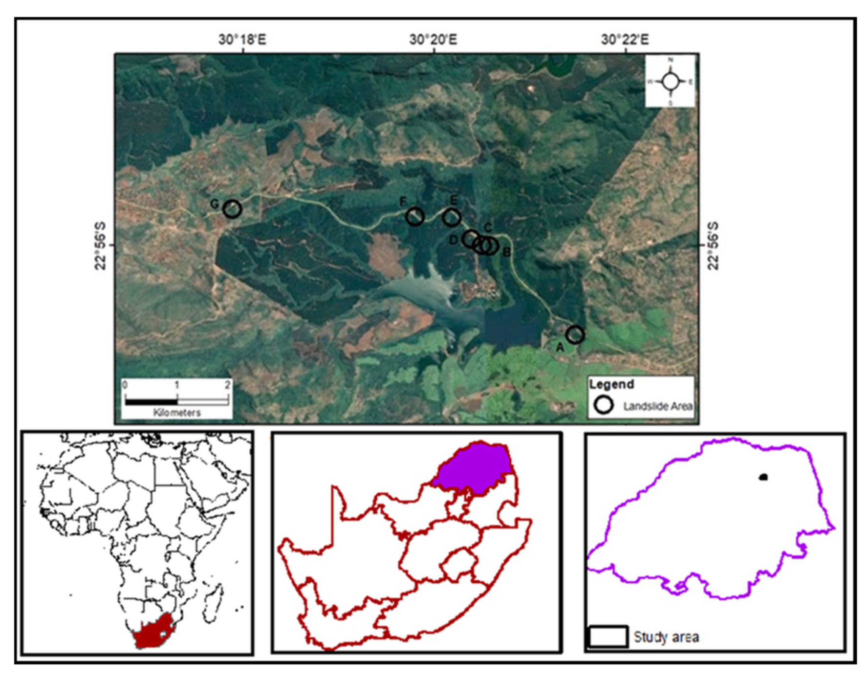
1.1. Locality of the Study Area
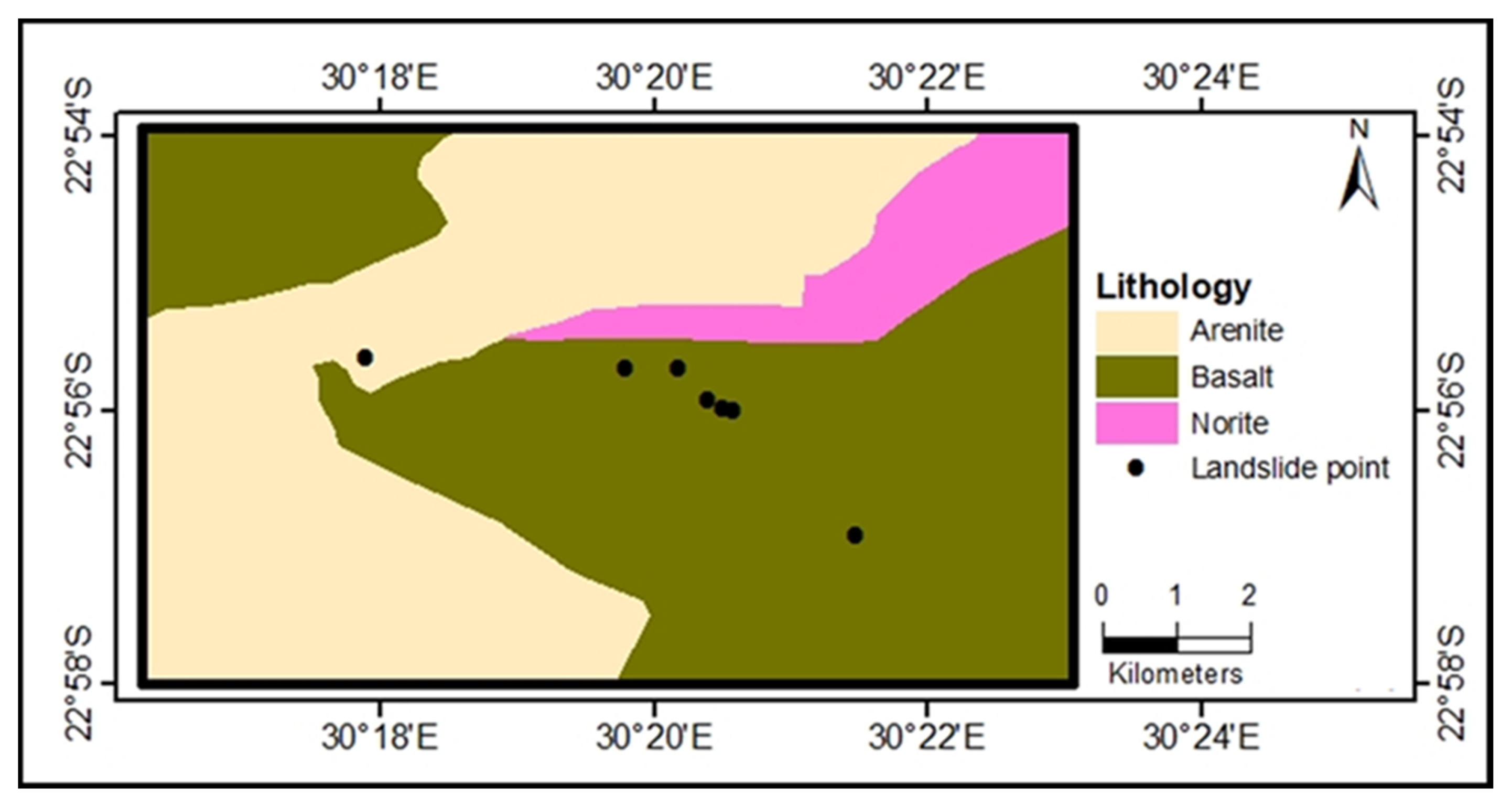
1.2. Geological Setting of the Study Area
2. Materials and Methods
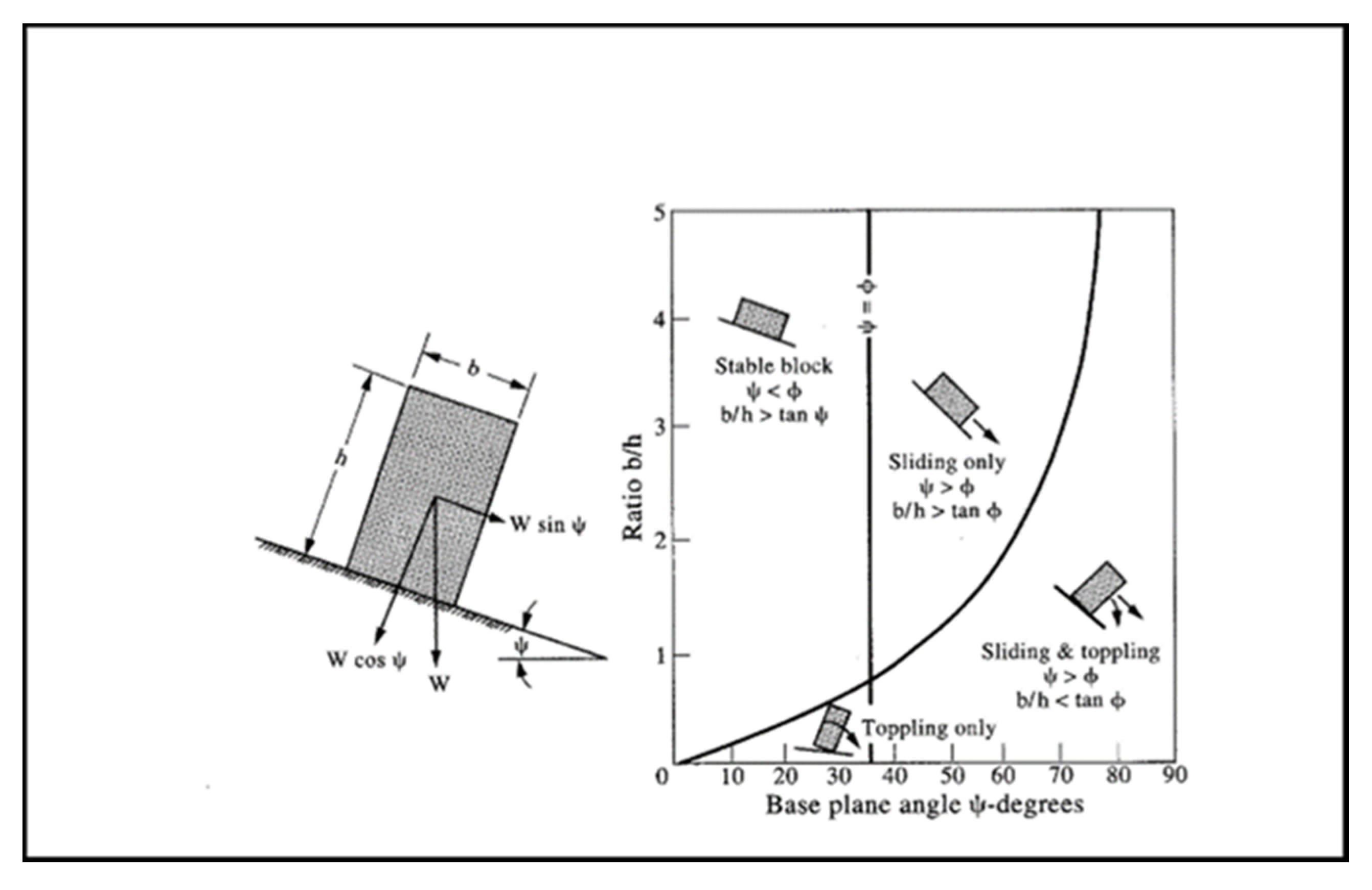
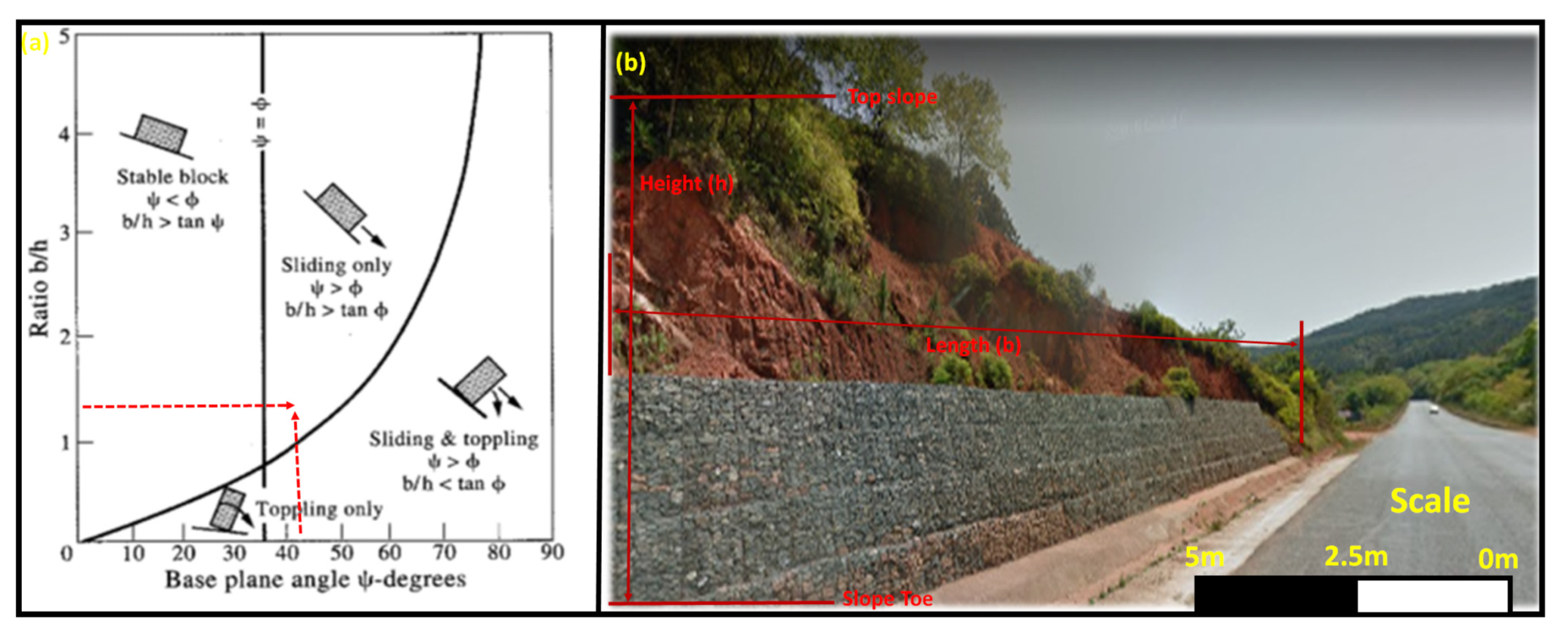
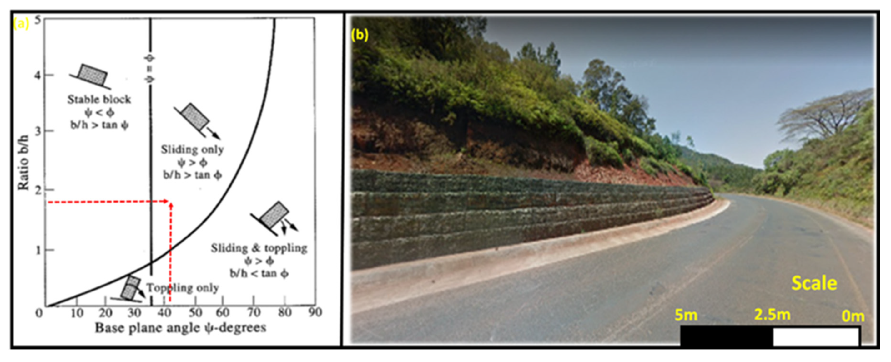
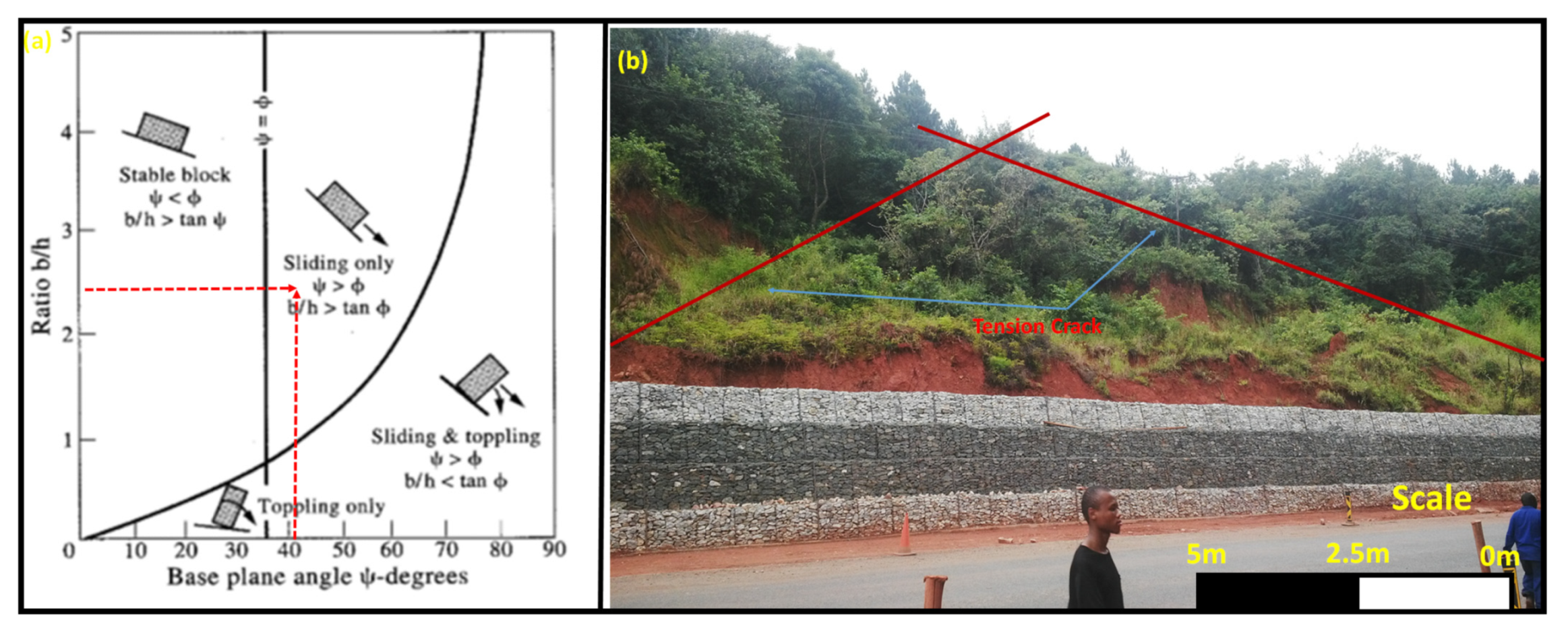
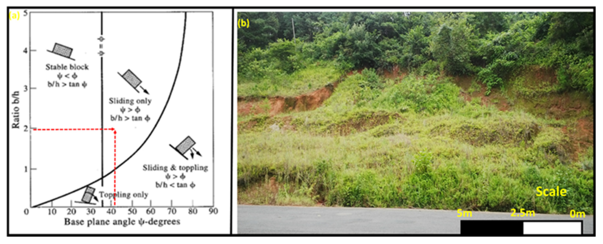
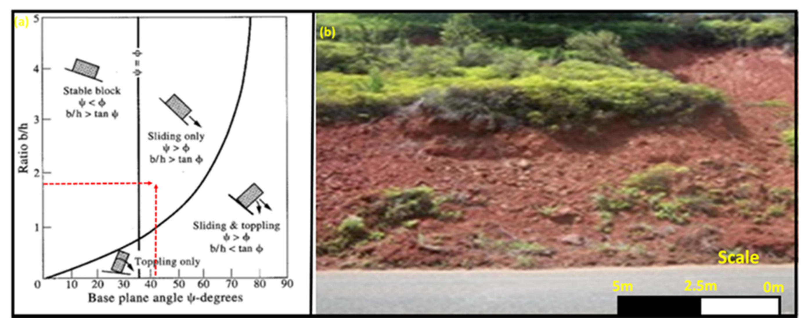
2.1. Toppling Analysis
2.2. Rotational Analysis
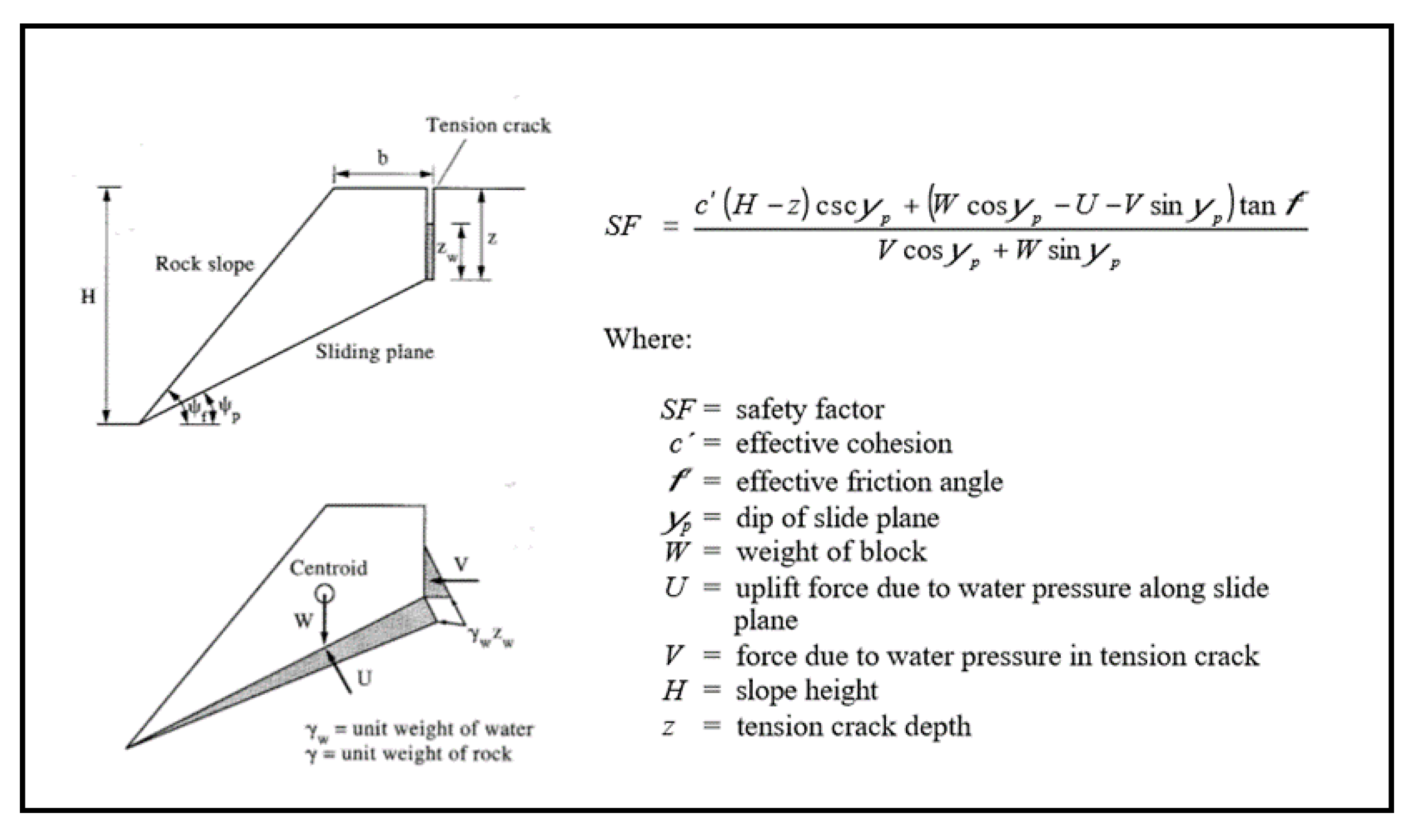
2.3. Transitional Analysis
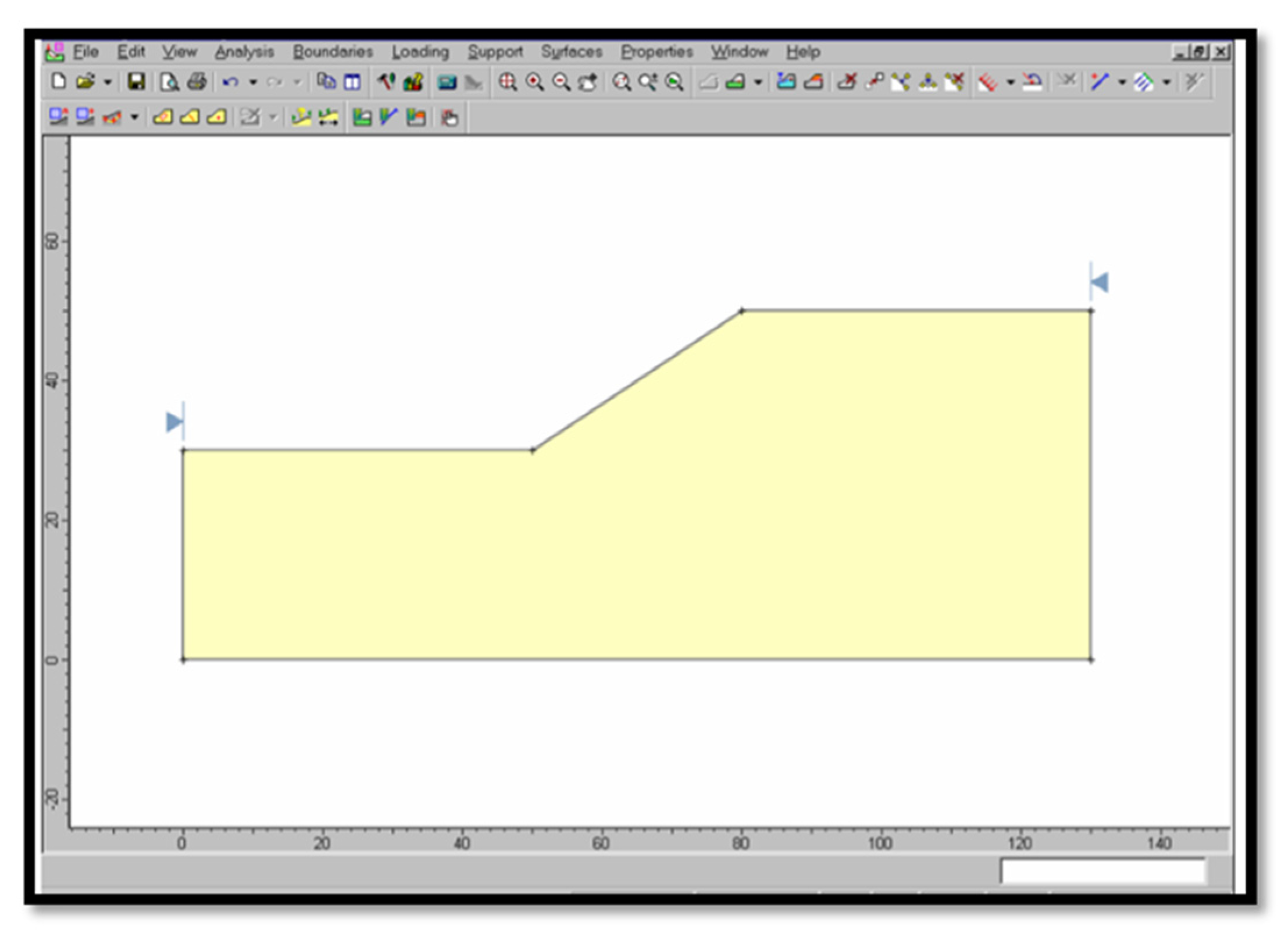
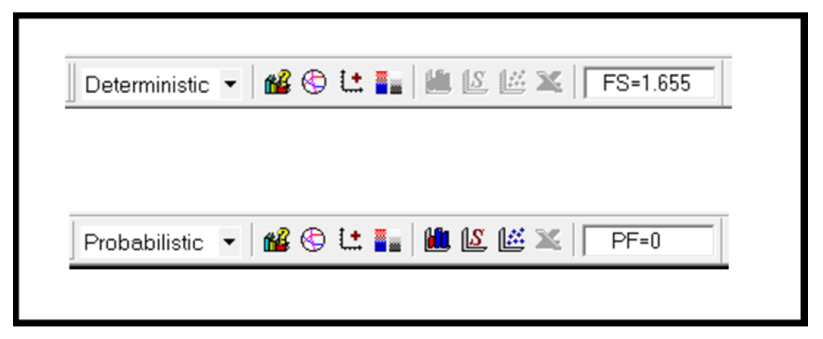
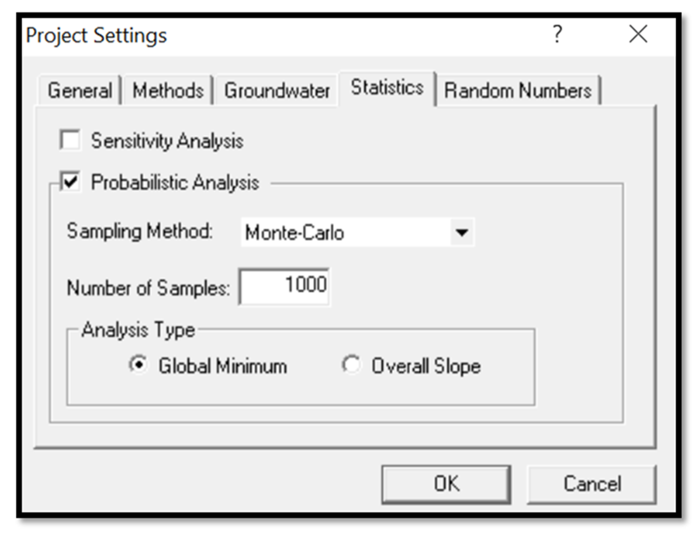
2.4. Numerical Simulation Procedures for SLIDES
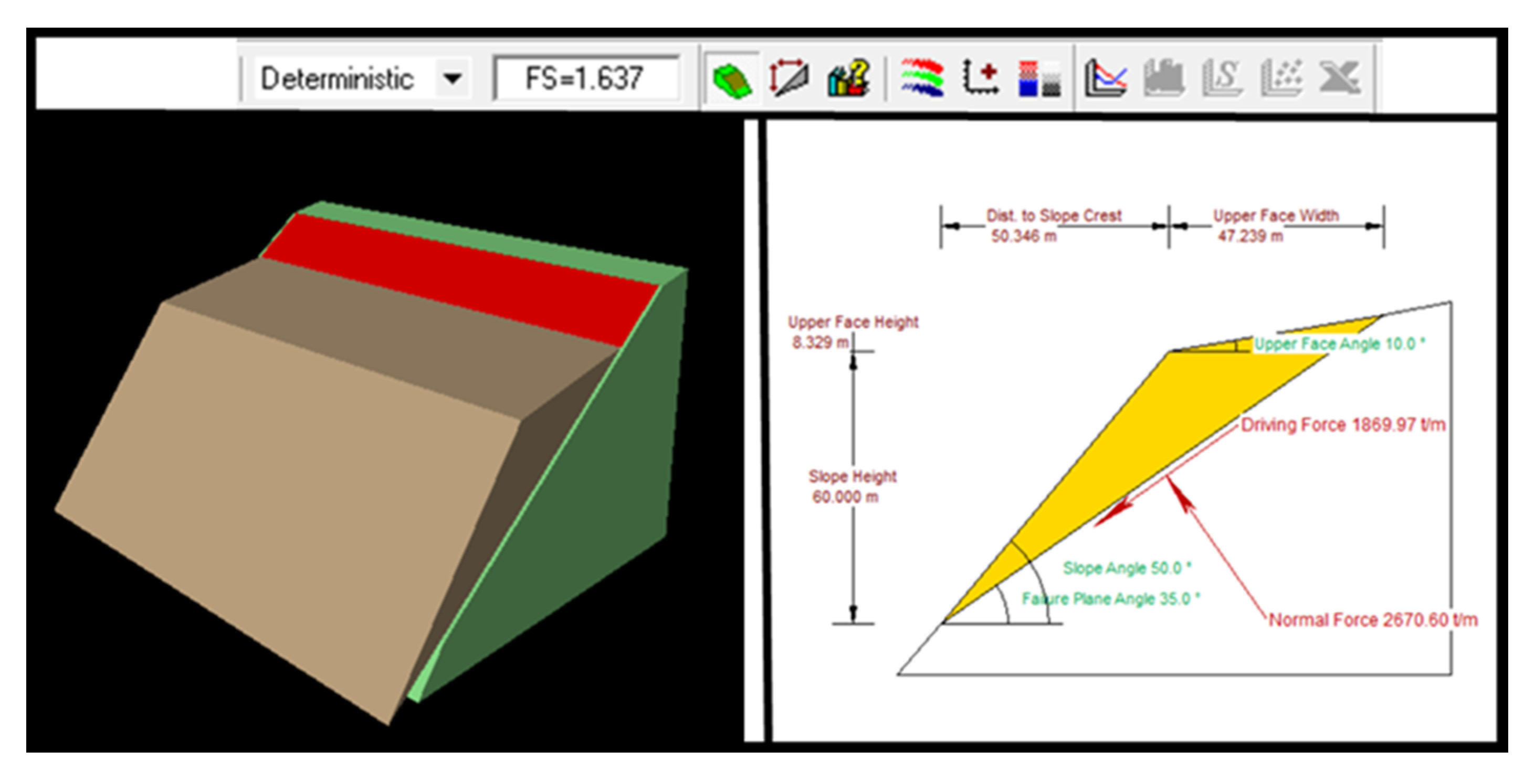
2.5. Numerical Simulation Procedures for RocPlane
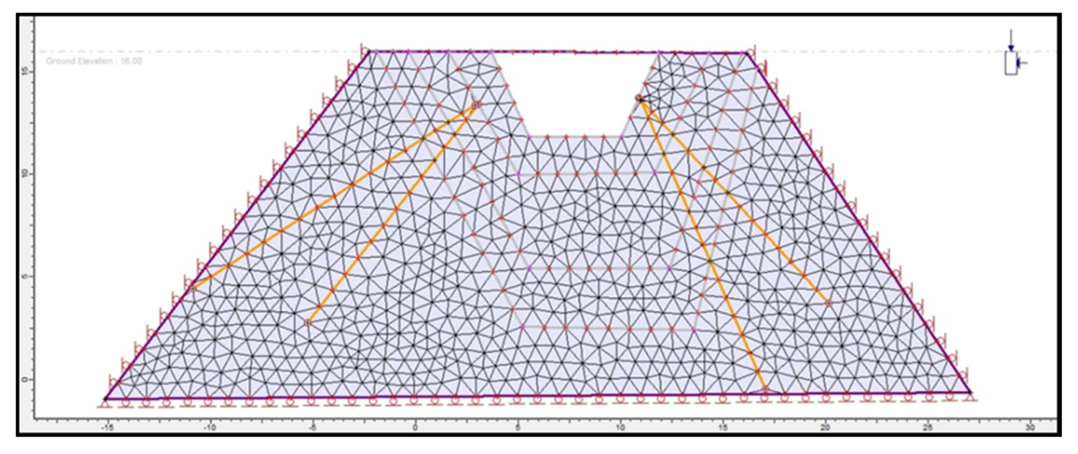
2.6. Numerical Simulation of Slope Stability Using Phase 2
3. Results and Discussions
3.1. Toppling Analysis
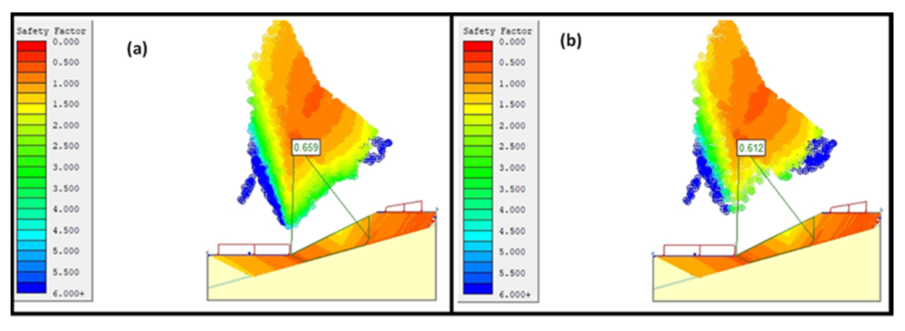
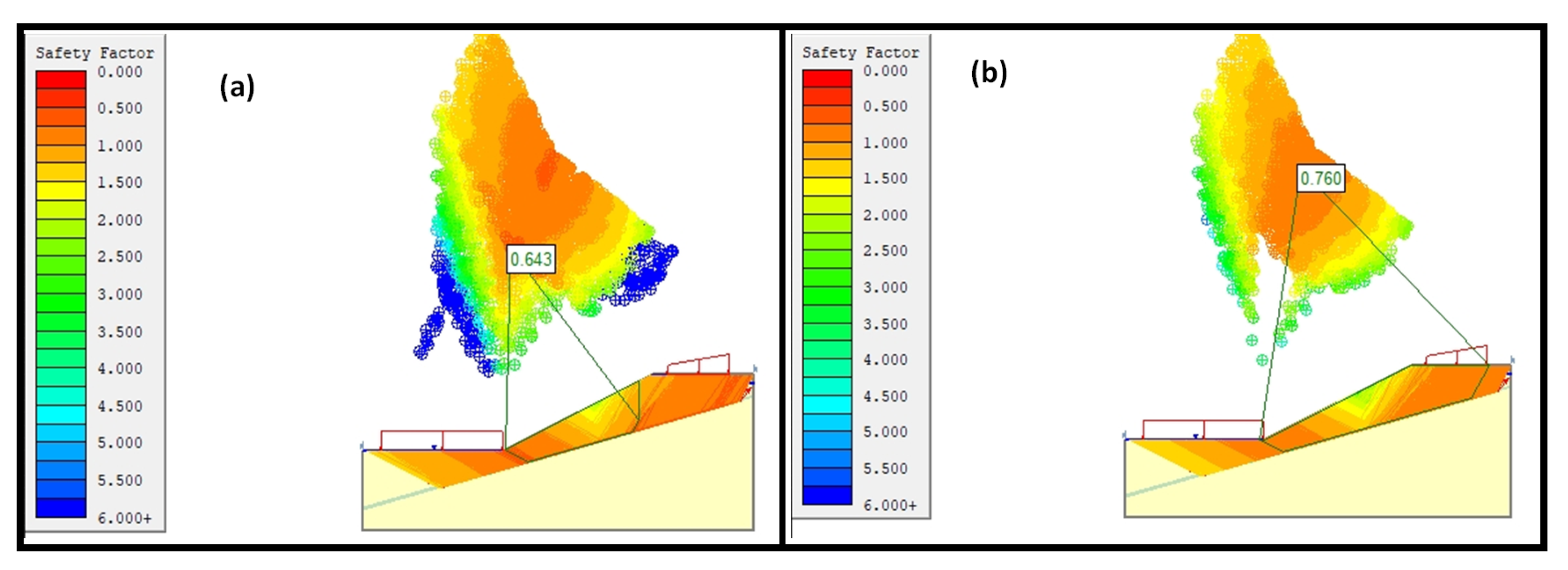
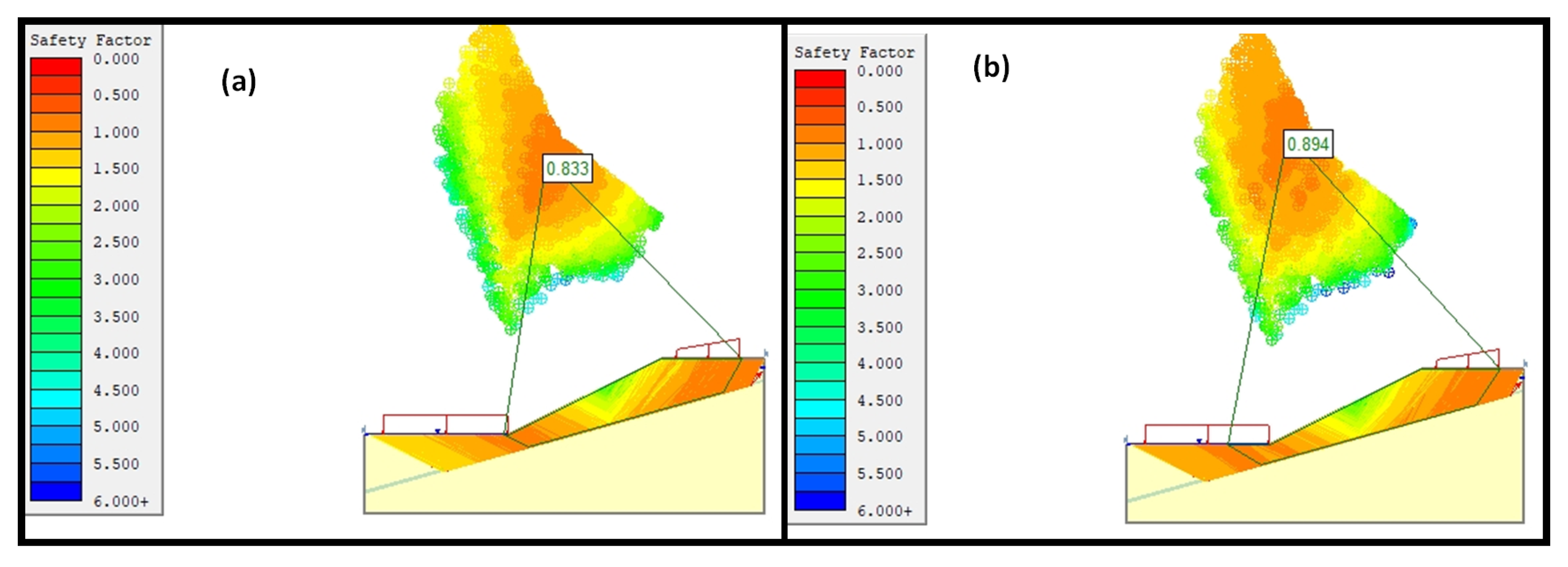
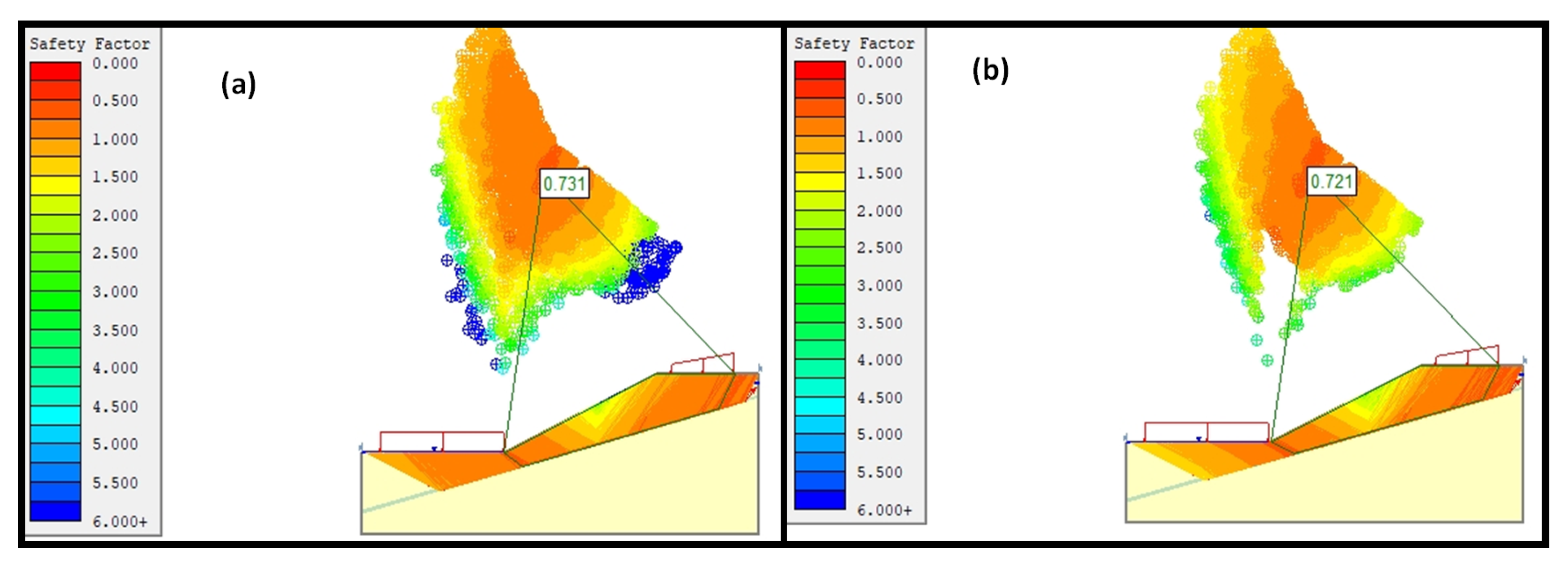
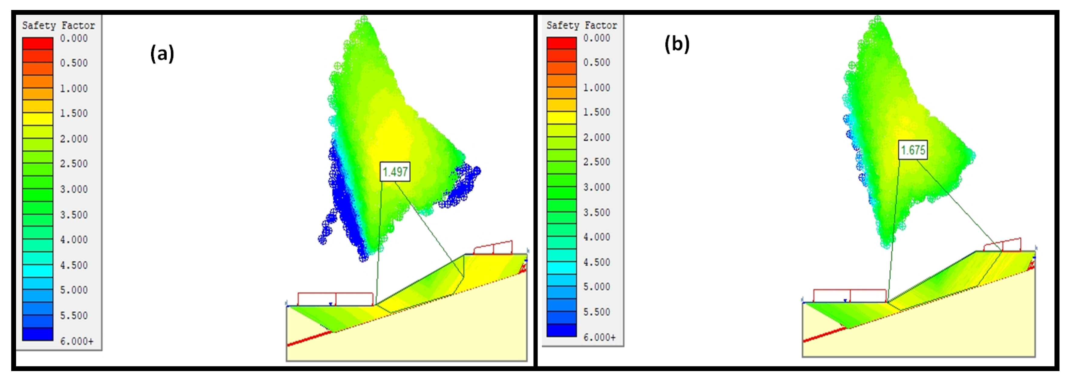
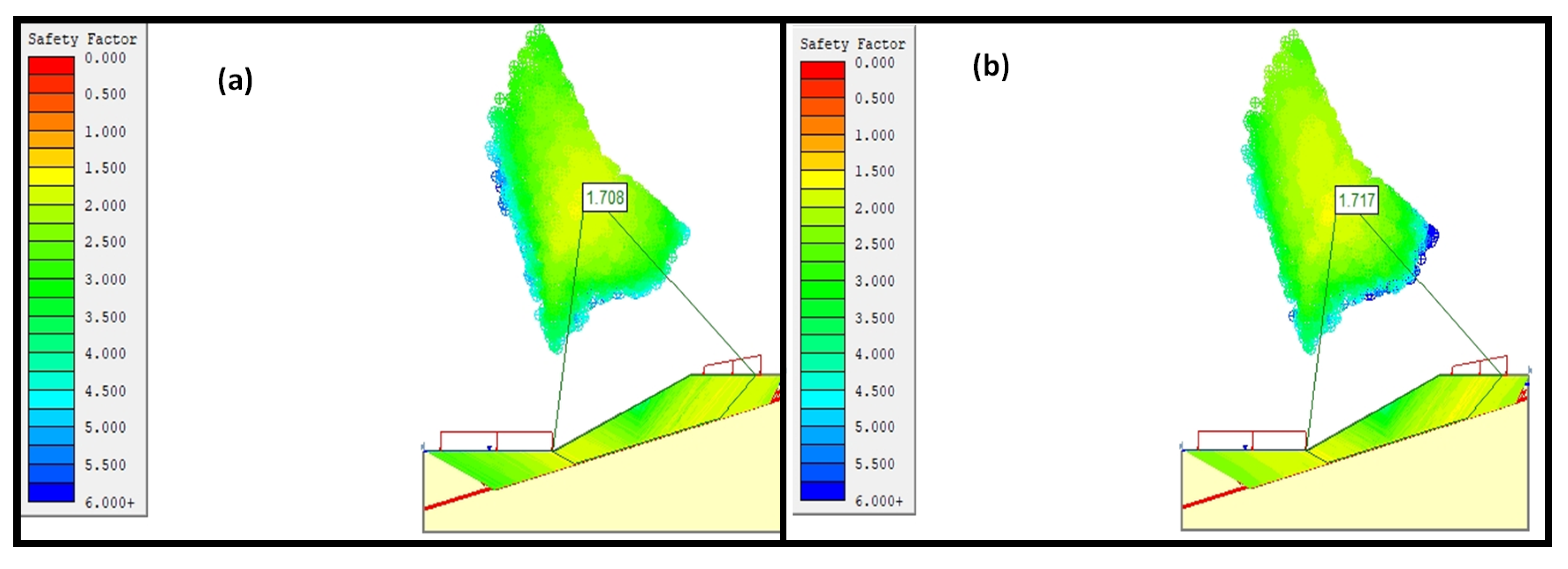
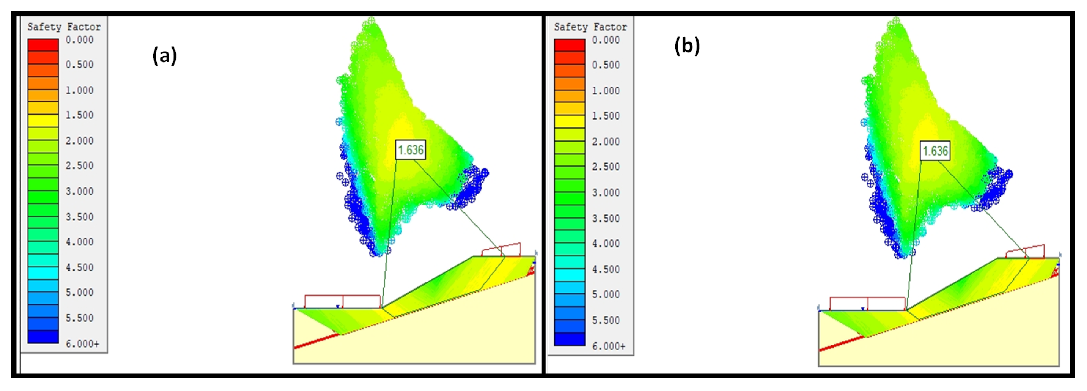
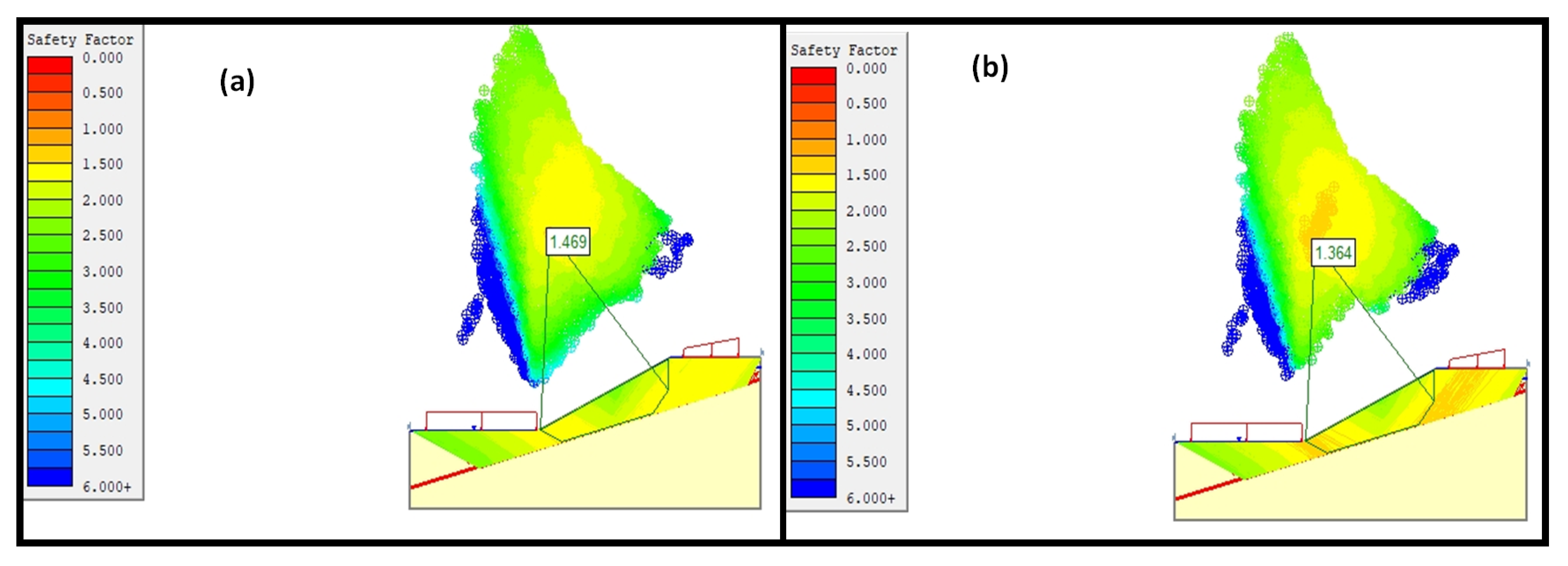
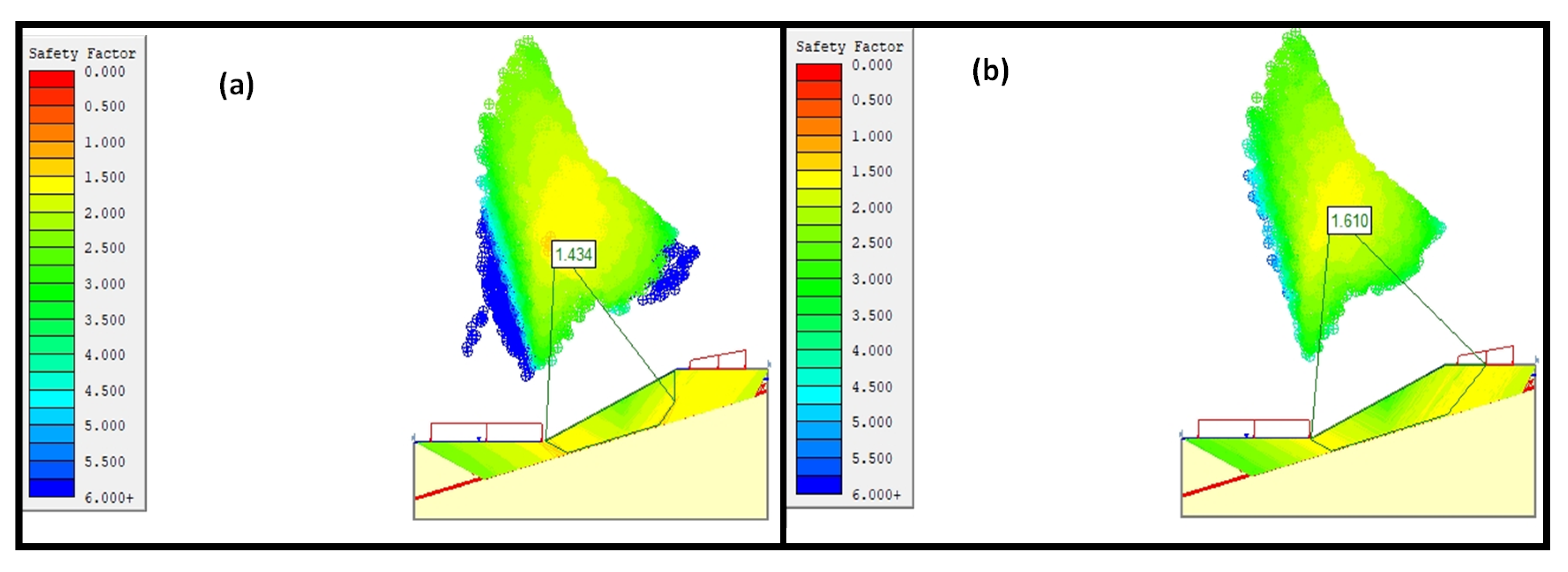
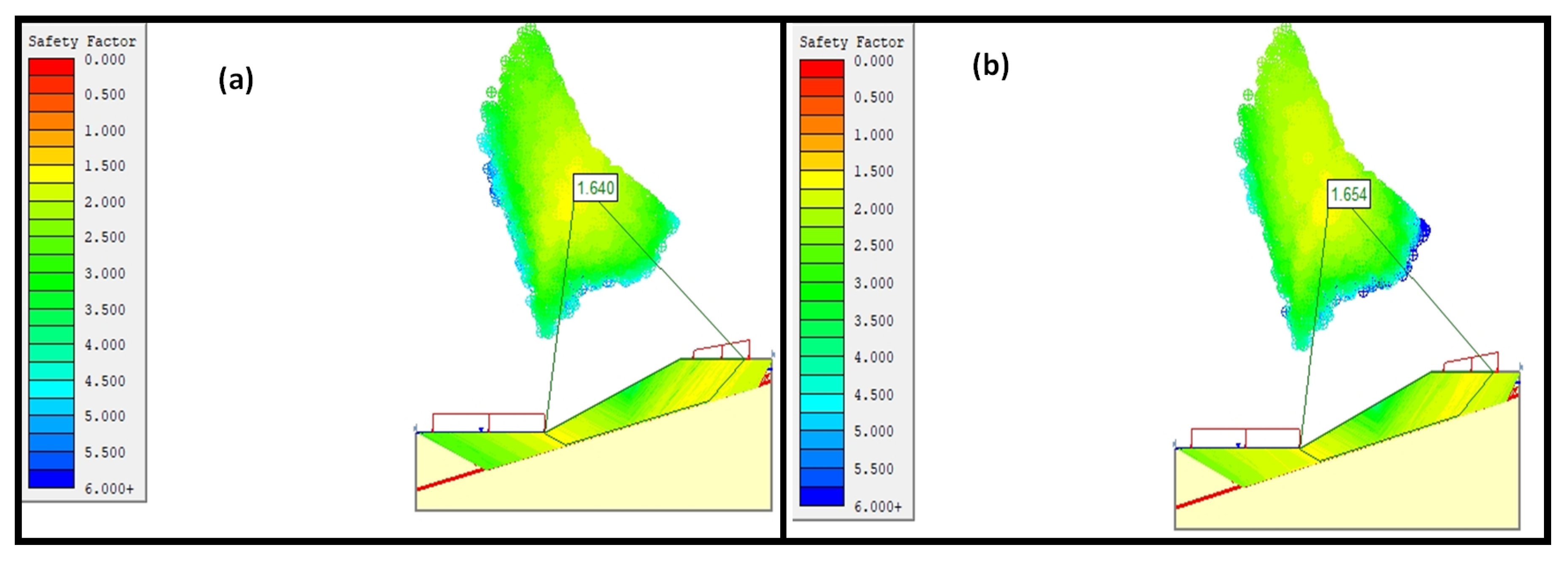
3.2. Rotational Analysis
3.3. Transitional Analysis
3.4. Advanced Numerical Simulation of Slope Stability
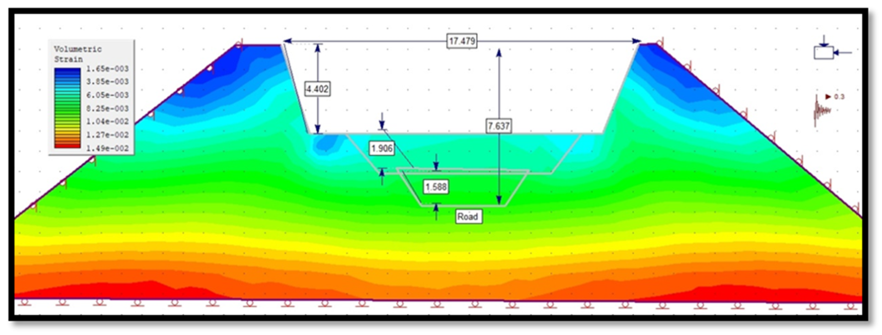
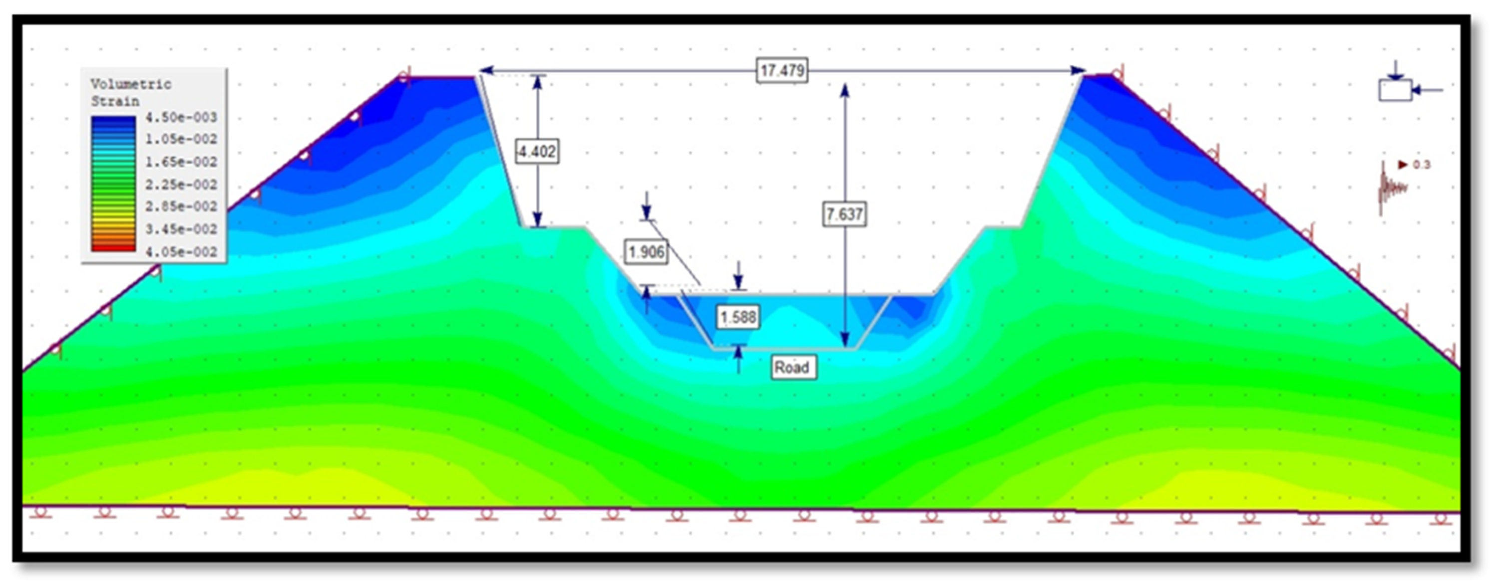
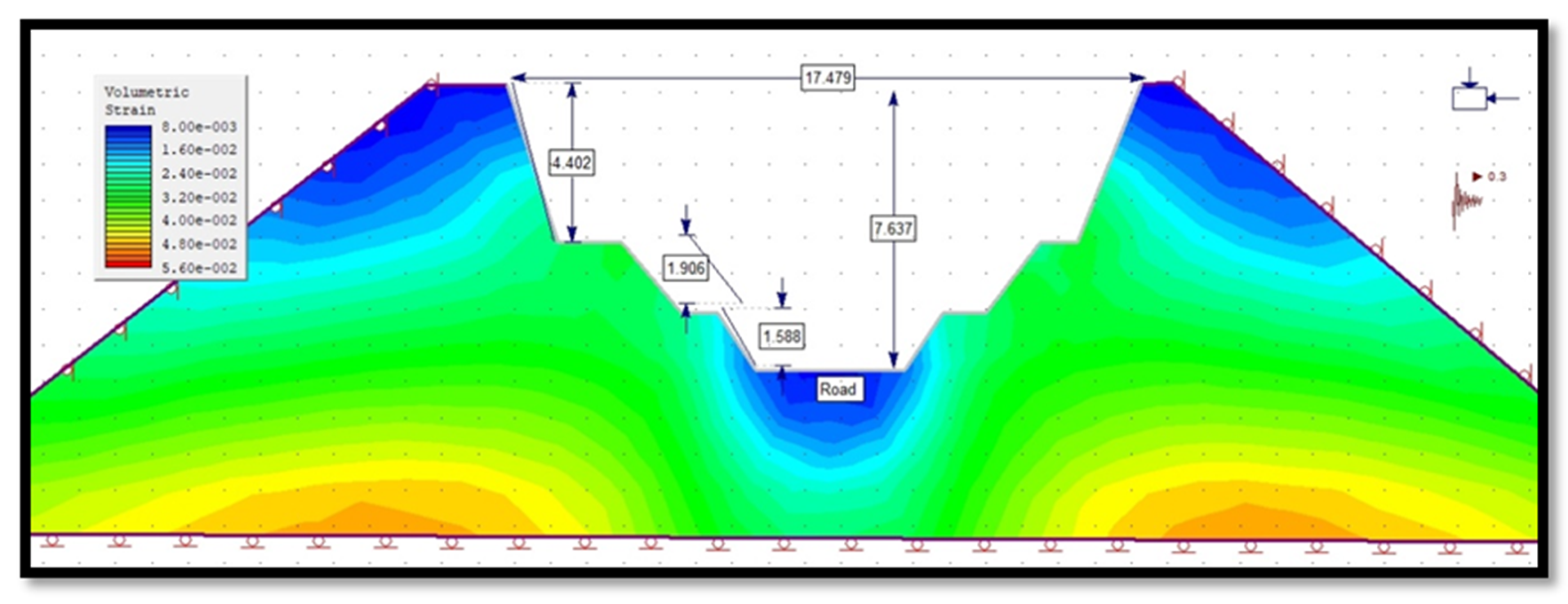
3.4.1. Volumetric Strain of Slope in Phase 2
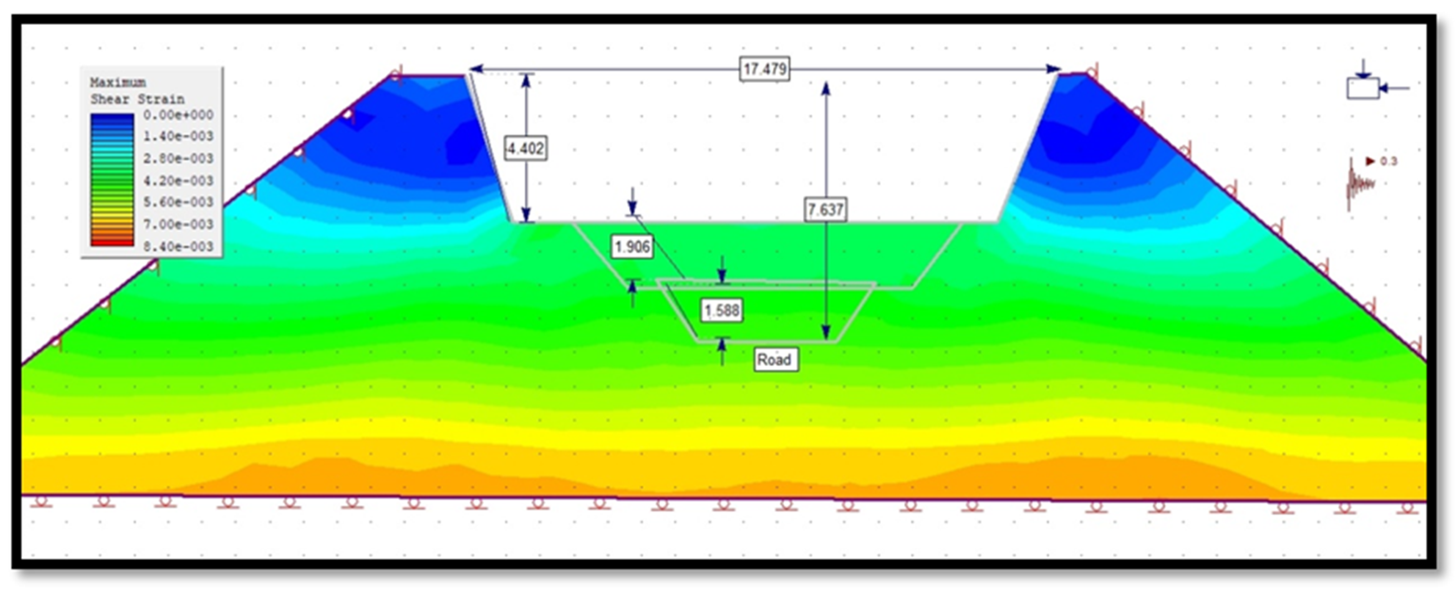
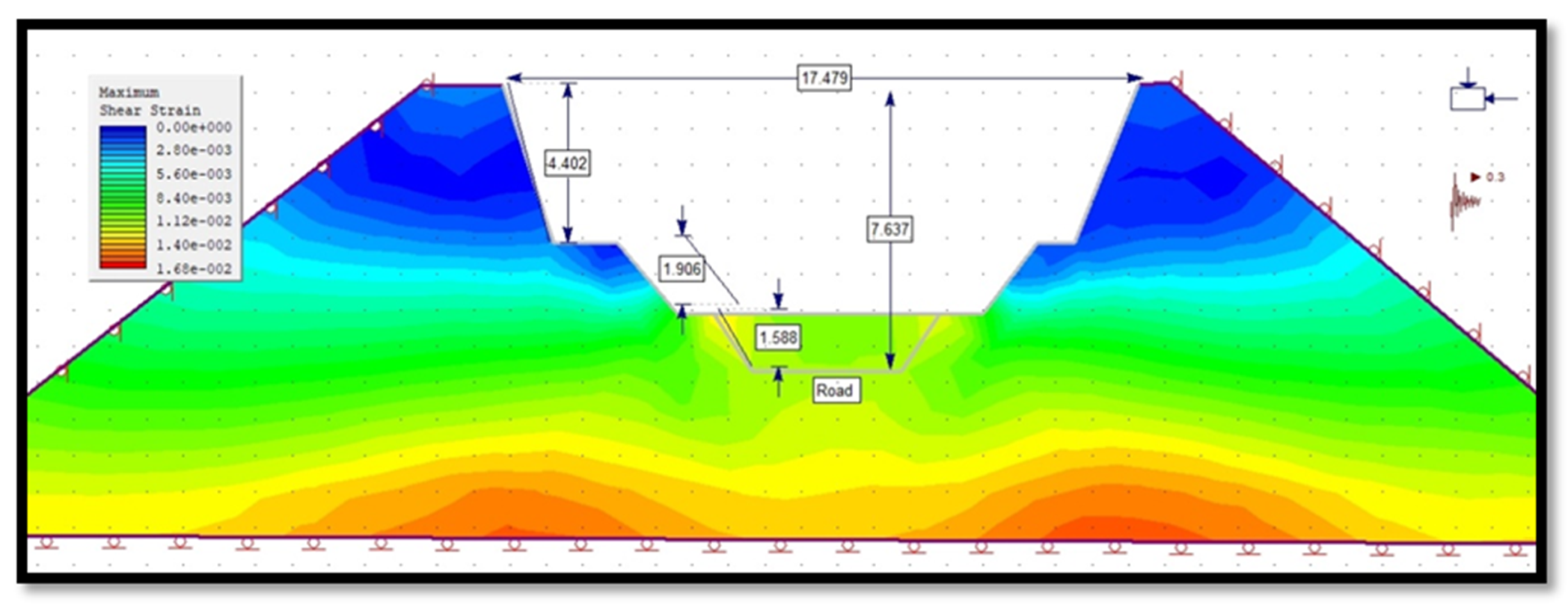
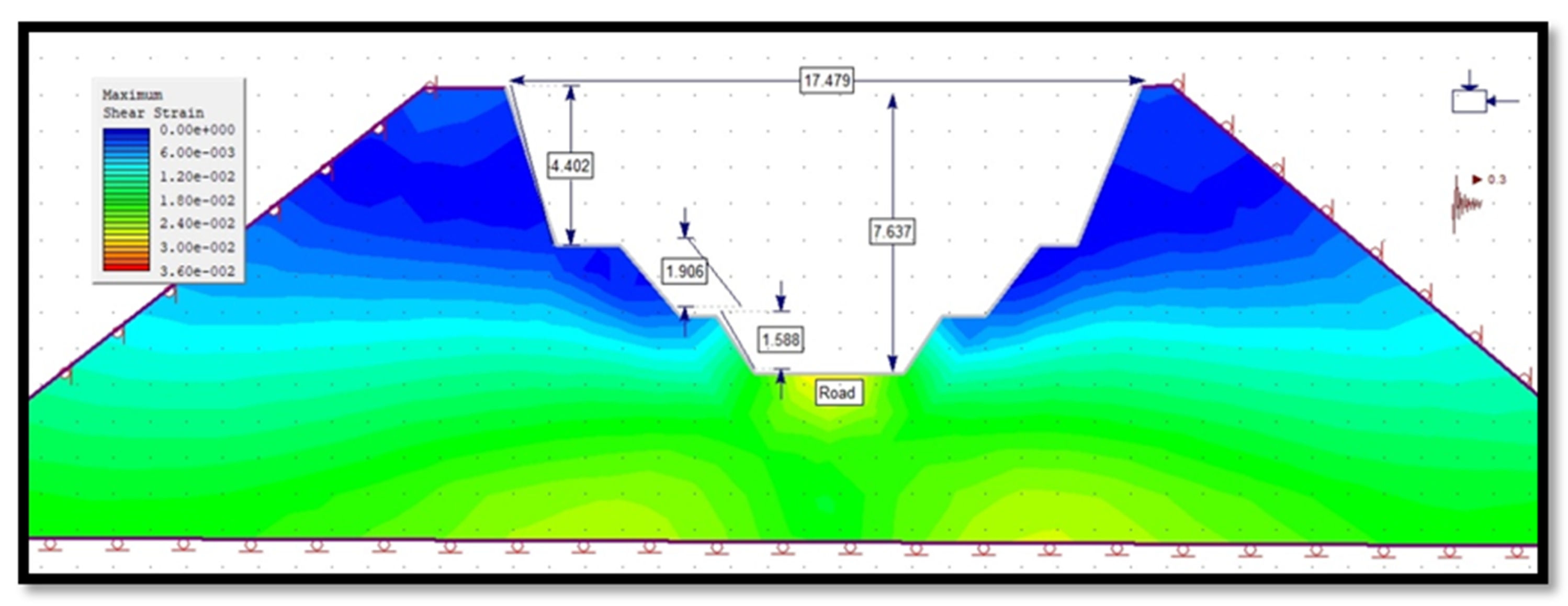
3.4.2. Maximum Shear Strain of Slope in Phase 2
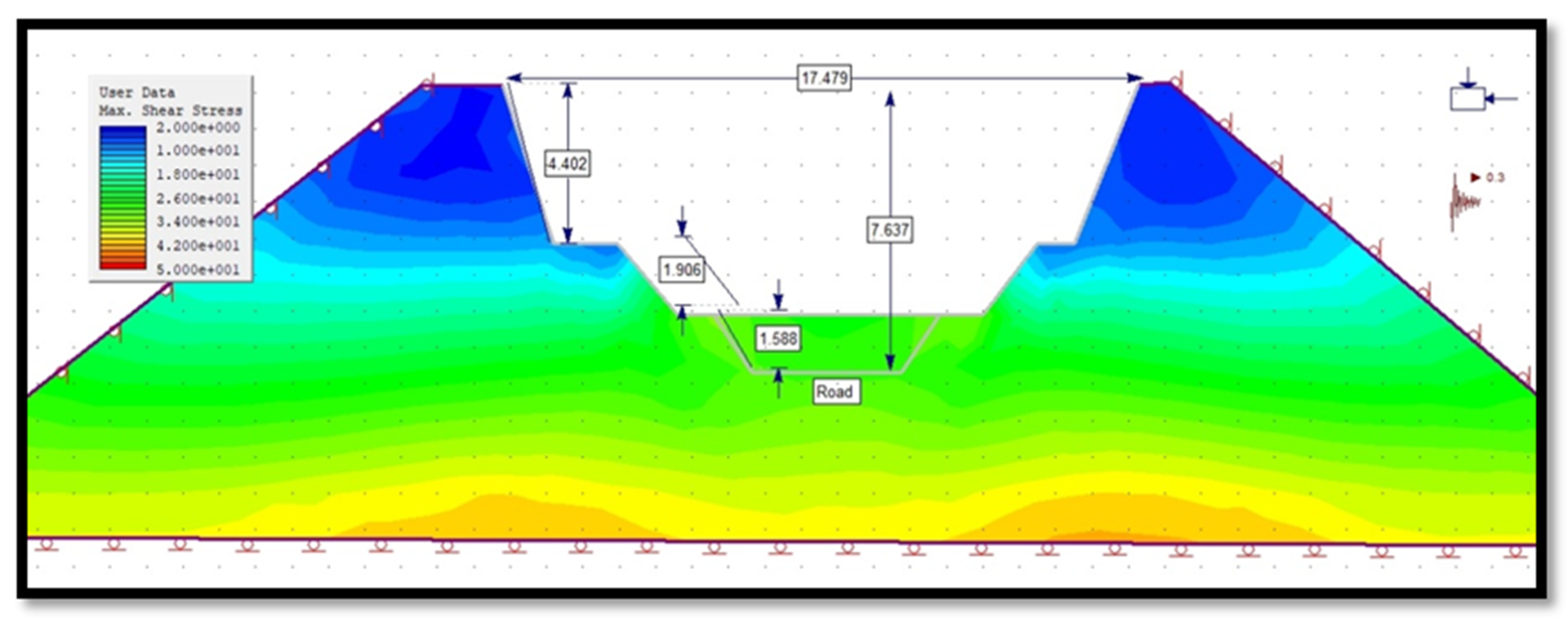
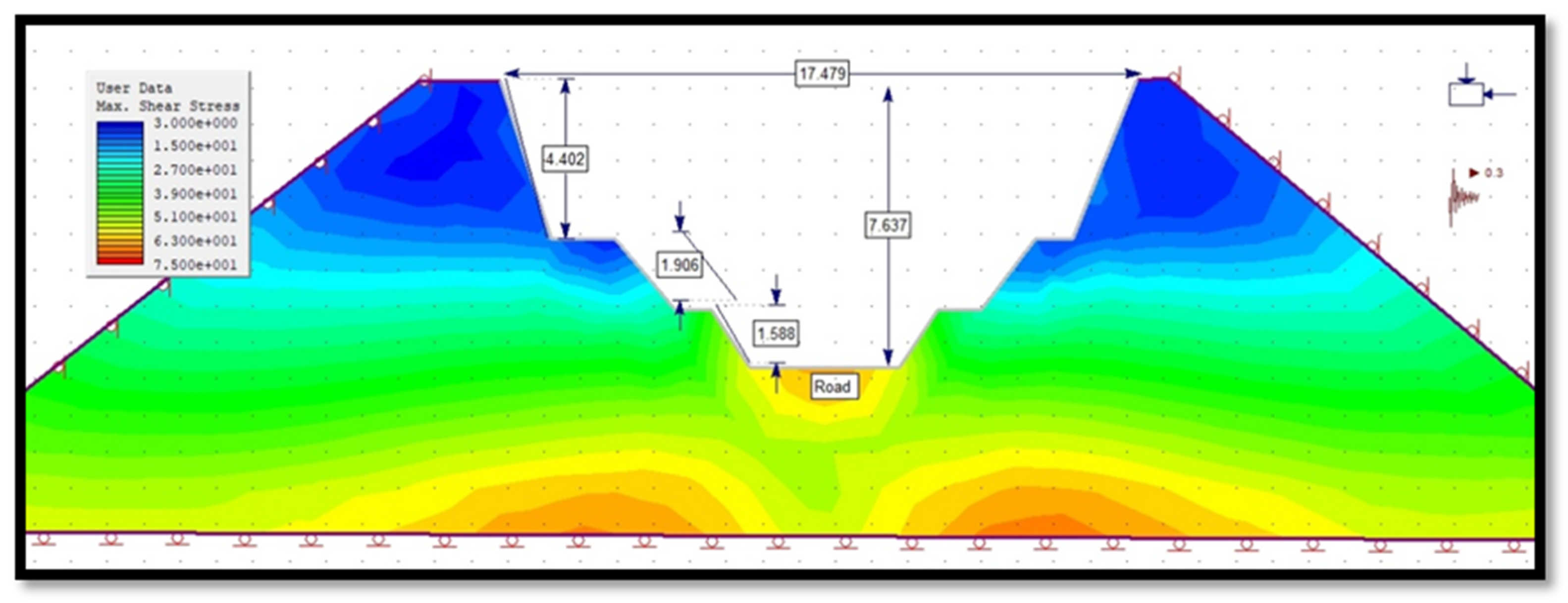
3.4.3. Maximum Shear Stress of Slope in Phase 2
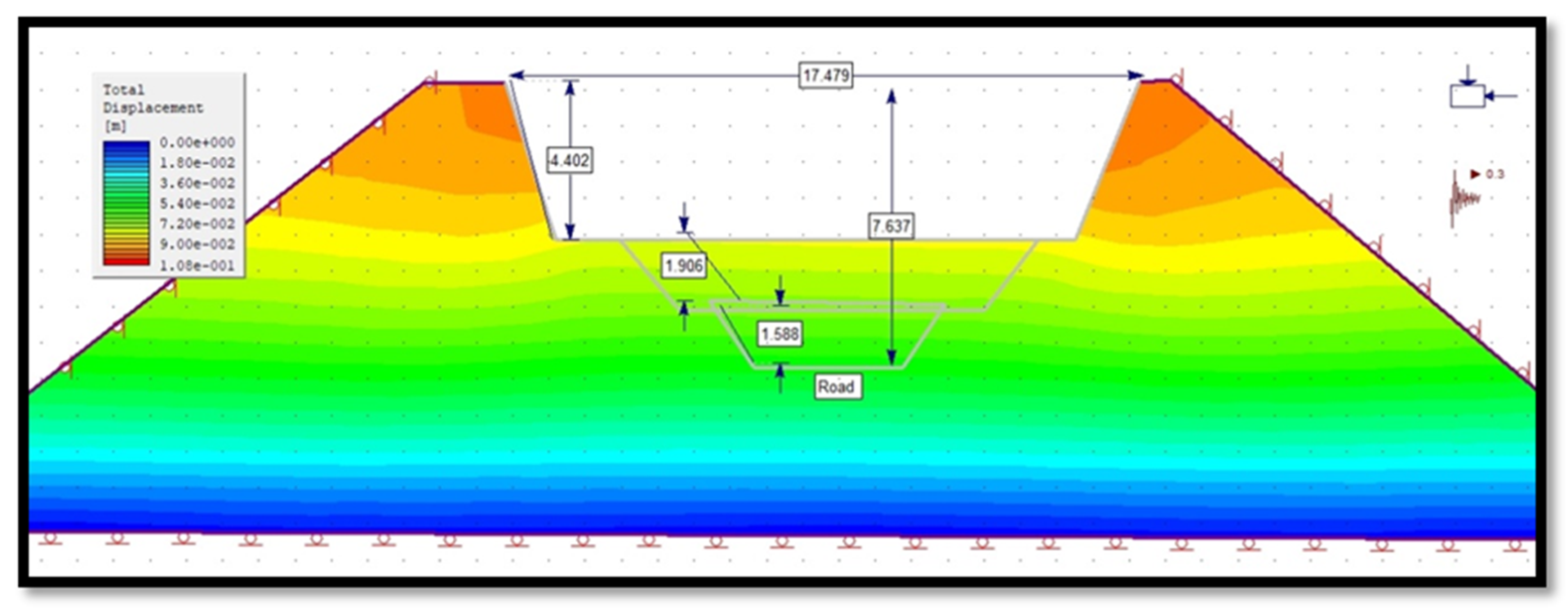
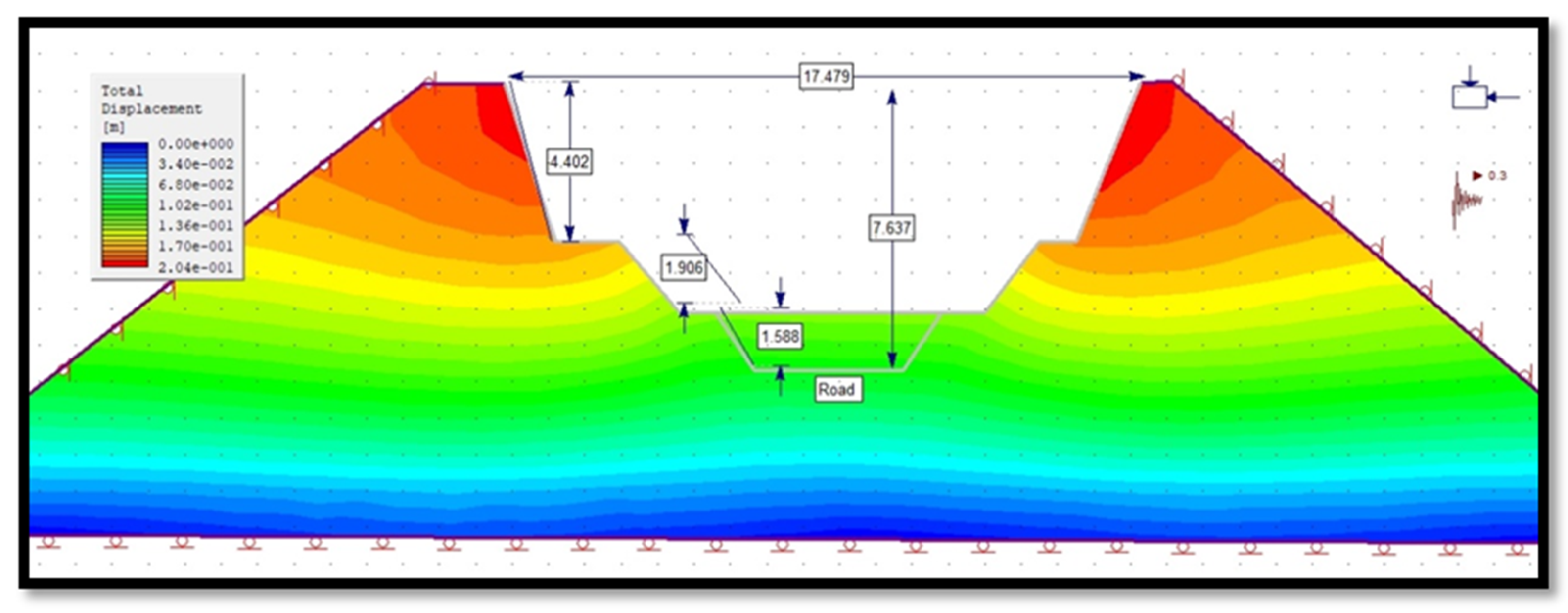
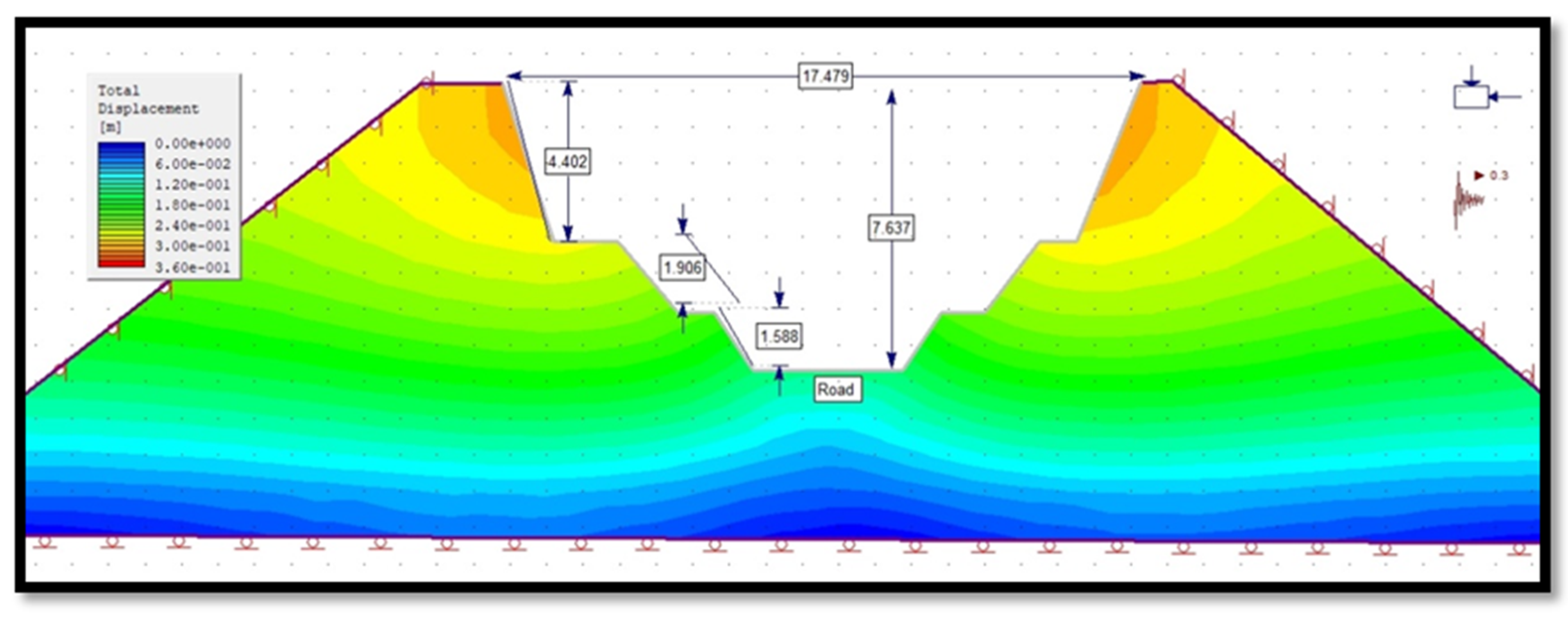
3.4.4. Total Displacement of Slope in Phase 2
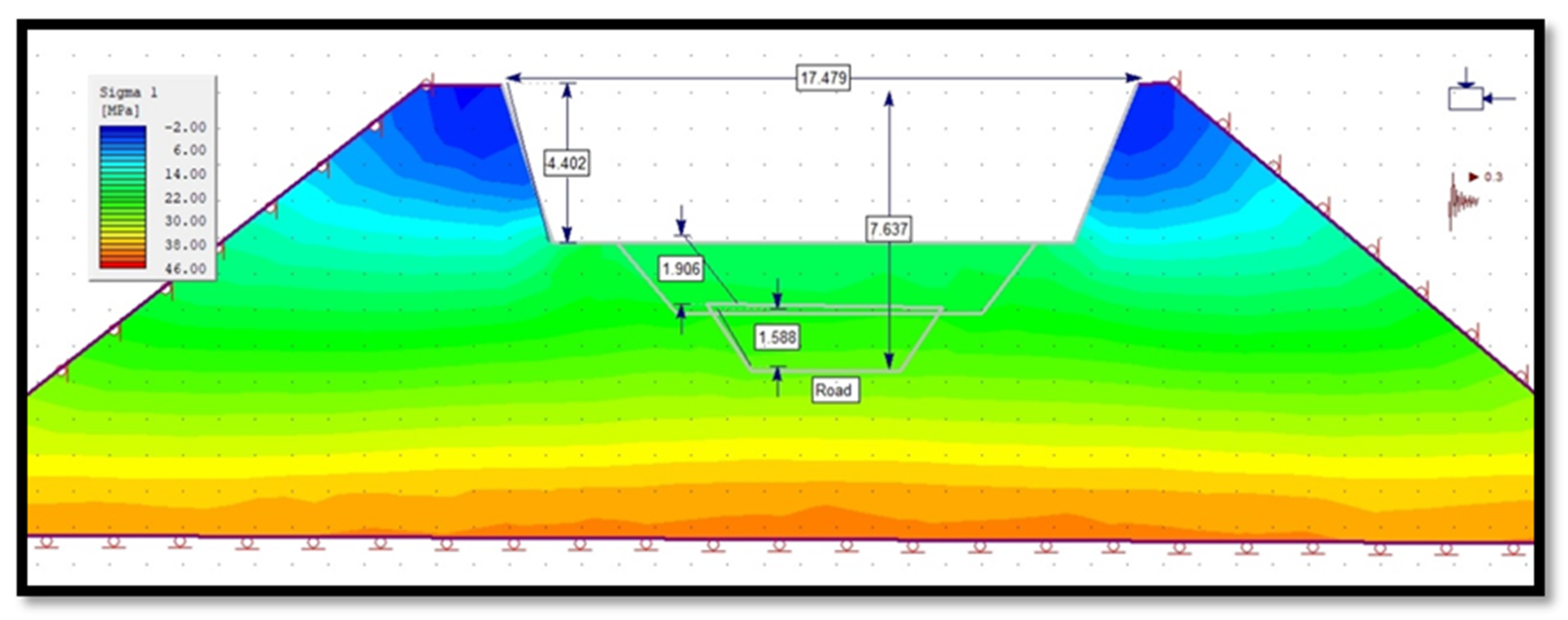
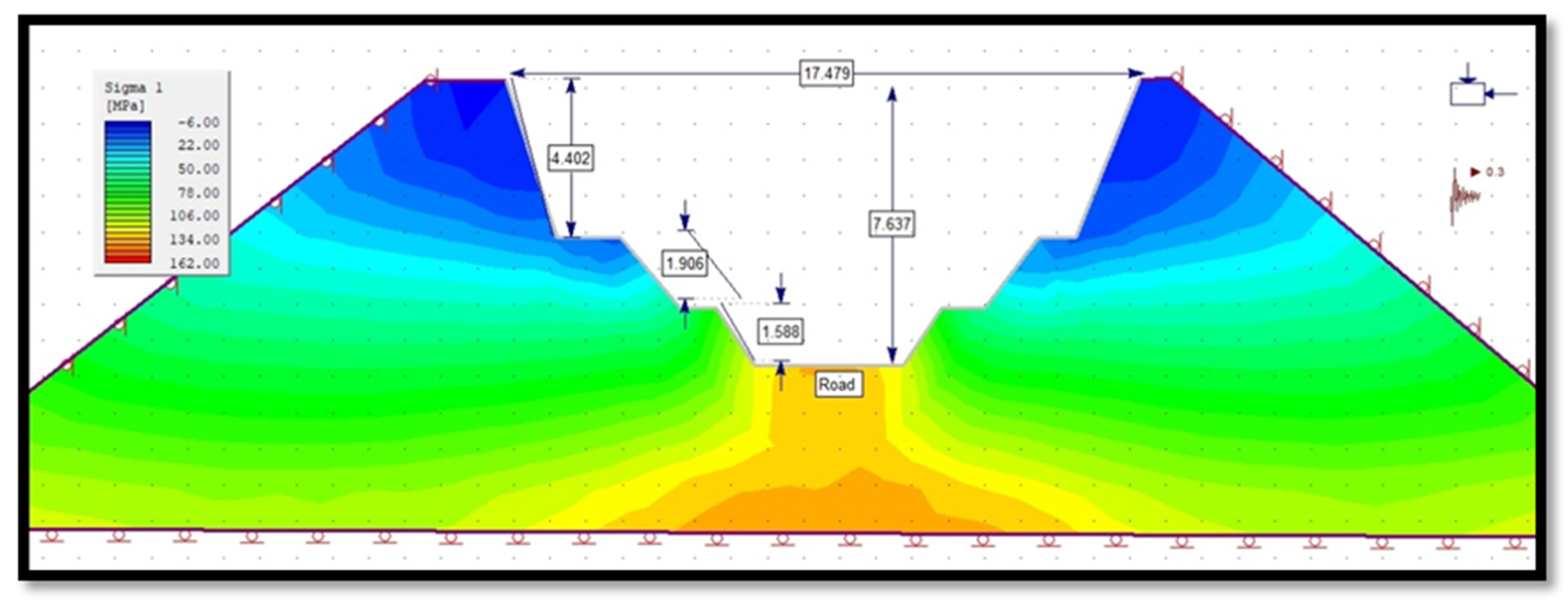
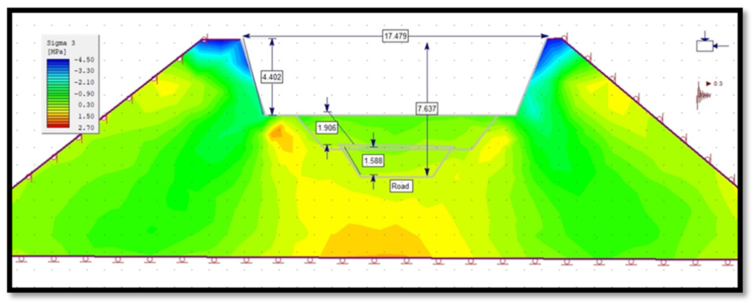
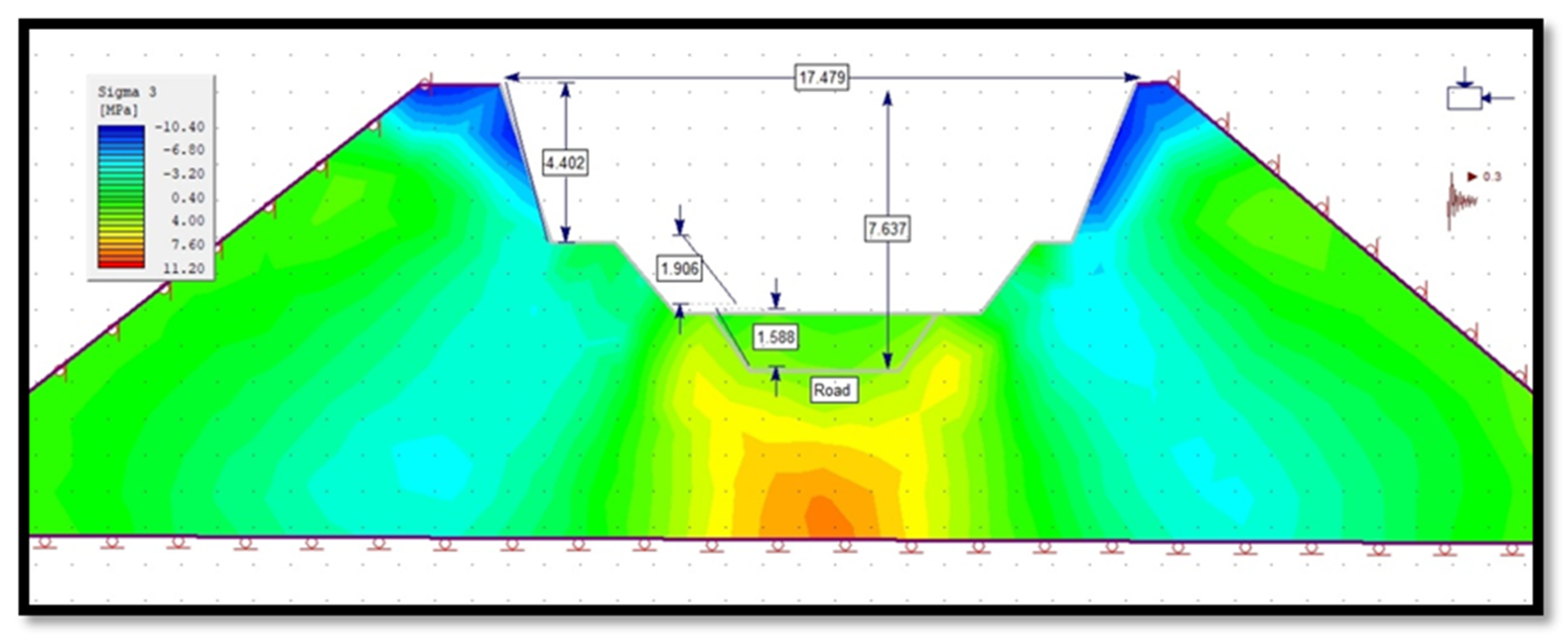
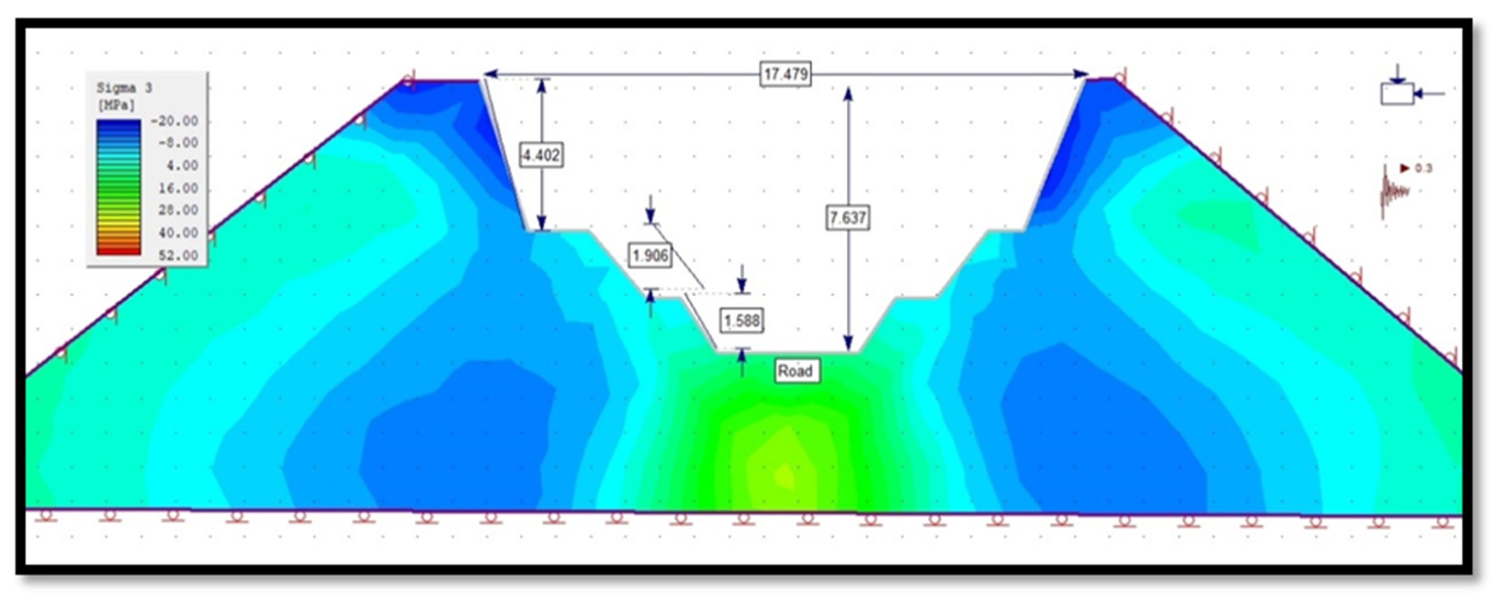
3.4.5. Principal Stress of Slope in Phase 2
4. Conclusions
Author Contributions
Funding
Acknowledgments
Conflicts of Interest
References
- Dilley, M. Natural Disaster Hotspots: A Global Risk Analysis; The World Bank: Washington, DC, USA, 2005. [Google Scholar]
- Gariano, S.L.; Guzzetti, F. Landslides in a changing climate. Earth-Sci. Rev. 2016, 162, 227–252. [Google Scholar] [CrossRef]
- Haque, U.; Blum, P.; da Silva, P.F.; Andersen, P.; Pilz, J.; Chalov, S.R.; Malet, J.P.; Auflic, M.J.; Andres, N.; Poyiadji, E.; et al. Fatal landslides in Europe. Landslides 2016, 1545–1554. [Google Scholar] [CrossRef]
- Kjekstad, O.; Highland, L. Economic and Social Impacts of Landslides. In Landslides-Disaster RiskReduction; Springer: Berlin/Heidelberg, Germany, 2009; pp. 573–587. [Google Scholar] [CrossRef]
- Petley, D. Global patterns of loss of life from landslides. Geology 2012, 40, 927–930. [Google Scholar] [CrossRef]
- Landslides-Disaster Risk Reduction; Sassa, K., Canuti, P., Eds.; Springer: Berlin/Heidelberg, Germany, 2009. [Google Scholar]
- Stanley, T.; Kirschbaum, D.B. A heuristic approach to global landslide susceptibility mapping. Nat. Hazards 2017. [Google Scholar] [CrossRef]
- Kirschbaum, D.; Stanley, T.; Zhou, Y. Spatial and temporal analysis of a global landslide catalog. Geomorphology 2015, 249, 4–15. [Google Scholar] [CrossRef]
- Kirschbaum, D.B.; Adler, R.; Hong, Y.; Hill, S.; Lerner-Lam, A. A global landslide catalog for hazard applications: Method, results, and limitations. Nat. Hazards 2010, 52, 561–575. [Google Scholar] [CrossRef]
- Maes, J.; Kervyn, M.; de Hontheim, A.; Dewitte, O.; Jacobs, L.; Mertens, K.; Vanmaercke, M.; Vranken, L.; Poesen, J. Landslide risk reduction measures: A review of practices and challenges for the tropics. Prog. Phys. Geogr. 2017, 41, 191–221. [Google Scholar] [CrossRef]
- Nadim, F.; Kjekstad, O.; Peduzzi, P.; Herold, C.; Jaedicke, C. Global landslide and avalanche hotspots. Landslides 2006, 3, 159–173. [Google Scholar] [CrossRef]
- Reichenbach, P.; Rossi, M.; Malamud, B.; Mihir, M.; Guzzetti, F. A Review of Statistically-Based Landslide Susceptibility Models. Earth Sci. Rev. 2018, 180, 60–91. [Google Scholar] [CrossRef]
- Hong, Y.; Adler, R.; Huffman, G. Use of satellite remote sensing data in the mapping of global landslide susceptibility. Nat. Hazards 2007, 43, 245–256. [Google Scholar] [CrossRef]
- Kirschbaum, D.B.; Adler, R.; Hong, Y.; Lerner-Lam, A. Evaluation of a preliminary satellite-based landslide hazard algorithm using global landslide inventories. Nat. Hazards Earth Syst. Sci. 2009, 9, 673–686. [Google Scholar] [CrossRef]
- Gerland, P.; Raftery, A.E.; Ev Ikova, H.; Li, N.; Gu, D.; Spoorenberg, T.; Alkema, L.; Fosdick, B.K.; Chunn, J.; Lalic, N.; et al. World population stabilization unlikely this century. Science 2014, 346, 234–237. [Google Scholar] [CrossRef] [PubMed]
- Thulamela Municipality. Background of Thulamela Municipality. Thulamela Municipality Limpopo Province; 2019. Available online: http://www.thulamela.gov.za/ (accessed on 30 March 2019).
- Barker, O.B. A Contribution to the Geology of the Soutpansberg Group, Waterberg Supergroup, Northern Transvaal. Ph.D. Thesis, University of the Witwatersrand, Johannesburg, South Africa, 1979. [Google Scholar]
- Barker, O.B.; Brandl, G.; Callaghan, C.C.; Erikson, P.G.; van der Neut, M. The Soutpansberg and Waterburg Groups and the Blouberg formation. In The Geology of South Africa; Anhaeusser, M.R., Thomas, C.R., Johnson, R.J., Eds.; Council for Geosciences, Geological Society of South Africa: Pretoria, South Africa, 2006; pp. 301–324. [Google Scholar]
- Brandl, G. The Geology of the Messina Area, Explain, Sheet 2230 (Messina); Geology Survey of South Africa: Pretoria, South Africa, 1981; Report number 35. [Google Scholar]
- Brandl, G. The Geology of Pieterburg Area, Explain, Sheet 2230 (Pietersburg); Geology Survey of South Africa: Pretoria, South Africa, 1986; Report number 43. [Google Scholar]
- Sengani, F.; Zvarivadza, T. Evaluation of Factors Influencing Slope Instability: Case Study of the R523 Road between Thathe Vondo and Khalavha Area in South Africa; Symposium of Environmental Issues and Waste Management in Energy and Mineral Production; Springer: Cham, Switzerland, 2019; pp. 81–89. [Google Scholar]
- Mutanamba, M. Analyze the Stability of Cut Slopes along the R523 Road between Thathe Vondo and Khalavha Area and to Find the Most Appropriate Stabilization Methods to Prevent Future Slope Failure along the Road R523. Master’s Thesis, University of Venda, Thohoyandou, South Africa, 2013. [Google Scholar]
- Abolmasov, B.; Milenković, S.; Marjanović, M.; Durić, U.; Jelisavac, B. A geotechnical model of the Umka landslide with reference to landslides in weathered Neogene marls in Serbia. Landslides 2015, 12, 689–702. [Google Scholar] [CrossRef]
- Antronico, L.; Borrelli, L.; Coscarelli, R.; Gullà, G. Time evolution of landslide damages to buildings: The case study of Lungro (Calabria, Southern Italy). Bull. Eng. Geol. Environ. 2015, 74, 47–59. [Google Scholar] [CrossRef]
- Barla, G.; Antolini, F.; Barla, M.; Mensi, E.; Piovano, G. Monitoring of the Beauregard landslide (Aosta Valley, Italy) using advanced and conventional techniques. Eng. Geol. 2010, 116, 218–235. [Google Scholar] [CrossRef]
- Guzzetti, F.; Mondini, A.C.; Cardinali, M.; Fiorucci, F.; Santangelo, M.; Chang, K.T. Landslide inventory maps: New tools for an old problem. Earth Sci. Rev. 2012, 112, 42–66. [Google Scholar] [CrossRef]
- Yin, Y.; Zheng, W.; Liu, Y.; Zhang, J.; Li, X. Integration of GPS with In SAR to monitoring of the Jiaju landslide in Sichuan, China. Landslides 2010, 7, 359–365. [Google Scholar] [CrossRef]
- Michoud., C.; Derron, M.H.; Horton, P.; Jaboyedoff, M.; Baillifard, F.J.; Loye, A.; Nicolet, P.; Pedrazzini, A.; Queyrel, A. Rockfall hazard and risk assessments along roads at a regional scale: Example in Swiss Alps. Nat. Hazards Earth Syst. Sci. 2012, 12, 615–629. [Google Scholar] [CrossRef]
- Laribi, A.; Walstra, J.; Ougrine, M.; Seridi, A.; Dechemi, N. Use of digital photogrammetry for the study of unstable slopes in urban areas: Case study of the El Biar landslide, Algiers. Eng. Geol. 2015, 187, 73–83. [Google Scholar] [CrossRef]
- Simeoni, L.; Mongiovì, L. Inclinometer monitoring of the Castelrotto landslide in Italy. J. Geotech. Geoenvironment Eng. 2007, 133, 653–666. [Google Scholar] [CrossRef]
- Hoek, E.; Bray, J.W. Rock Slope Engineering; Elsevier Science Publishing: New York, NY, USA, 1991; p. 358. [Google Scholar]
- Grana, V.; Tommasi, P. A deep-seated slow movement controlled by structural setting in marly formations of Central Italy. Landslides 2014, 11, 195–212. [Google Scholar] [CrossRef]
- Gullà, G. Field monitoring in sample sites: Hydrological response of slopes with reference to widespread landslide events. Procedia Earth Planet. Sci. 2014, 9, 44–53. [Google Scholar] [CrossRef]
- Maiorano, S.C.; Borrelli, L.; Moraci, N.; Gullà, G. Numerical modelling to calibrate the geotechnical model of a deep-seated landslide in weathered crystalline rocks: Acri (Calabria, Italy). In Engineering Geology for Society and Territory; Lollino, G., Manconi, A., Guzzetti, F., Culshaw, M., Bobrowsky, P.T., Luino, F., Eds.; CNR: Calabria, Italy, 2015; Volume 2, pp. 1271–1274. [Google Scholar]
- Uzielli, M.; Catani, F.; Tofani, V.; Casagli, N. Risk analysis for the Ancona landslide–I: Characterization of landslide kinematics. Landslides 2015, 12, 69–82. [Google Scholar] [CrossRef]
- Vaunat, J.; Leroueil, S. Analysis of post-failure slope movements within the framework of hazard and risk analysis. Nat. Hazards 2002, 26, 83–109. [Google Scholar] [CrossRef]
- Hudson, J.A.; Harrison, J.P. Engineering Rock Mechanics: An Introduction to the Principles; Elsevier Science: Oxford, UK, 1997. [Google Scholar]
- Eberhardt, E. Rock Slope Stability Analysis–Utilization of Advanced Numerical Techniques; Research Report; University British Columbia: Vancouver, BC, Canada, 2003; pp. 4–38. [Google Scholar]
- Bishop, A.W. The use of the slip circle in the stability analysis of slopes. Geotechnique 1955, 5, 7–17. [Google Scholar] [CrossRef]
- Janbu, N. Slope Stability Computations; Soil Mechanics and Foundation Engineering Report; Technical University of Norway: Trondheim, Norway, 1968. [Google Scholar]
- Spencer, E. A method of analysis of the stability of embankments assuming parallel interslice forces. Geotechnique 1967, 17, 11–26. [Google Scholar] [CrossRef]
- U.S. Army Corps of Engineers. Engineering and Design-Stability of Earth and Rockfill Dams; Engineer Manual EM 1110-2-1902; Department of the Army, Corps of Engineers: Washington, DC, USA, 1970. [Google Scholar]
- Lowe, J.; Karafiath, L. Stability of earth dams upon drawdown. 1960. In Proceedings of the 1st Pan-American Conference on Soil Mechanics and Foundation Engineering, Mexico City, Mexico, 7–12 September 1959; Volume 2, pp. 537–552. [Google Scholar]
- Morgenstern, N.R.; Price, V.E. The analysis of the stability of general slip surfaces. Geotechnique 1965, 15, 79–93. [Google Scholar] [CrossRef]
- Goodman, R.E.; Bray, J.W. Toppling of Rock Slopes in Rock Engineering for Foundation and Slopes. In Proceedings of the Special Conference A.S.C.E., Boulder, CO, USA, 15–18 August 1976; Volume 2, pp. 201–234. [Google Scholar]
- Zanback, C. Design charts for rock slopes susceptible to toppling. ASCE J. Geotech. Eng. 1983, 109, 1039–1062. [Google Scholar] [CrossRef]
- Bobet, A. Analytical solutions for toppling failure. Int. J. Rock Mech. Sci. Geom. Abstr. 1999, 36, 971–980. [Google Scholar] [CrossRef]
- Alejano, L.R.; Gómez Márquez, I.; Alegría, R.M. Analysis of a complex toppling-circular slope failure. Eng. Geol. 2010, 114, 93–104. [Google Scholar] [CrossRef]
- Amini, M.; Majdi, A.; Veshadi, M.A. Stability analysis of rock slopes against block-flexure toppling failure. Rock Mech. Rock Eng. 2012, 45, 519–532. [Google Scholar] [CrossRef]
- ARC-ISCW. Agricultural Research Council–Institute for Soil, Climate and Water; ARC-ISCW: Johannesburg, South Africa, 2014. [Google Scholar]
- Lazzari, M.; Piccarreta, M.; Capolongo, D. Landslide triggering and local rainfall thresholds in bradanic foredeep, Basilicata region (Southern Italy). In Landslide Science and Practice, Vol. 2: Early Warning, Instrumentation and Modeling; Margottini, C., Canuti, P., Sassa, K., Eds.; Springer: Heidelberg, Germany, 2011; pp. 671–678. [Google Scholar]
- Sin, K.S.; Thornton, C.I.; Cox, A.L.; Abt, S.R. Methodology for Calculating Shear Stress in a Meandering Channe; Colorado State University: Fort Collins, CO, USA, 2012. [Google Scholar]
- Borrelli, L.; Antronico, L.; Gullà, G.; Sorriso-Valvo, G.M. Geology, geomorphology and dynamics of the 15 February 2010 Maierato landslide (Calabria, Italy). Geomorphology 2014, 208, 50–73. [Google Scholar] [CrossRef]
- Hoek, E. When is design in rock engineering acceptable? In Proceedings of the 7th International Congress on Rock Mechanics, Aachen, Germany, 16–20 September 1991; Wittke, Ed.; Aachen. A.A. Balkema: Rotterdam, The Netherlands, 1991; pp. 1485–1497. [Google Scholar]
- Yagiz, S.; Ghasemi, E.; Adoko, A.C. Prediction of Rock Brittleness Using Genetic Algorithm and Particle Swarm Optimization Techniques. Geotech. Geol. Eng. 2018, 36, 3767–3777. [Google Scholar] [CrossRef]
- Ghasemi, E.; Gholizadeh, H.; Adoko, A.C. Evaluation of rockburst occurrence and intensity in underground structures using a decision tree approach. Eng. Comput. 2020, 36, 213–225. [Google Scholar] [CrossRef]
- Adoko, A.C.; Zuo, Q.-J.; Wu, L. A Fuzzy Model for High-Speed Railway Tunnel Convergence Prediction in Weak Rock. Electron. J. Geotech. Eng. 2011, 16, 1275–1295. [Google Scholar]


| Parameters | Layers of the Soil Slope | |||
|---|---|---|---|---|
| Lower Layer | Upper Soil (Area A) | Upper Soil (Area B) | Upper Soil (Area C) | |
| Unsaturated Density (kg/m3) | 1900 | 1600 | 1400 | 1300 |
| Saturated Density (kg/m3) | 2200 | 1900 | 1700 | 1600 |
| Porosity | 0.2 | 0.3 | 0.5 | 0.4 |
| Cohesion (Pa) | 10,000 | 5000 | 8000 | 6000 |
| Friction Angle (o) | 30 | 20 | 25 | 27 |
| Soil Particle Density (g/cm3) | 2.8 | 2.65 | 2.63 | 2.66 |
| Parameters | Measurements Per Section | |||||
|---|---|---|---|---|---|---|
| Area A | Area B | Area C | Area D | Area E | Area F | |
| Length (b) (m) | 15 | 16 | 20 | 15 | 15 | 15 |
| Height (h) (m) | 11 | 8.5 | 8.6 | 7.5 | 6.9 | 8.3 |
| Ratio | 1.3 | 1.8 | 2.3 | 2 | 2.2 | 1.8 |
| Angle | 42 | 43 | 44 | 41 | 42 | 42 |
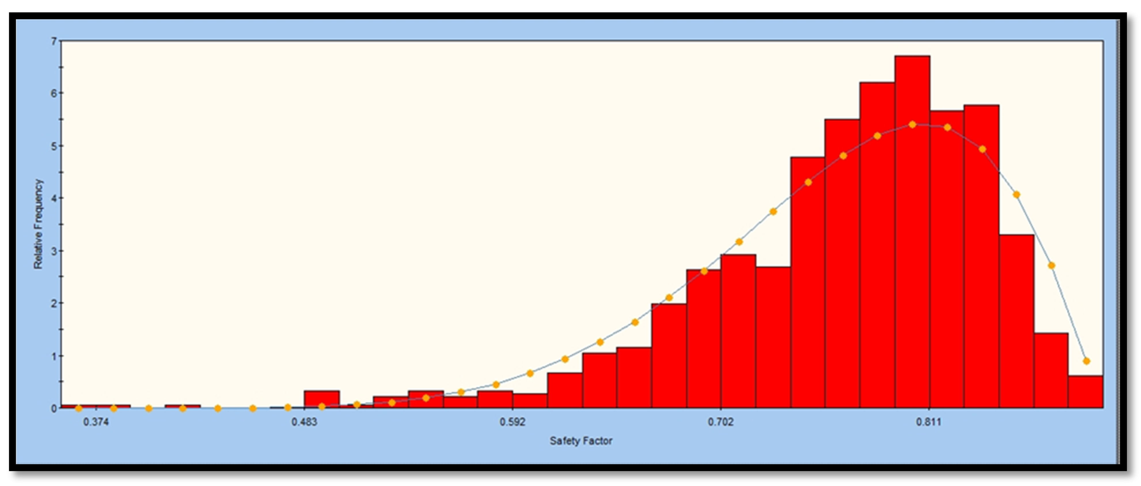
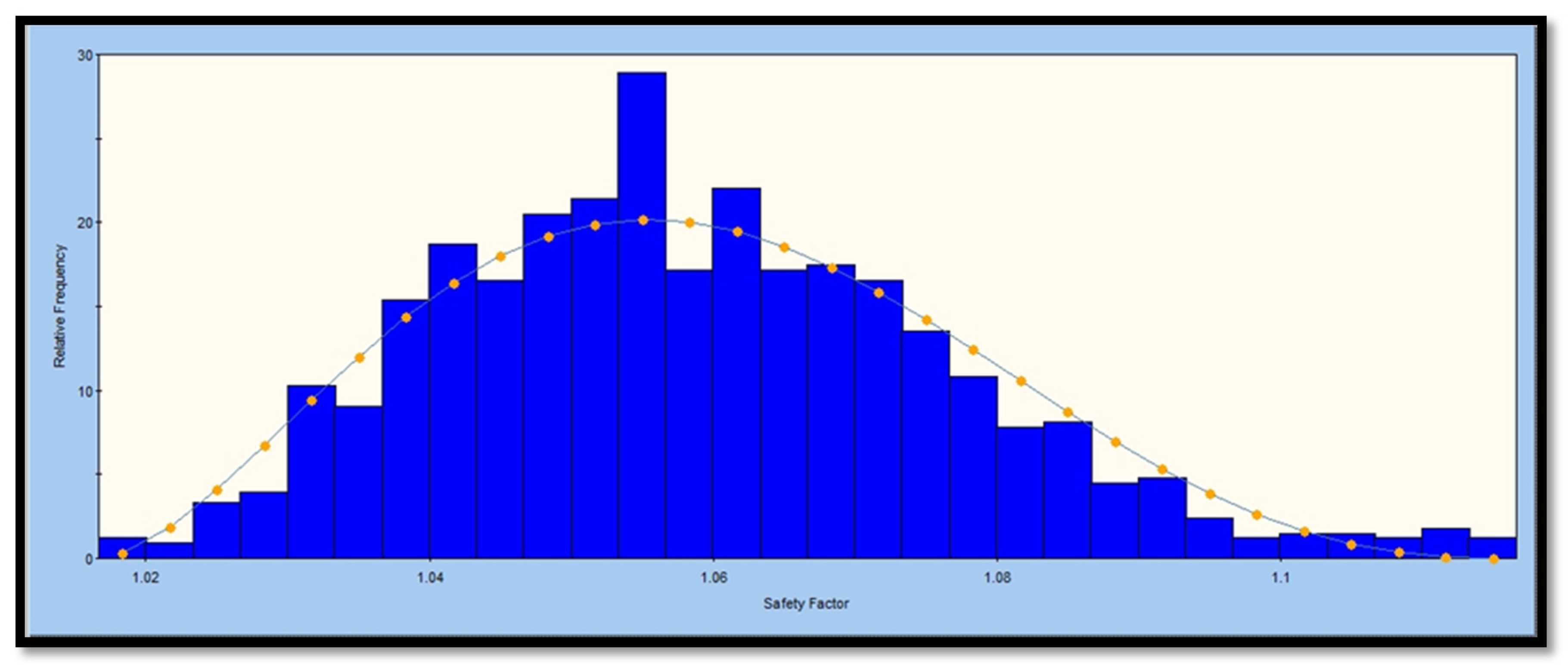
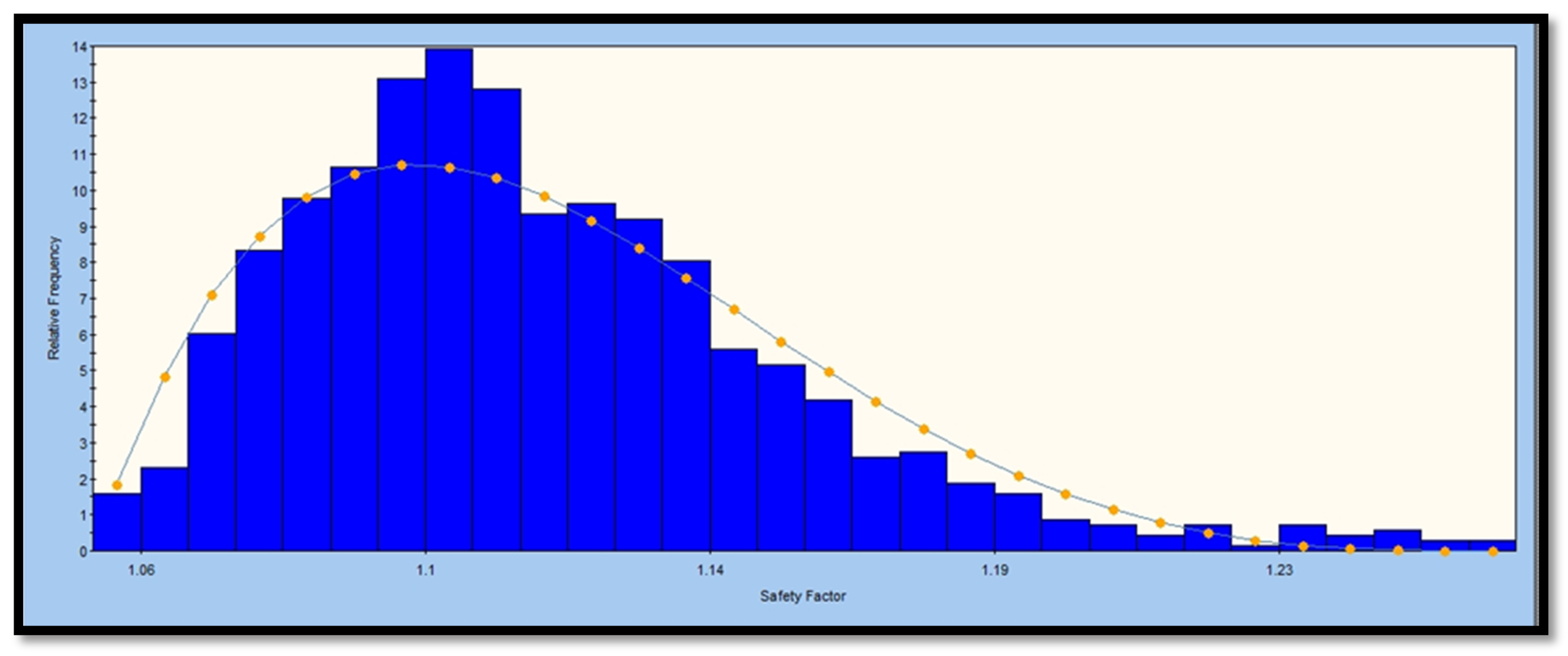
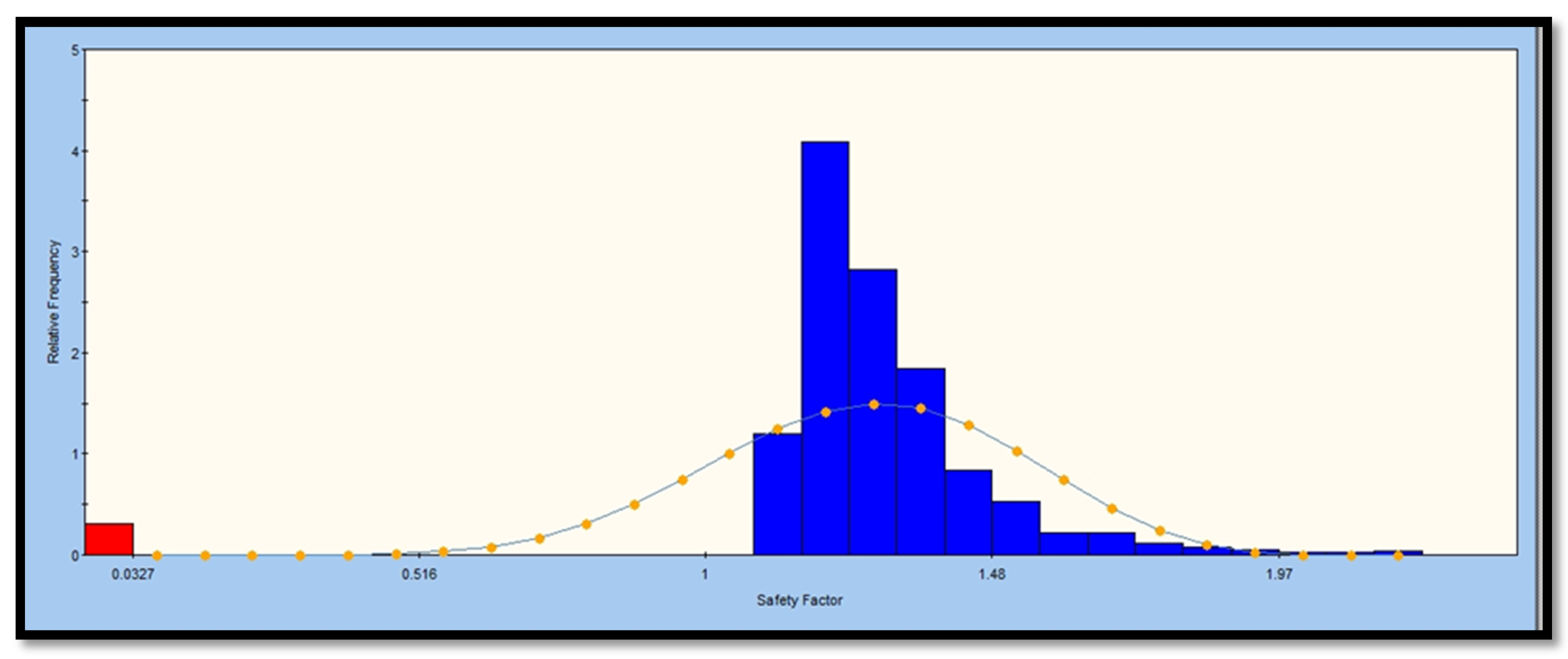
| Parameters | Simulation Per Case | |||||
|---|---|---|---|---|---|---|
| Case A | Case B | Case C | Case D | Case E | Case F | |
| FoS Range | 0.169–0.363 | 0.483–0.811 | 0.725–0.903 | 1.02–1.1 | 1.06–1.23 | 0.0327–1.97 |
| Slope Angle (o) | 90 | 80 | 75 | 50 | 45 | 40 |
Publisher’s Note: MDPI stays neutral with regard to jurisdictional claims in published maps and institutional affiliations. |
© 2020 by the authors. Licensee MDPI, Basel, Switzerland. This article is an open access article distributed under the terms and conditions of the Creative Commons Attribution (CC BY) license (http://creativecommons.org/licenses/by/4.0/).
Share and Cite
Sengani, F.; Mulenga, F. Application of Limit Equilibrium Analysis and Numerical Modeling in a Case of Slope Instability. Sustainability 2020, 12, 8870. https://doi.org/10.3390/su12218870
Sengani F, Mulenga F. Application of Limit Equilibrium Analysis and Numerical Modeling in a Case of Slope Instability. Sustainability. 2020; 12(21):8870. https://doi.org/10.3390/su12218870
Chicago/Turabian StyleSengani, Fhatuwani, and François Mulenga. 2020. "Application of Limit Equilibrium Analysis and Numerical Modeling in a Case of Slope Instability" Sustainability 12, no. 21: 8870. https://doi.org/10.3390/su12218870
APA StyleSengani, F., & Mulenga, F. (2020). Application of Limit Equilibrium Analysis and Numerical Modeling in a Case of Slope Instability. Sustainability, 12(21), 8870. https://doi.org/10.3390/su12218870