A Flexible Tool for Modeling and Optimal Dispatch of Resources in Agri-Energy Hubs

Abstract

The dispatch of energy and resources in agricultural systems often involves the definition and resolution of optimization problems. This paper presents a novel tool composed of a set of MATLAB^® and Simulink^® files that has been developed to ease such tasks. In contrast to other alternatives, it allows the consideration of multiple kinds of resources in the problem and the relationships between the inputs and outputs of the system; its parametrization can be defined graphically in Simulink^® without requiring third party software, and the entire package is freely available on Github. The package can generate the constraints in MATLAB^® code and can get the optimal dispatch schedule for the deterministic mixed-integer linear problem that represents the defined system. Its main functions and blocks as well as a case study based on a traditional Mediterranean greenhouse and a photovoltaic parking lot located in Almeria (Spain) are included to demonstrate its use and clarify how the problem is formulated. The simulation performed validates the tool as being useful for decision-making (schedule irrigation and CO₂ enrichment, as well as managing storage systems) in these and similar environments. Future implementations are intended to incorporate the interconnection of agents with opposed interests and robust optimization strategies for uncertain scenarios.

1. Introduction

Today’s realization that the energy sector must move towards a more efficient, affordable, reliable, safe, and sustainable system is encouraging research on the generation, transport, consumption, and storage processes [1]. Many authors postulate that decentralized and distributed approaches may exploit the local renewable energy sources [2] and combine different energy carriers, which results in a synergy that contributes to the sector’s development [3]. In this regard, the energy hub (EH) concept [4] arose in 2006 for designating production systems with the latter characteristic (although most works include RES as well, but this is not something inherent to the EH’s definition). Geidl and Andersson defined it as “the interface between producers, consumers, and transport infrastructure, which, from the point of view of a system, provides the relationship between the inputs, outputs, conversion, and storage of different energy carriers” [5]. Over the last years, the number of papers related to EHs has been constantly growing, as supported by some of the reviews that give an overview on this topic [6,7], and the term has settled down as well as others, such as microgrid (MG), virtual power plant (VPP), or multi-energy system (MES), which tend to appear in similar energy dispatch problems [8].

A quick look at some of the latest works related to distributed generation shows that most of them rely on solving optimization problems either for design or management purposes. For instance, particle swarm optimization (PSO) was used to obtain the optimal scheduling of a hybrid (thermal and electric) system [9] and to size ten grid-connected hybrid blocks aimed at reducing the supply deficit in Sierra Leone [10]. Model predictive control (MPC) is also associated with control problems in this kind of system: It has been applied to the optimal operation of hybrid power systems in the sugar cane industry [11], and more recently to networked microgrids [12,13] and desalination processes [14].

This is germane to the field of precision agriculture and agro-industrial production districts, where the growing concern about overexploitation of exhaustible resources and the need to maintain the modern economy and quality of life have raised new challenges for scientists. In terms of energy waste, the economic impact of the underlying ground during the production period has been analyzed in facilities such as broiler houses [15]. Another concern, particularly in greenhouses, is that energy consumption seems to have settled down as a significant factor that hinders their development [16], and many proposals have started to tackle dispatch problems from a wider perspective, that is, integrating all the resources required for crop development (water, energy, CO₂, etc.); just to cite a few examples: optimally using combined heating and power facilities [17], determining the operation scheduling of a greenhouse with CO₂ enrichment and artificial lighting [18], or managing water production and its use [19,20].

The ODEHubs (Optimal Dispatch for Energy Hubs) tool developed during the CHROMAE project [21] by the authors of this paper—from the Automatic Control, Robotics, and Mechatronics Research Group (TEP-197) [22]—aims to contribute to the optimal management of these resources in a way that ensures equitable access, efficiency, and sustainability in agro-industrial districts. To put ODEHubs’s features into context, the following paragraphs outline some related software packages as well as their strengths and weaknesses.

At present, many of the multifarious tools of interest that cope with these issues have been encompassed in reviews on district-scale [23] and urban [24] energy systems, where the spotlight is mainly on consolidated and specific engineering software for design and analysis. Other reviews focused on broader contexts [25,26] comprise less mature applications that rely on general-purpose programming environments or languages—such as CPLEX [27], GAMS [28], AMPL [29], AIMMS [30], MATLAB^® [31], R [32], or Python [33]—and even, sometimes, on the self-learning capacity of the users. To the authors’ knowledge, MATLAB^® is extensively employed in this field of research, both as a standalone version and combined with other optimization-assisted modeling tools. It happens to be one the more common programming languages as well, together with Python and GAMS [25], but despite its potential, to date, very few specific tools for dealing with the most common problems in EHs have been developed and made freely available.

• Ehub Modeling Tool [34]. This consists of a set of MATLAB^® scripts for creating input case study data, which are sent and then executed in the optimization package AIMMS. It also incorporates R code for visualizing the results of the simulations. A subsequent version was released in Python, which includes a graph-based modeling tool. Software available at: https://github.com/hues-platform/ehub-modeling-tool.
• EHCM Toolbox [35]. An object-oriented programming tool that was conceived to deal with the control necessities of a building and entirely in MATLAB^®. Consequently, it might lack flexibility in certain aspects, which is counterbalanced by a sophisticated model for batteries and the possibility to integrate detailed building dynamics from another toolbox. Software available at: https://control.ee.ethz.ch/software/BRCM-Toolbox1.html.
• MATPOWER Optimal Scheduling Tool [36] (MOST). This is an extension of the MATPOWER package, a free and open-source set of MATLAB^® files for solving steady-state electric power scheduling problems. MOST can be used to solve from simple deterministic unconstrained problems to stochastic, security-constrained, combined unit-commitment, and multi-period optimal power flow problems. The current implementation is limited to DC power flow modeling of the network, so it is a bit limited when it comes to multi-energy systems (MESs) and EHs. Software available at: https://github.com/MATPOWER/most.
• IMAKUS [37]. This is the name given to a deterministic model of the German power system aimed at making investment decisions on storage and conventional generation assets. Although it was implemented in MATLAB^® code using a generic formulation, its authors do not clarify its possible use on other regions or with other resources than electricity. No support website.
• LUSYM [38]. A tool quite similar to MOST in the sense that it is focused on the electricity sector and allows the introduction of nearly the same constraints in the problem. The main difference resides in the use of GAMS together with MATLAB^®, which are interfaced so that GAMS is used for solving the optimization problem and MATLAB^® for processing the input and output data. No support website.
• EUPowerDispatch [39]. This is another tool for the optimal dispatch of the power system, but particularized at the European level, and it uses GAMS and MATLAB^® in the same way that LUSYM does. More information available at: https://ses.jrc.ec.europa.eu/eupowerdispatch-model.
• Software Library for Multi-Energy Systems (an official name has not been given yet) [40]. This is probably the most flexible and complete of the alternatives, is based on object-oriented programming, and is derived from the generalized modeling framework for MESs proposed by Long. It is intended to be used for MPC applications rather than scheduling problems. The same version was built both in Python and MATLAB^®, although none of them is freely available. No support website.

All of these tools have contributed in one way or another to establishment of the basis from which developers can keep providing new algorithms and procedures to the field of energy and resource management. Nonetheless, there is still room for improvement in certain aspects that the researchers might demand: Less experienced users might struggle with coding, and there exists no graph-based modeling tool for the MATLAB^® environment that allows one to formulate and solve resource dispatch problems; four out of the seven packages are focused on purely electric systems (3,4,5,6), only three are freely available online and properly documented (1,2,3), and some of them require third-party software that is subject to a license (1,5,6).

Thus, given the current alternatives, ODEHubs constitutes a tool with significant improvements. First, multiple carriers can be considered in the dispatch problem thanks to the general model for EHs and MESs [41] that has been incorporated, and, what is more important, the system can be defined via Simulink^® blocks, by analogy with its input–output graph representation, or with MATLAB^® code. Second, it allows the users to choose between two optimization modes and different solvers: on the one hand, MPC-based (receding horizon strategy) or scheduling (fixed horizon); on the other, the internal MATLAB^® function intlinprog, so no third-party software installation is required, or any compatible external solver through YALMIP [42] (for instance, CPLEX [27]). Finally, the set of MATLAB^® and Simulink^® files that compose this tool are freely available on Github (https://github.com/ual-arm/odehubs), together with the ‘ready-to-use’ data-set of the case study presented in Section 4. Other contributions of this work are the extension of the prior general model [41] in order to add device-dependent variable loads and providing an example of the use of the tool in a case study with real-world data of a traditional Mediterranean greenhouse.

The remainder of this paper is organized as follows: Section 2 presents the model coded to solve the optimization problem; Section 3 contains a description of the main modules and their configuration parameters; Section 4 shows an example case where the ODEHubs toolbox is employed to obtain the operation schedule for the greenhouse and its facilities; Section 5 analyzes the current drawbacks of ODEHubs and future enhancements.

2. Conversion and Storage Model

The preliminary version of the ODEHubs model was formulated and published in a previous study [41], to which readers are referred for clarification, and has been kept without meaningful changes. In broad terms, the models of most energy hubs represent energy and mass balances between a set of input resources that can be transformed into another set of output resources. The basic relationship proposed by [5] is based on a coupling matrix C that represents the conversion process between multiple energy carriers in steady state ($\mathit{L}-\mathit{CP}=0$), where $\mathit{P}$ are the input powers or sources and $\mathit{L}$ the output powers or loads. The coefficients of this matrix are given by the product of the efficiencies of all the conversion units or devices that intervene in the conversion and the so-called dispatch factors that need to be introduced whenever one energy carrier splits up to several flows inside the EH. Additional constraints may consider power limits, the presence of storage systems, and necessary energy balances among these dispatch factors. This has led to formulations that have progressively introduced elements to represent conversion and storage processes more accurately, but share a similar basis, as [41] discussed in the reference study [41]. In contrast to other proposals in the literature, the so-called “path vector” was defined to consider a decision variable for each possible path between inputs and outputs and to avoid the non-linear relationships of [5]’s model when two dispatch factors are multiplied in the coupling matrix [5]. The input and internal flows are obtained from the elements of the path vector and suitably defined coupling matrices. Some outputs or loads can be considered dependent on the fact that a certain device is turned on or off, which was taken into account by arranging [5]’s equation $\mathit{L}-\mathit{CP}=0$. All the equations from [41] that encompass these and other circumstances are presented below, although, for the sake of simplicity, some of them will appear here in matrix notation. In addition, the term “power” will be superseded by “flow” or just omitted, since not only energy carriers are considered, but also material resources.

2.1. Prior Formulation

Consider a general energy hub with $N_i$ input flows, $N_o$ output flows, $N_p$ paths between these inputs and outputs, $N_d$ conversion devices with a total amount of $N_{di}$ input flows and $N_{do}$ output flows, and discrete time models using a uniform sample time $T=t(k+1)-t\left(k\right)$, where k constitutes any discrete time instant.

The conversion and storage processes need to satisfy balance conditions at each time step and between consecutive time steps, respectively, as stated in Equations (1) and (2):

$${\mathit{\delta }}_{\mathit{O}}\left(k\right)\mathit{O}\left(k\right)+\mathit{M}\left(k\right)=\mathit{C}\left(k\right)\mathit{P}\left(k\right)-{\mathit{Q}}_{\mathit{ch}}\left(k\right)+{\mathit{Q}}_{\mathit{dis}}\left(k\right),$$

(1)

$$\mathit{S}(k+1)={\mathit{C}}_{\mathit{S}}\left(k\right)\mathit{S}\left(k\right)+{\mathit{C}}_{\mathit{ch}}\left(k\right){\mathit{Q}}_{\mathit{ch}}\left(k\right)-{\mathit{C}}_{\mathit{dis}}\left(k\right){\mathit{Q}}_{\mathit{dis}}\left(k\right),$$

(2)

where $\mathit{P}$ is the $N_p\times 1$ vector of flows between inputs and outputs, $\mathit{M}$ is the $N_o\times 1$ vector of market sales flows, $\mathit{O}$ is the $N_o\times 1$ vector of output flows, ${\mathit{Q}}_{\mathit{ch}}$ is the $N_o\times 1$ vector of charge flows, ${\mathit{Q}}_{\mathit{dis}}$ is the $N_o\times 1$ vector of discharge flows, $\mathit{S}$ is the $N_o\times 1$ vector of stored resources, $\mathit{C}$ is the $N_o\times N_p$ coupling matrix, ${\mathit{C}}_{\mathit{ch}}$ is the $N_o\times N_o$ diagonal matrix of charge efficiencies, ${\mathit{C}}_{\mathit{dis}}$ is the $N_o\times N_o$ diagonal matrix of discharge efficiencies, ${\mathit{C}}_{\mathit{S}}$ is the $N_o\times N_o$ diagonal matrix of resource degradation, and ${\mathit{\delta }}_{\mathit{O}}$ is the $N_o\times N_o$ binary diagonal matrix of output activation.

Additionally, the relationship between the internal $\mathit{P}$ vector flows and both the input flows to the EH itself must be established, as defined in Equation (3), as well as the input–output flows in each device, as given in Equations (4) and (5):

$$\mathit{I}\left(k\right)={\mathit{C}}_{\mathit{i}}\mathit{P}\left(k\right),$$

(3)

$${\mathit{D}}_{\mathit{i}}\left(k\right)={\mathit{C}}_{\mathit{di}}\left(k\right)\mathit{P}\left(k\right),$$

(4)

$${\mathit{D}}_{\mathit{o}}\left(k\right)={\mathit{C}}_{\mathit{do}}\left(k\right)\mathit{P}\left(k\right),$$

(5)

where $\mathit{I}$ is the $N_i\times 1$ vector of input flows, ${\mathit{D}}_{\mathit{i}}$ is the $N_{di}\times 1$ vector of devices’ flows (referred to their inputs), ${\mathit{D}}_{\mathit{o}}$ is the $N_{do}\times 1$ vector of devices’ flows (referred to their outputs), ${\mathit{C}}_{\mathit{i}}$ is the $N_i\times N_p$ input coupling matrix, ${\mathit{C}}_{\mathit{di}}$ is the $N_{di}\times N_p$ device coupling matrix (referred to their inputs), and ${\mathit{C}}_{\mathit{do}}$ is the $N_{do}\times N_p$ device coupling matrix (referred to their outputs). Note that in Ref. [41], only one equation was defined, instead of two, to limit the flows through the devices of the EH.

Except vector $\mathit{O}$, which a priori does not contain decision variables (see next subsection for the opposite case), and vector $\mathit{P}$, which is indirectly limited by the production capacity of the conversion devices from the following equations, the remaining vectors need to be constrained in order to ensure that the resource conversion and storage devices do not exceed their defined capacities. That is the raison d’être of Equations (6)–(12):

$${\mathit{M}}^{\mathit{min}}\left(k\right){\mathit{\delta }}_{\mathit{M}}\left(k\right)\le \mathit{M}\left(k\right)\le {\mathit{M}}^{\mathit{max}}\left(k\right){\mathit{\delta }}_{\mathit{M}}\left(k\right),$$

(6)

$${\mathit{I}}^{\mathit{min}}\left(k\right){\mathit{\delta }}_{\mathit{I}}\left(k\right)\le \mathit{I}\left(k\right)\le {\mathit{I}}^{\mathit{max}}\left(k\right){\mathit{\delta }}_{\mathit{I}}\left(k\right),$$

(7)

$${\mathit{D}}_{\mathit{i}}^{\mathit{min}}\left(k\right){\mathit{\delta }}_{{\mathit{D}}_{\mathit{i}}}\left(k\right)\le {\mathit{D}}_{\mathit{i}}\left(k\right)\le {\mathit{D}}_{\mathit{i}}^{\mathit{max}}\left(k\right){\mathit{\delta }}_{{\mathit{D}}_{\mathit{i}}}\left(k\right),$$

(8)

$${\mathit{D}}_{\mathit{o}}^{\mathit{min}}\left(k\right){\mathit{\delta }}_{{\mathit{D}}_{\mathit{o}}}\left(k\right)\le {\mathit{D}}_{\mathit{o}}\left(k\right)\le {\mathit{D}}_{\mathit{o}}^{\mathit{max}}\left(k\right){\mathit{\delta }}_{{\mathit{D}}_{\mathit{o}}}\left(k\right),$$

(9)

$${\mathit{Q}}_{\mathit{ch}}^{\mathit{min}}\left(k\right){\mathit{\delta }}_{\mathit{ch}}\left(k\right)\le {\mathit{Q}}_{\mathit{ch}}\left(k\right)\le {\mathit{Q}}_{\mathit{ch}}^{\mathit{max}}\left(k\right){\mathit{\delta }}_{\mathit{ch}}\left(k\right),$$

(10)

$${\mathit{Q}}_{\mathit{dis}}^{\mathit{min}}\left(k\right){\mathit{\delta }}_{\mathit{dis}}\left(k\right)\le {\mathit{Q}}_{\mathit{dis}}\left(k\right)\le {\mathit{Q}}_{\mathit{dis}}^{\mathit{max}}\left(k\right){\mathit{\delta }}_{\mathit{dis}}\left(k\right),$$

(11)

$${\mathit{S}}^{\mathit{min}}\left(k\right)\le \mathit{S}\left(k\right)\le {\mathit{S}}^{\mathit{max}}\left(k\right),$$

(12)

where the superscripts max and min refer to the lower or upper limit of each vector (for instance, ${\mathit{S}}^{\mathit{max}}$ determines the maximum amount that each storage system may store), and the rest of the $\delta$ symbols define diagonal binary variables that indicate if the flow is allowed or not. In particular, ${\mathit{\delta }}_{\mathit{M}}$ is the $N_o\times N_o$ binary diagonal matrix of market sales flow activation, ${\mathit{\delta }}_{\mathit{I}}$ is the $N_i\times N_i$ binary diagonal matrix of input flow activation, ${\mathit{\delta }}_{{\mathit{D}}_{\mathit{i}}}$ is the $N_{di}\times N_{di}$ binary diagonal matrix of devices’ flow activation (referred to their inputs), ${\mathit{\delta }}_{{\mathit{D}}_{\mathit{o}}}$ is the $N_{do}\times N_{do}$ binary diagonal matrix of devices’ flow activation (referred to their outputs), ${\mathit{\delta }}_{\mathit{ch}}$ is the $N_o\times N_o$ binary diagonal matrix of charge flow activation, and ${\mathit{\delta }}_{\mathit{dis}}$ is the $N_o\times N_o$ binary diagonal matrix of discharge flow activation.

Additional constraints are required in order to take into account certain processes that cannot occur simultaneously. Three situations can be distinguished: preventing the charge and discharge of the same storage systems, by means of Equation (13):

$${\mathit{\delta }}_{\mathit{ch}}\left(k\right)+{\mathit{\delta }}_{\mathit{dis}}\left(k\right)\le \mathbf{1},$$

(13)

where $\mathbf{1}$ is the identity matrix (note that $\mathit{I}$ already denotes a variable of the model); avoiding the use of the same infrastructure for acquiring and selling resources, as expressed in Equation (14):

$${\delta }_{I,i}\left(k\right)+{\delta }_{M,o}\left(k\right)\le 1,$$

(14)

where i and o respectively denote the elements of ${\mathit{\delta }}_{\mathit{M}}$ and ${\mathit{\delta }}_{\mathit{I}}$ with common infrastructure; and impeding that some devices operate simultaneously, as stated in Equation (15):

$${\delta }_{D,d^{\left(1\right)}}\left(k\right)+\cdots +{\delta }_{D,d^{\left(n\right)}}\left(k\right)\le 1,$$

(15)

where $d^{\left(1\right)}...d^{\left(n\right)}$ refer to the elements of ${\mathit{\delta }}_{{\mathit{D}}_{\mathit{i}}}$ or ${\mathit{\delta }}_{{\mathit{D}}_{\mathit{o}}}$ corresponding to non-simultaneous converters.

Owing to the definition of the path vector, the variables corresponding to the outputs of a device that produces different resources at the same time (e.g., a combined heat and power system or a boiler with carbon capture) must equal the input amount of that device. Equation (16) satisfies that balance:

$$P_{p^{\left(1\right)}}\left(k\right)+...+P_{p^{\left(n\right)}}\left(k\right)=P_{p^{(n+1)}}\left(k\right)+...+P_{p^{\left(m\right)}}\left(k\right),$$

(16)

where $p^{\left(1\right)}...p^{\left(n\right)}...p^{\left(m\right)}$ correspond to simultaneous converter outputs. These situations will be exemplified in Section 4, although readers are encouraged to consult Ref. [41] for a better understanding.

Finally, the cost function of the optimization problem can be written as in Equation (17):

$$\begin{array}{ccc}\hfill & \min \hfill & \hfill {\displaystyle \sum _{k=1}^H(\mathit{C}\left(k\right)\mathit{I}\left(k\right)-\mathit{s}\left(k\right)\mathit{M}\left(k\right))}\\ \hfill & \mathrm{s}.\mathrm{t}.\hfill & \hfill \mathrm{the}\mathrm{aforementioned}\mathrm{constraints},\end{array}$$

(17)

where $\mathit{C}\left(k\right)$ is the $1\times N_i$ vector containing the price of each input, $\mathit{S}\left(k\right)$ is the $1\times N_o$ vector containing the price of sold resources (in terms of energy, mass, or volume), and H is the length (in samples) of the control horizon. Note that, depending on the units of the sample time T and the vectors, additional terms might need to be introduced in Equations (2) and (17) to convert between time units.

2.2. Device-Dependent Fixed and Variable Loads

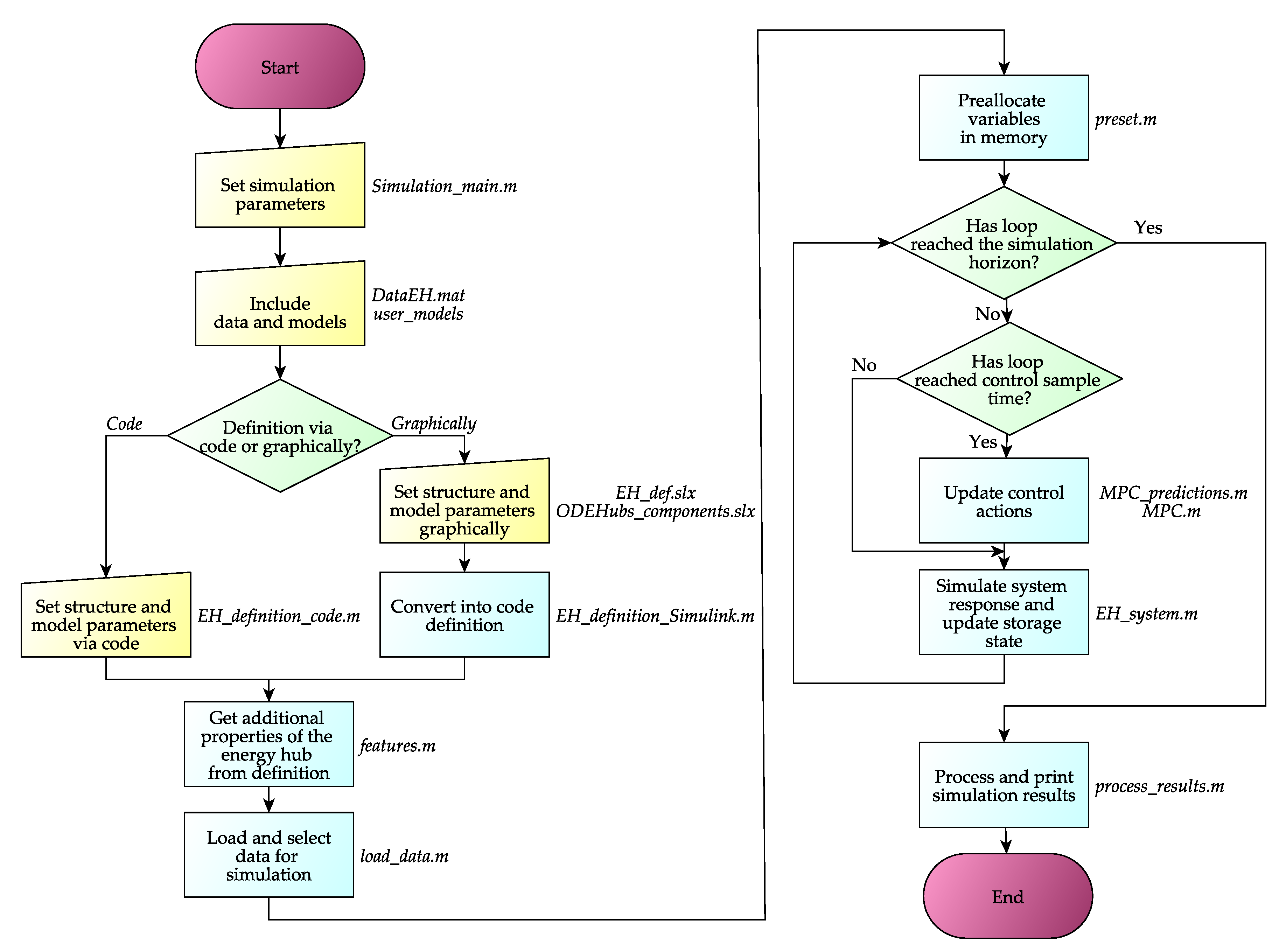
Note that, in the arrangement proposed in Ref. [41], to consider loads coming from the use of a particular device consisted in adding any necessary element to vector $\mathit{O}$ and using ${\mathit{\delta }}_{\mathit{O}}$ in Equation (1). However, this solution is only suitable in the case of fixed demands, since the model does not contemplate the possibility of adding variable demands proportionally to the flow of the device. One straightforward way to iron out this situation consists in redefining the elements of $\mathit{O}$ so that the demand equals the proportional flow of the device or, in what turns out to be equivalent, redefining matrices $\mathit{C}$ and ${\mathit{\delta }}_{\mathit{O}}$. In the following paragraphs, both situations are exemplified by using a hypothetical EH in order to elucidate how the previous formulation needs to be adapted, which is relevant for programming.

Let Figure 1 represent a simplified example of an EH where an electric pump is in charge of keeping the water pressure of an irrigation facility. In order to ease the understanding of this example, free water discharge and no electricity storage or market sales flows are considered. The path vector only has two elements, that is, the number of possible paths in the EH: $I_1\to D_1\to O_1$ ($P_1$) and $I_2\to O_2$ ($P_2$), so, in this concrete case, ${\mathit{C}}_{\mathit{i}}$ becomes the identity matrix and $\mathit{P}=\mathit{I}$. Thus, the balance equations of the conversion processes and their limits, i.e., Equations (1), (3)–(5), (8) and (9), adopt the form of Equations (18)–(23):

$$\left[\begin{array}{cc}1& 0\\ 0& {\delta }_{D,1}\left(k\right)\end{array}\right]\left[\begin{array}{c}{O}_1\left(k\right)\\ O_2\left(k\right)\end{array}\right]=\left[\begin{array}{cc}{C}_{1,1}\left(k\right)& 0\\ 0& C_{2,2}\left(k\right)\end{array}\right]\left[\begin{array}{c}{P}_1\left(k\right)\\ P_2\left(k\right)\end{array}\right]-\left[\begin{array}{c}{Q}_{ch,1}\left(k\right)\\ 0\end{array}\right]+\left[\begin{array}{c}{Q}_{dis,1}\left(k\right)\\ 0\end{array}\right],$$

(18)

$$\left[\begin{array}{c}{I}_1\left(k\right)\\ I_2\left(k\right)\end{array}\right]=\left[\begin{array}{cc}1& 0\\ 0& 1\end{array}\right]\left[\begin{array}{c}{P}_1\left(k\right)\\ P_2\left(k\right)\end{array}\right],$$

(19)

$$D_{i,1}\left(k\right)=\left[\begin{array}{cc}1& 0\end{array}\right]\left[\begin{array}{c}{P}_1\left(k\right)\\ P_2\left(k\right)\end{array}\right],$$

(20)

$$D_{o,1}\left(k\right)=\left[\begin{array}{cc}{C}_{1,1}\left(k\right)& 0\end{array}\right]\left[\begin{array}{c}{P}_1\left(k\right)\\ P_2\left(k\right)\end{array}\right],$$

(21)

$$D_{i,1}^{min}\left(k\right){\delta }_{D,1}\left(k\right)\le D_{i,1}\left(k\right)\le D_{i,1}^{max}\left(k\right){\delta }_{D,1}\left(k\right),$$

(22)

$$D_{o,1}^{min}\left(k\right){\delta }_{D,1}\left(k\right)\le D_{o,1}\left(k\right)\le D_{o,1}^{max}\left(k\right){\delta }_{D,1}\left(k\right),$$

(23)

where the non-zero elements of the coupling matrix $\mathit{C}$ and ${\mathit{C}}_{\mathit{do}}$ would be equal to one because no transformation of resources exits in the EH, and ${\mathit{\delta }}_{\mathit{O}}$ contains the binary variable related to the activation of the pump (${\delta }_{D,1}$).

Now, if the electric pump is assumed to have a constant consumption, $O_2$ would be equal to that value instead of constituting a decision variable in the optimization problem, which is the case explained in Ref. [41]. However, if a consumption proportional to the pumped water flow is considered instead, with a constant of proportionality $\kappa$, Equation (18) needs to be reformulated as follows. First, it must be defined whether the consumption is proportional to the inlet or the outlet flow, which would lead to two different expressions: $O_2=\kappa D_{i,1}=\kappa P_1$ or $O_2=\kappa D_{o,1}=\kappa C_{1,1}{D}_{i,1}=\kappa C_{1,1}{P}_1$, respectively. Only the second expression will be used from now on, as it will allow generalizations to the first one. In any case, as both $P_1$ and ${\delta }_{D,1}$ are decision variables, their product would turn the optimization problem into a non-linear one when substituting $O_2$ into Equation (18). To avoid this, ${\delta }_{D,1}$ can be removed from ${\mathit{\delta }}_{\mathit{O}}$ (making that element equal to one), since $P_1$ is already constrained by the on/off state of the pump through Equations (22) and (23), which leads to transformation of Equation (18) into Equation (24):

$$\left[\begin{array}{cc}1& 0\\ 0& 1\end{array}\right]\left[\begin{array}{c}{O}_1\left(k\right)\\ \kappa C_{1,1}\left(k\right)P_1\left(k\right)\end{array}\right]=\left[\begin{array}{cc}{C}_{1,1}\left(k\right)& 0\\ 0& C_{2,2}\left(k\right)\end{array}\right]\left[\begin{array}{c}{P}_1\left(k\right)\\ P_2\left(k\right)\end{array}\right]-\left[\begin{array}{c}{Q}_{ch,1}\left(k\right)\\ 0\end{array}\right]+\left[\begin{array}{c}{Q}_{dis,1}\left(k\right)\\ 0\end{array}\right],$$

(24)

or, equivalently, arranging matrix $\mathit{C}$ into Equation (25):

$$\left[\begin{array}{cc}1& 0\\ 0& 1\end{array}\right]\left[\begin{array}{c}{O}_1\left(k\right)\\ 0\end{array}\right]=\left[\begin{array}{cc}{C}_{1,1}\left(k\right)& 0\\ -\kappa C_{1,1}\left(k\right)& C_{2,2}\left(k\right)\end{array}\right]\left[\begin{array}{c}{P}_1\left(k\right)\\ P_2\left(k\right)\end{array}\right]-\left[\begin{array}{c}{Q}_{ch,1}\left(k\right)\\ 0\end{array}\right]+\left[\begin{array}{c}{Q}_{dis,1}\left(k\right)\\ 0\end{array}\right].$$

(25)

Just to recap all of the above and as a rule of thumb, in case of device-dependent variable demands, the following modifications must be performed in the model presented previously [41]—removing from ${\mathit{\delta }}_{\mathit{O}}$, by making equal to one, all the elements of its diagonal related to those demands; setting to zero the analogous rows in $\mathit{O}$; and including in the columns of $\mathit{C}$ related to that device the suitable conversion/transformation coefficients multiplied by the negative constant of proportionality between the demand and the flow through the device. Part of the ODEHubs code was generated to perform these modifications in the model.

3. ODEHubs Toolbox

ODEHubs consists of a set of functions and files that allow one to obtain the optimal dispatch or scheduling of any system that can be modeled according to the above-presented equations. Users can manually define the characteristics of this one (number of elements, flow relationship, etc.) and configure certain parameters depending on their needs. In order to serve as a short guide for anyone interested in the tool, the main functions and settings are described in the following lines, considering the general flowchart of the software presented in Figure 2), although specific documentation will be made available on the website of the tool (https://github.com/ual-arm/odehubs).

The first step required to use ODEHubs, and from which the model is generated and adapted to be introduced in the optimization solver, consists in defining the problem, which involves manipulating three or four files, depending on whether the problem is defined graphically or by programming (see their names next to yellow trapezia in Figure 2). Except for Simulation_main.m, which is placed in the root directory, the rest of them can be found in the definition folder. Note also that although the manual procedures, which are described below, have been included sequentially in Figure 2, they are actually interchangeable.

• Simulation_main.m is the base of the flowchart and is where most functions are called. At the beginning of the file, a set of parameters, whose use is clarified below, are declared, and users might need to modify these lines prior to simulation. A struct variable called EH is created during its execution and used to store variables and communicate them to other functions.
• DataEH.mat is a file in the binary data container format that the MATLAB^® program uses, with a single timetable variable called dataEH stored in it. This type of variable allows the grouping of column-oriented data in a table where each row represents a date and time. Thus, the columns consist of all the time-dependent variables required to simulate the system, such as the demanded outputs or weather conditions. Users are responsible for including the data that they need in this format, with the freedom to choose the name of each column/variable. Columns may be empty if no data are required to be loaded, but the timetable needs to be generated according to the simulation start time and horizon (see these parameters’ definition below).
• The folder user_models contains any function that users might need to define time-variable parameters in Equations (1)–(17). They need to be arranged following the syntax parameter = function (data, date, samples, tm), so that parameter is a vector of values obtained from data (which is an automatically filtered version of dataEH) starting at the time declared in date in each tm period of time during the horizon samples.
• EH_definition_code.m is the function employed to set the properties of the energy hubs, and it includes the parameters related to Equations (1)–(17) via MATLAB^® code. The file provided by the authors of this work for the case study presented in Section 4 can be used as a template for other systems just by adapting its content.
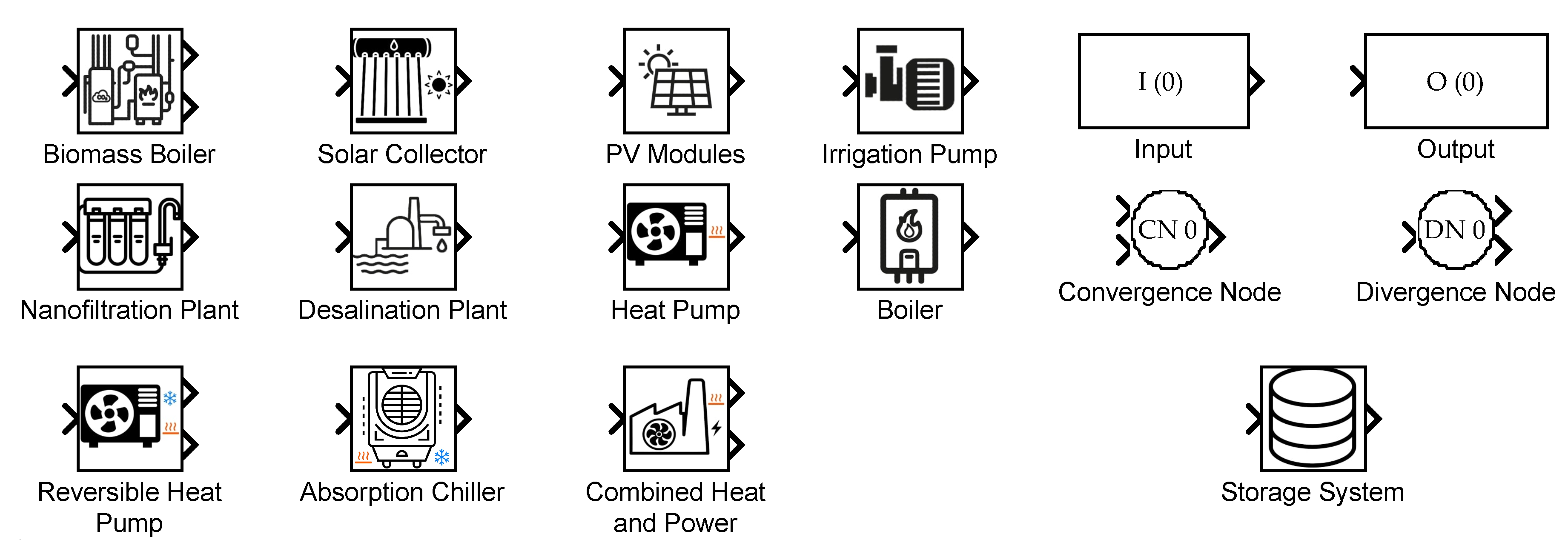
• ODEHubs_components.slx is the Simulink^® library, which, with the support of the user_models folder, incorporates the predefined models of several storage and conversion devices developed during the CHROMAE project [21] (Figure 3). Its blocks, which are described in the next subsection, are employed to build Simulink^® models that represent any EH either by copying and pasting from the library or by dragging from the library browser if ODEHubs_components.slx is added. As in any other library, the file is locked when first opened, but users, and even the developers in future releases of ODEHubs, might add new blocks if necessary.
• EH_def.slx is the default name given to the Simulink^® model employed to define the EH graphically, although any other syntactically valid name can be used if specified in Simulation_main.m, which easily allows one to change between different EHs in each simulation. The case study presented in Section 4 constitutes an example of how to build and configure this file.

The remainder functions are not intended to interact with the users directly, but they are part of the automatic process of calculating the dynamic of the EH and storing and displaying the final results. They are distributed in different folders according to their purpose, but all of them appear in Simulation_main.m and are responsible for calling other specific functions. EH_definition_Simulink.m, features.m, and preset.m arrange the input data from the users to be processed by other functions; load_data.m loads the content of DataEH.mat and filters it by time according to values specified by the users; MPC_predictions.m and MPC.m provide an updated dispatch of the EH’s resources at each sample time specified for the control actions; EH_system.m simulates the response of the EH at each sample time specified for the system’s dynamic; and process_results.m aggregates the flows during the simulation horizon and displays the scheduled dispatch. At this point, note that including MPC_predictions.m and EH_system.m is a mere formal aspect because they currently make use of the same models and variables; thus, the control layer’s dynamic will always match the one of the systems (except if different sample times are chosen for them). However, they will be useful in future releases of ODEHubs, which are expected to incorporate capabilities to simulate non-deterministic scenarios as well as different control strategies that deal with uncertainty.

3.1. ODEHubs’s Block Library

The model presented in Section 2 can be configured both graphically and via code, and, in either case, the parameters that need to be introduced in ODEHubs are related to the elements of the above matrices, that is, the technical features of the devices that compose the EH. ODEHubs’s block library will be used in this section to elaborate on that, since it might be more intuitive than programming code. Figure 3 shows the types of blocks that need to be used in the definition diagram, which were designed based on the elements found in the model presented in Section 2.2 and the appearance of the descriptive diagrams in many works related to EHss (see Figure 1, for example). They can be classified as follows.

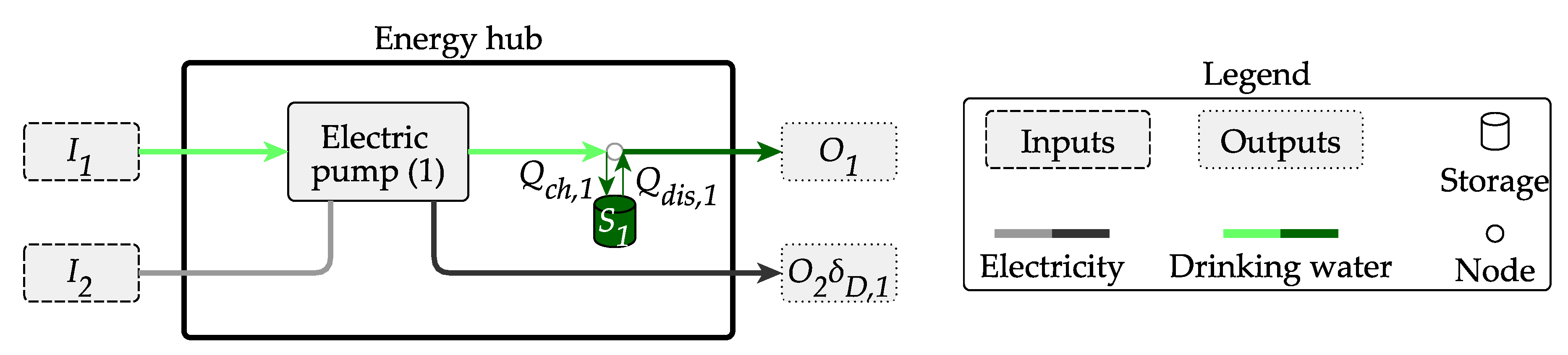
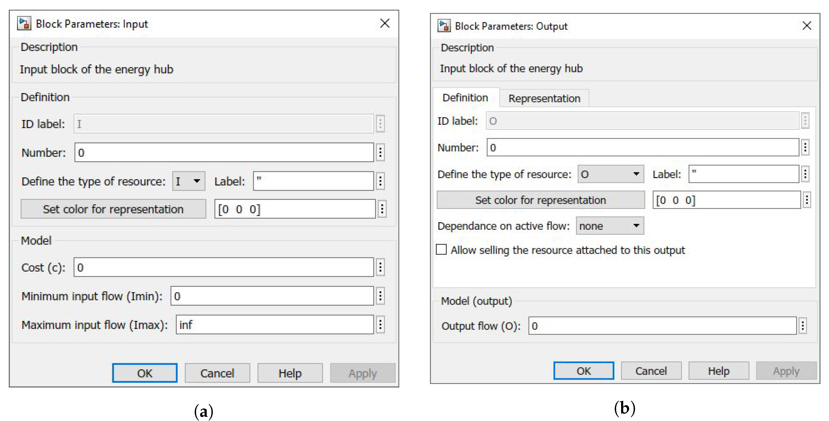
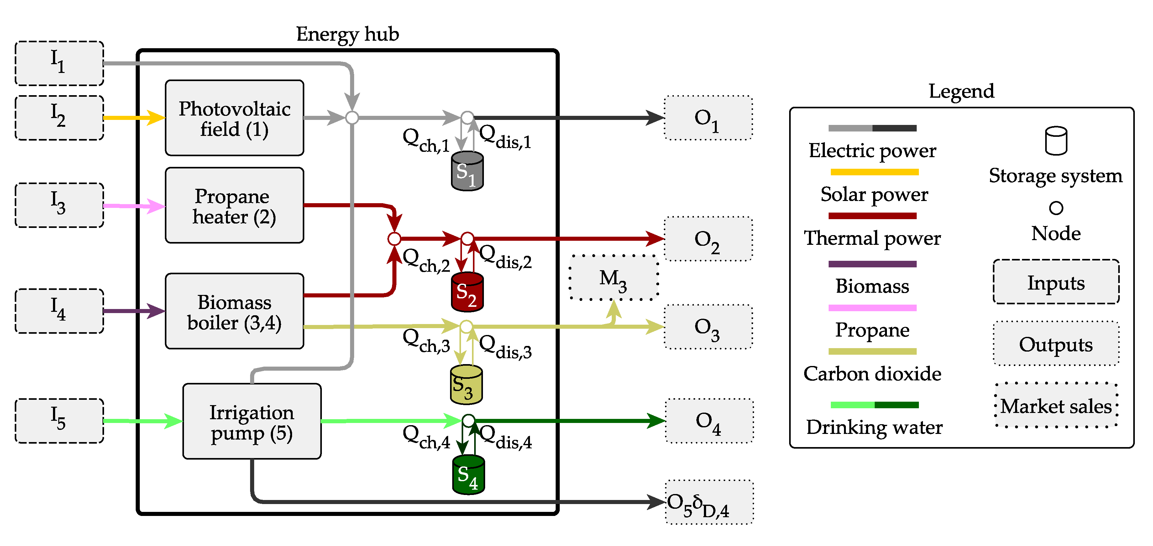
• $N_i$Input blocks (Figure 4a) characterize the available resources of the EH. Their main parameters are the cost of acquiring the resource, part of vector $\mathit{C}$, and the maximum and minimum values of the input flow, which compose vectors ${\mathit{I}}^{\mathit{max}}$ and ${\mathit{I}}^{\mathit{min}}$.
• $N_o$Output blocks (Figure 4b) characterize the loads or demands of the EH. Their main parameter is the value of this flow, part of vector O, or, alternatively, the constant of proportionality mentioned in Section 2.2, if it is a variable device-dependent load. The mask of these blocks allows the definition of this dependence as well as the sale of resources through that output, in which case additional parameters are made visible and editable: the price of selling the resource, part of vector $\mathit{S}$, and the maximum and minimum values of the market flow, which compose vectors ${\mathit{M}}^{\mathit{max}}$ and ${\mathit{M}}^{\mathit{min}}$.
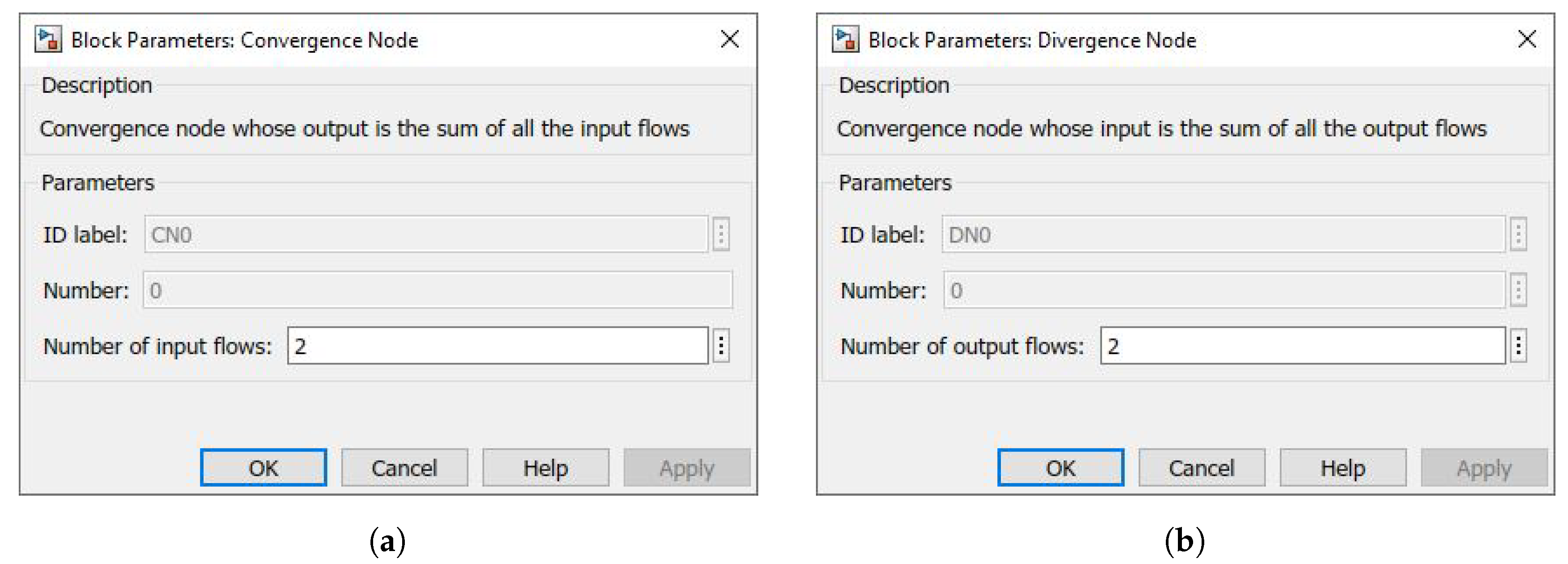
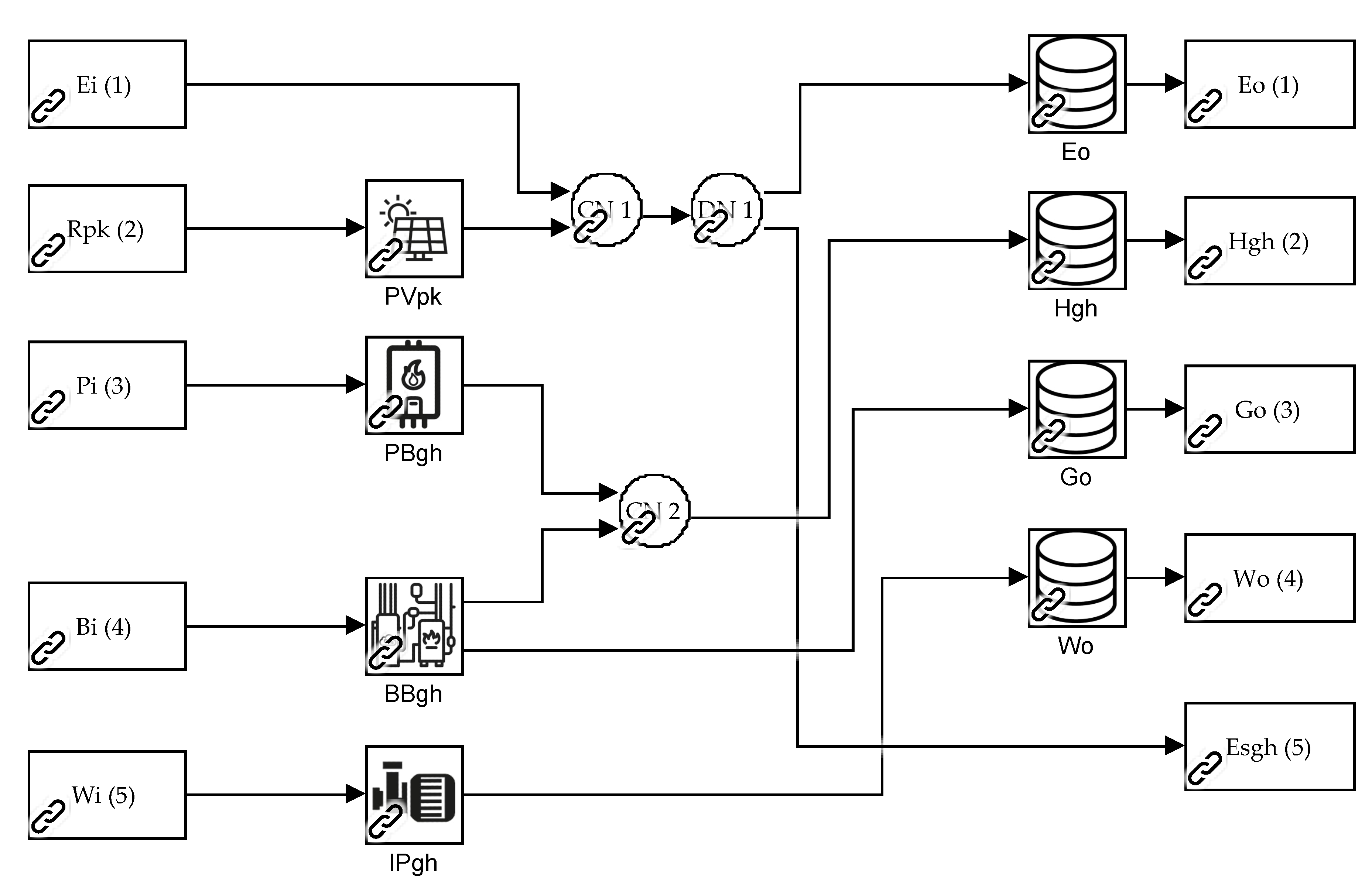
• convergence Node and Divergence Node blocks (Figure 5) do not currently have any utility and, in practice, could be omitted, but, because of the way Simulink^® treats the signals between blocks, they will be needed in future releases of ODEHubs to allow users to merge and split flows numerically in simulations via Simulink^®. For this reason, the diagrams must incorporate these blocks at any time that several flows converge into a single flow (so the sum of the original flows equals the resulting flow) or whenever a flow diverges into different sub-flows (so the sum of the sub-flows equals the original flow). Their only configurable parameter is the number of converging or diverging flows, respectively.
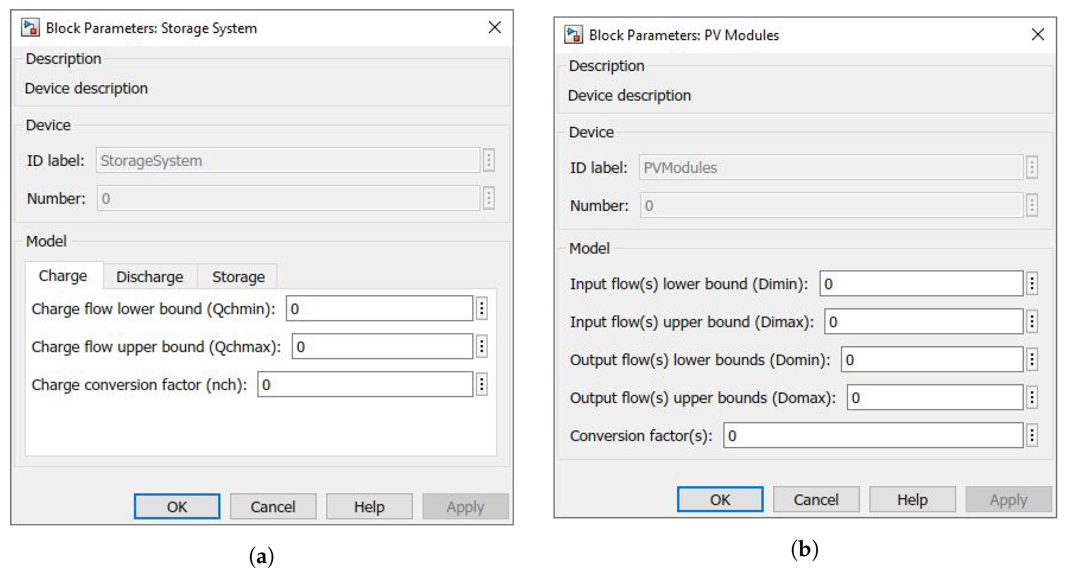
• $N_o$ or less Storage System blocks (Figure 6a) need to be used to characterize the storage devices of the EH. The output of each of these blocks must be connected any Output block where energy, mass, or volume is stored. Their parameters, which are arranged in tabs, allow the definition of the charge and discharge flows and the capacity of each storage system, so they are elements of the vectors ${\mathit{Q}}_{\mathit{ch}}^{\mathit{min}}$, ${\mathit{Q}}_{\mathit{ch}}^{\mathit{max}}$, ${\mathit{Q}}_{\mathit{dis}}^{\mathit{min}}$, ${\mathit{Q}}_{\mathit{dis}}^{\mathit{max}}$, ${\mathit{S}}^{\mathit{min}}$, and ${\mathit{S}}^{\mathit{max}}$; they also allow the definition of the efficiency of each storage process, taking part of the matrices ${\mathit{C}}_{\mathit{ch}}$, ${\mathit{C}}_{\mathit{dis}}$, and ${\mathit{C}}_{\mathit{S}}$. Additionally, the initial state of the storage system must be defined $\mathit{S}\left(0\right)$ in the Storage tab.
• $N_d$ blocks (Figure 6b) corresponding to devices need to be included in the Simulink^® model employed to define the EH graphically. As depicted in Figure 3, ODEHubs’s library consists of some predefined blocks with the same parameters: limits for the input(s) and output(s) of each device related to vectors ${\mathit{D}}_{\mathit{di}}^{\mathit{min}}$, ${\mathit{D}}_{\mathit{di}}^{\mathit{max}}$, ${\mathit{D}}_{\mathit{do}}^{\mathit{min}}$, and ${\mathit{D}}_{\mathit{do}}^{\mathit{max}}$, and the conversion factor(s) between them, which are required to build matrices $\mathit{C}$, ${\mathit{C}}_{\mathit{di}}$, and ${\mathit{C}}_{\mathit{do}}$.

From the above parameters, the ones related to the model can be defined in one of the following ways: as a numeric data type in the case of static coefficients, as a string containing the name of a variable of the dataEH timetable corresponding to the value of such parameter at each sample time, as a string containing the name of a function in the folder user_models, which provides the value of this parameter at each sample time, or as a cell array composed of one or several of the latter ones, which is mandatory for those devices with more than one output, such as the Reversible Heat Pump, the Biomass Boiler, and the Combined Heat and Power blocks.

3.2. Main Configuration Parameters

Apart from setting the model’s parameters, ODEHubs’s users might want to customize the output of the program in order to suit their needs. Among the configuration parameters, one can select if third-party solvers are invoked, define the solver’s options, select the start date for simulation (dataEH needs to be accordingly defined) and which results are presented (system response or control actions), and if they are exported as images or not. However, in the authors’ opinion, the parameters with which new users could more easily struggle are those related to sample time and horizon, which are described below based on the interpretation of Figure 7.

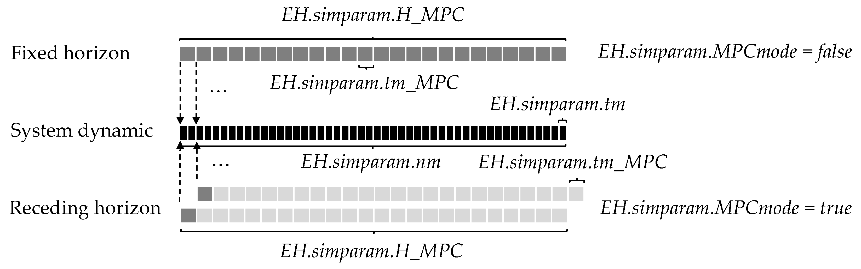
• EH.simparam.nm defines the simulation horizon and, thus, depending on EH.simparam.tm, how many times the loop is executed to obtain the evolution of the system according to its dynamic, that is, updating the state of the storage systems through EH_system.m (which is still in its beta phase).
• EH.simparam.tm defines the time between two consecutive steps of the system’s simulation.
• EH.simparam.tm_MPC defines the time between two consecutive updates of the control action, which is calculated by MPC.m and kept constant at each iteration if EH.simparam.tm_MPC>EH.simparam.tm, and, together with EH.simparam.H_MPC, the number of samples of the model employed for optimization. It cannot be lower than the sample time of the system EH.simparam.tm.
• EH.simparam.H_MPC defines the control horizon, which can be lower than EH.simparam.nm if only the first control action is computed (receding horizon strategy), but needs to be equal to this one for the scheduling mode (fixed horizon strategy). In the first case (MPC mode active), ODEHubs allows also one to apply the variable horizon strategy exemplified in [41].
• EH.simparam.MPCmode determines whether the fixed horizon strategy or the receding horizon strategy is applied. Note that dataEH must contain data for EH.simparam.nm in the first case and for EH.simparam.nm plus EH.simparam.H_MPC in the second one.

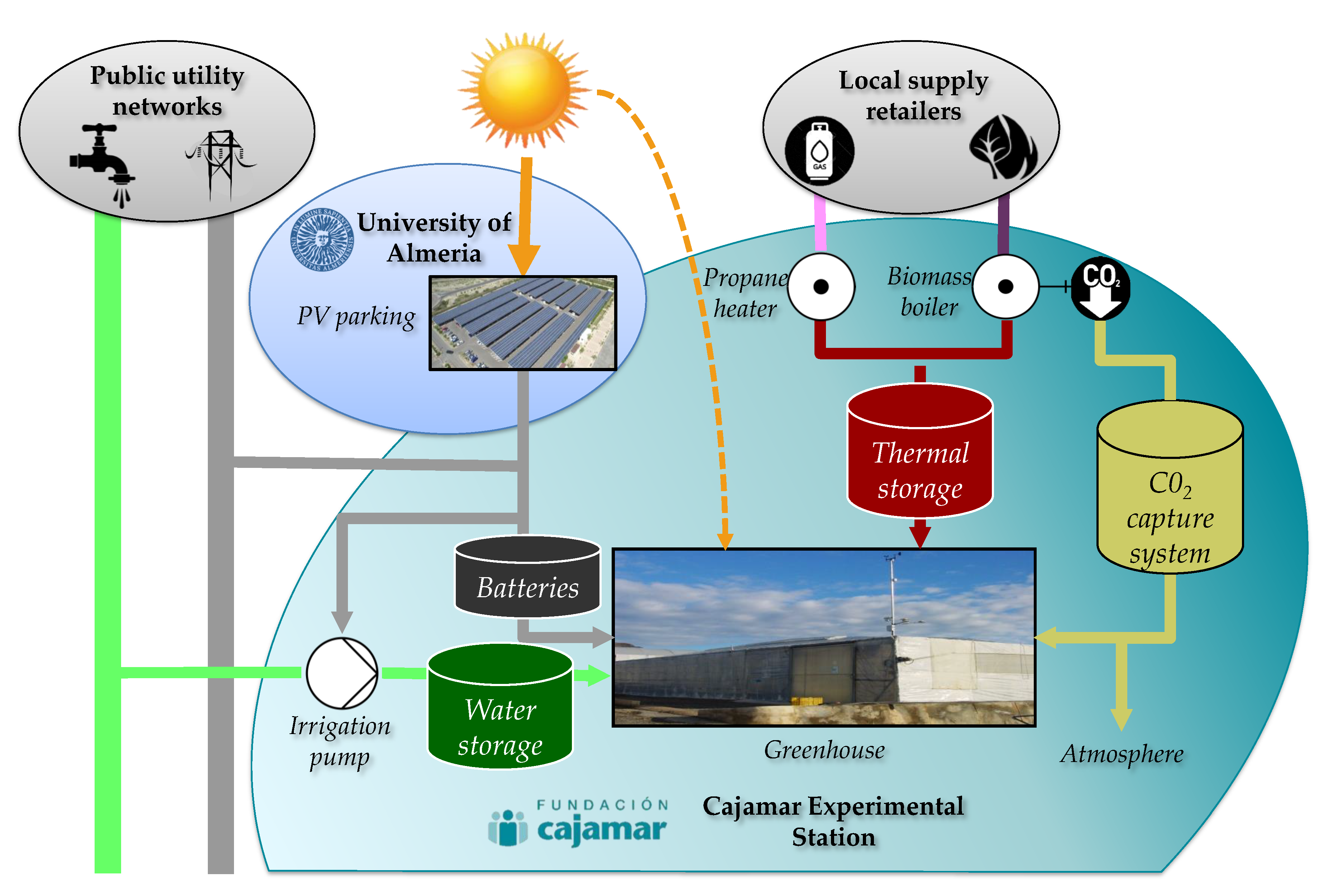
4. Case Study

The EH employed in this how-to section on using ODEHubs consists of two of the plants from he CHROMAE project [21] (Figure 8): the photovoltaic (PV) parking lot placed at the University of Almeria (36.83${}^{\circ }$ N, 2.40${}^{\circ }$ W) and a traditional Mediterranean greenhouse placed at the Experimental Station of the Cajamar Foundation (36.79${}^{\circ }$ N, 2.72${}^{\circ }$ W) [43].

On the one hand, the parral-type greenhouse [44] has a total surface area of 877 m² (37.8 m × 23.2 m), a polyethylene cover, automated ventilation with lateral windows in the northern and southern walls, flap roof windows in each span, and fine-mesh anti-trip nets. The greenhouse orientation is east–west, the crop rows are aligned north–south, and the cropping conditions are very similar to the ones in commercial greenhouses, continuously monitoring several climatic parameters within the greenhouse. Outside, a weather station measures air temperature, relative humidity, solar radiation, liquid precipitations, and wind speed. In addition, the greenhouse has a heating system consisting of a GP 95 propane heater and a Missouri 150,000 multi-fuel boiler, which is part of the CO₂ storage and enrichment system as well [45].

On the other, the photovoltaic parking lot consists of an array of photovoltaic solar panels for production purposes, with 4830 Conergy PA 240P modules connected to 10 Fronius Agilo 100 inverters, and three other arrays for research, connected to their respective Fronius IG Plus 55v3 inverters and distributed as follows: 24 Conergy PA 240P modules in the first one, 24 Conergy Power Plus 240 M modules in the second, and 72 First Solar FS-380 modules in the third. The nominal power of the facility is 1015 kW and the panels are oriented towards the south with a solar azimuth angle of 21${}^{\circ }$ E and a slope of 7${}^{\circ }$.

4.1. Parameters and Modeling

Both facilities are physically separate, but they will be considered a single ensemble that can be modeled by adapting Equations (1)–(16) to the structure represented in Figure 9. In fact, this is automatically done by ODEHubs, which generates the constraints of the optimization problem from the definition given by the users, but they have been included in Appendix A to clarify how the general model is particularized for a specific EHs. In addition, the input parameters required for the toolbox’s blocks are described below before presenting the simulation results from ODEHubs.

Note that in Figure 9, the electric consumption of its 4.5 kW irrigation pump is considered separately from other devices’ consumption in order to match it to the on/off state of the pump. Electricity, as well as the crop needs (water, heat, and CO₂), can be obtained from processing the data acquired by the sensor system of the greenhouse [44], whereas either technical data provided by the manufacturer of each device or one’s own experimental data are employed to define most conversion and storage constraints of the EH. The production model of the photovoltaic parking was obtained by the authors in a former work, considering an isotropic sky model, the equivalent circuit for PV cells, and weather conditions [46]. This allows the determination of the instant availability of solar radiation and, consequently, the setting of the maximum input flow to the field (device 1), which has been scaled to its tenth part in order to analyze a realistic generation–demand situation and the conversion factor (performance) of the same one (

Table 1. Upper and lower limits of conversion, inputs, and market sales flows.

${\mathbf{I}}^{\mathbf{min}}$	${\mathbf{I}}^{\mathbf{max}}$	${\mathbf{M}}^{\mathbf{min}}$	${\mathbf{M}}^{\mathbf{max}}$	${\mathbf{D}}_{\mathbf{i}}^{\mathbf{min}}$	${\mathbf{D}}_{\mathbf{i}}^{\mathbf{max}}$	${\mathbf{D}}_{\mathbf{o}}^{\mathbf{min}}$	${\mathbf{D}}_{\mathbf{o}}^{\mathbf{max}}$
0 kW	∞	0 kW	0 kW	0 kW	[46]	0 kW	∞
0 kW	∞	0 kW	0 kW	0 kW	6.8 kg/h	0 kW	∞
0 kg/h	∞	0 kg/h	∞	1 kg/h	40 kg/h	0 kW	∞
0 kg/h	∞	0 kg/h	0 kg/h	1 kg/h	40 kg/h	0 kg/h	∞
0 m3/h	∞	0 kW	0 kW	0 m3/h	∞	0 m3/h	5 m3/h

and

Table 2. Conversion, degradation, charge, and discharge coefficients.

Coeff.	Value	Coeff.	Value	Coeff.	Value	Coeff.	Value
${\eta }_{D,1}$	[46]	${\eta }_{s,1}$	0.98	${\eta }_{ch,1}$	0.7	${\eta }_{dis,1}$	0.8
${\eta }_{D,2}$	11.54	${\eta }_{s,2}$	0.94	${\eta }_{ch,2}$	0.9	${\eta }_{dis,2}$	0.9
${\eta }_{D,3}$	4.25	${\eta }_{s,3}$	1	${\eta }_{ch,3}$	1	${\eta }_{dis,3}$	1
${\eta }_{D,4}$	1.76	${\eta }_{s,4}$	1	${\eta }_{ch,4}$	1	${\eta }_{dis,4}$	1
${\eta }_{D,5}$	1	${\eta }_{s,5}$	1	${\eta }_{ch,5}$	1	${\eta }_{dis,5}$	1

). Only the water, thermal, and electric storage systems in Figure 9 are hypothetical elements, whose parameters were estimated based on a former study [47].

Once it has finished entering the configuration parameters in the Simulink^® model (Figure 10), ODEHubs will prepare the problem’s setup and get the optimization results, as shown in Figure 2, which includes redefining Equations (1)–(16), as clarified in Appendix A. The parameters that need to be substituted in these equations come from various sources, and they can be classified into time-invariant or variable parameters. Table 1, Table 2 and

Table 3. Storage systems’ upper and lower limits.

${\mathbf{Q}}_{\mathbf{ch}}^{\mathbf{min}}$	${\mathbf{Q}}_{\mathbf{ch}}^{\mathbf{max}}$	${\mathbf{Q}}_{\mathbf{dis}}^{\mathbf{min}}$	${\mathbf{Q}}_{\mathbf{dis}}^{\mathbf{max}}$	${\mathbf{S}}^{\mathbf{min}}$	${\mathbf{S}}^{\mathbf{max}}$
0 kW	3 kW	0 kW	3 kW	0 kWh	11 kWh
0 kW	104.5 kW	0 kW	104.5 kW	0 kWh	116.1 kWh
0 kg/h	51 kg/h	0 kW	51 kg/h	0 kg	25.2 kg
0 m3/h	3 m3/h	0 m3/h	3 m3/h	0 m3	6 m3
0 kW	0 kW	0 kW	0 kW	0 kWh	0 kWh

collect all of them, including their constant values for the first ones and the references of the models employed to periodically get the second ones. Note that the infinite symbol has been employed for unconstrained variables; thereby it is assumed that there is an inexhaustible supply of input resources. The same reasoning applies to the conversion devices, whose upper limits have been defined only for their inputs or for their outputs. There are some elements deliberately missing in Figure 9 ($M_1$, $M_2$, $M_4$, $M_5$, $Q_{ch,5}$, $Q_{dis,5}$, $S_5$), which implies that those flows do not take place in the EH, and the corresponding upper limits are set to zero by ODEHubs (see the fourth column in Table 1 and the fifth row in Table 3).

Regarding the remaining parameters of the model, propane ($c_3=1.694$ EUR/kg), biomass ($c_4=0.255$ EUR/kg), water ($c_5=0.547$ EUR/m³), and electricity prices are obtained from local supply companies. In the case of the electricity ($c_1$), three time periods are distinguished to define the cost: 0.0892 EUR/kWh from 0:00 h to 8:00 h, 0.2044 EUR/kWh from 18:00 h to 22:00 h, and 0.1127 EUR/kWh for the rest of the day. In contrast to the old regulatory framework [41], solar radiation is not taxed ($c_2=0$). Moreover, as the only resource “sold” is the CO₂ freely released to the atmosphere ($M_3$), the price of all the sold resources is null: $\mathit{S}\left(k\right)=\left[\begin{array}{ccccc}0& 0& 0& 0& 0\end{array}\right]$.

Finally, the weather and greenhouse data correspond to the data collected at the said experimental station on 17 December 2018. The choice of that day was made based on the availability of solar radiation (sunny intervals and temperatures between 11 and 21 ${}^{\circ }$C, as shown in Figure 11) and the fact that CO₂ enrichment and heating support were active during part of the day, which results in a scenario where the outputs of the EH have a non-null demand profile (electricity and water are demanded daily, so they are not critical to select the dataset).

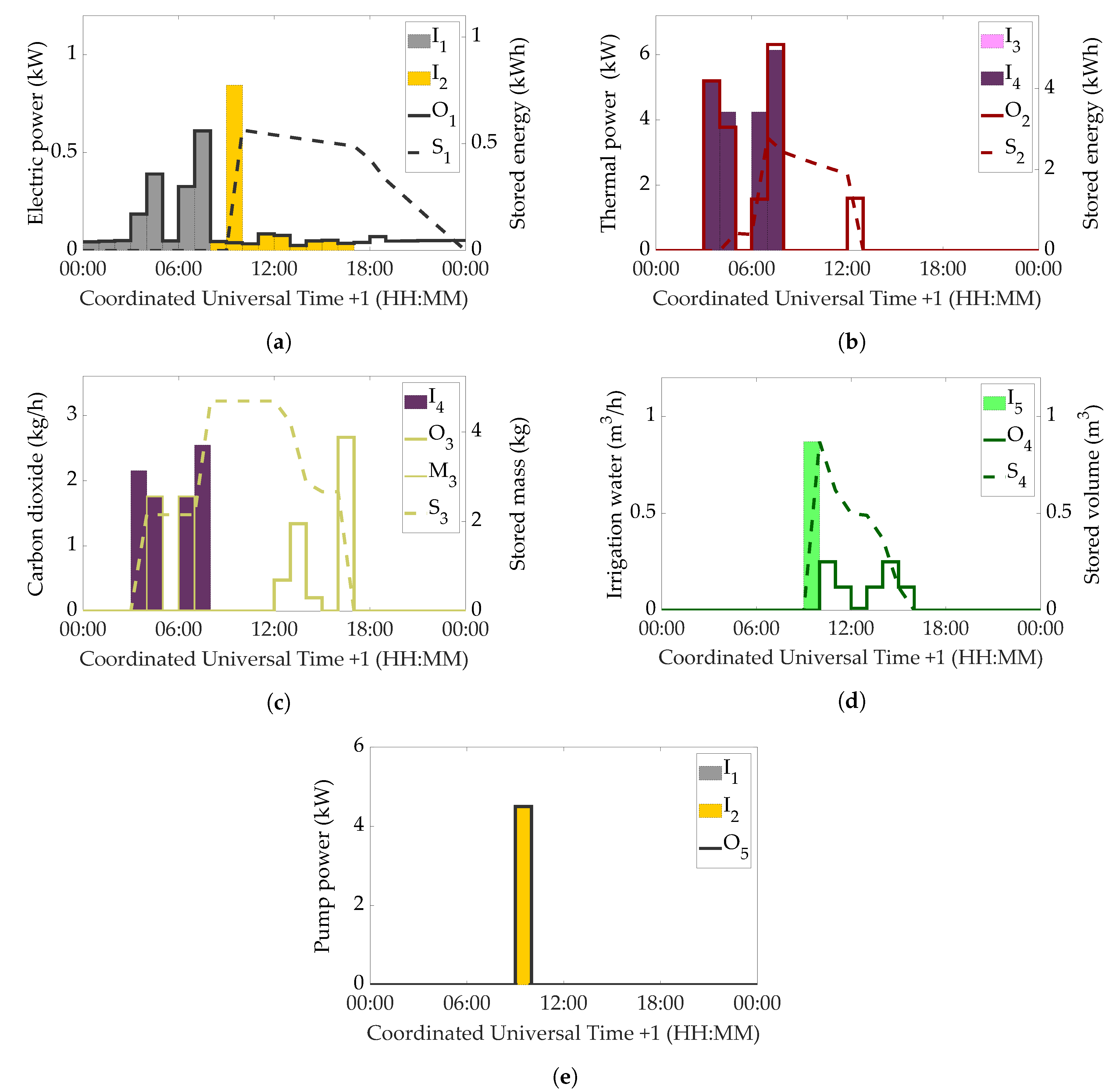
4.2. Simulation Results

The optimal dispatch for the greenhouse was obtained by running ODEHubs with the solver intlinprog [48] and scheduling mode (fixed horizon) on an Intel^® Core^TM i7-6700K 4GHz CPU, taking 0.3219 s to solve the optimization problem. That value means that the tool would probably work as well with shorter sampling times or using MPC mode (receding horizon), which would increase the computational burden. ODEHubs outputs a structure variable that contains all the data defined by the user and post-processed variables, for instance: general parameters of the EH, vectors and matrices of the model, constraints for the solver, and the values of the decision variables.

Although anyone can consult the aforementioned structure, by default, the results are presented in as many graphics as the number of EH’s outputs ($N_o$), arranged in the same way (see Figure 12). Scaled to the left axis and expressed in terms of mass flow, volume flow, or power, the elements of $\mathit{O}$ (demand profiles) are depicted by a thick line together with the elements of $\mathit{M}$, which are stacked over these latter ones and depicted by a thin line. This avoids overlapping between them, as they constitute the left term of Equation (1), which needs to equal the right term, represented with colored stacked bars. These bars actually do not represent any of the variables of the model, but they are obtained from the product of $\mathit{C}$ and $\mathit{P}$ with the purpose of indicating the contribution of each input flow to meeting the demand of resources ($\mathit{O}$). Scaled to the right axis and expressed in terms of mass, volume, or energy, the evolution of the storage systems (elements of $\mathit{S}$) is represented by a dashed line. In this regard, bear in mind that neither the charge (${\mathit{Q}}_{\mathit{C}}$) nor discharge flows (${\mathit{Q}}_{\mathit{D}}$) explicitly appear in the charts, but they can be deducted through either the difference between the bars and the stacked solid lines or the slope of the dashed lines.

By default, ODEHubs sets the upper limit set equal to the maximum capacity of each storage device, but, for the sake of clarity, in this case, they have been customized to show each variable with an appropriate scale. Note that the storage systems are charged whenever the bars are over the stacked solid lines (demand plus sales profiles), or, equivalently, whenever the slope of the dashed line is positive and, by similar reasoning, they are discharged whenever the bars are under the stacked solid lines or the slope is negative. Nonetheless, when analyzing a negative slope, the presence of degradation must be also taken into account, since it has a similar effect. The color choice for each kind of resource is made by the users, and the appearance of the horizontal axis is determined by the sample time, as explained in Section 3.

From Figure 12, which shows the charts of the case study previously presented and the cumulative variables included in ODEHubs’s output structure, the results can be summarized as follows: The 7.02 kWh of electric energy demanded (greenhouse and pump) is covered by purchasing 3.81 kWh from the power grid (0.39 EUR) and the photovoltaic field, which produces energy whenever there is enough solar radiation (see Figure 11); the 18.47 kWh of thermal energy is entirely generated in the biomass boiler because of its lower cost (1.46 EUR) in comparison with propane and its simultaneous use for producing the required 4.69 kg of CO₂; the 0.87 m³ of water (0.48 EUR) is purchased in a single period, between 9:00 and 10:00, in which the availability of solar energy makes up for the slightly higher cost of the electricity at that time (0.1127 versus 0.0892 EUR/kWh at off-peak hours).

5. Conclusions

In view of the results, it can be concluded that ODEHubs is a solid alternative to consider for the formulation and analysis of the dispatch problem in agri-energy hubs, such as that of CHROMAE. Although, for the sake of conciseness, only a specific case study has been evaluated in this paper, it is expected that the tool will be useful in studying resource management strategies with different sets of real data in agro-industrial districts and, because of its conception as a flexible tool, even in industrial, commercial, or home environments. There is still a tradeoff between an accurate representation of some nonlinear processes and the actual formulation as a mixed-integer linear programming problem, which ensures the convergence to a global optimum while keeping the computational burden low. The current solution, however, allows the introduction of variable conversion coefficients, but the constraints could be adapted to consider nonlinear efficiencies due to partial loading [49].

To the best of the authors’ knowledge, many of the control systems proposed in the literature come from the field of chemical engineering, which has traditionally used a hierarchy of levels or layers to distinguish different tasks performed in industry [50]. These are defined attending to the frequency at which decisions are made (i.e., how often the control actions are calculated), the kind and number of equipment involved, or the level of abstraction. Many contributions employ hierarchical control strategies in which an MPC can act in either the regulatory or the supervisory layers as well [51], and, in this regard, there is a dichotomy between Economic MPC and Real-Time Optimization with MPC [52]. Long [40] discusses both approaches in his thesis [40], as well as how the existence of uncertainty affecting the system behavior is sometimes handled by using certainty equivalent model predictive control [53]. From his ideas, one can conclude that, when it comes to certain energy management applications, it is acceptable to assume (a) that the lower-level regulatory controllers have a dynamic fast enough with respect to the sampling interval of the upper layers, and they do not need to be considered for optimization purposes (the corresponding steady states are instead considered), (b) that due to their presence, stability is not a primary concern, and (c) that for demonstration purposes, a general uncertain optimization problem can be converted into a deterministic one. This is the basis of many of the articles found in the literature about energy dispatch that deal with the energetic management of a campus [54] or the energy dispatch of an MG [55], to name a few, and is also the basis of ODEHubs in its current form, whose output corresponds to the computations performed in upper control layers.

Future implementations might incorporate: the interconnection of EHss, which is under development [56], so agents with opposing interests can be considered in the dispatch problem; uncertainty in some of the variables (especially the demanded resources) and arrangement of the consequent probabilistic formulation of the problem; integration of the dispatch problem into the design of facilities, for example, using a bi-level approach in which a genetic algorithm generates possible configurations of the EH [57]; addition of capabilities to incorporate elements from Simscape Simulink^®’s library, which includes components to model different energy networks, such as power grids [58]; or migration of the package to other languages, such as Python or Modelica^®. Python programs are executed from a command line, similarly to MATLAB^® scripts from the command prompt, and there are already some tools built in that language [25], and Modelica^® is an object-oriented modeling language that has already been used to implement models of some of the components of the CHROMAE project [59].

References

1. Mohammadi, M.; Noorollahi, Y.; Mohammadi-ivatloo, B.; Yousefi, H. Energy hub: From a model to a concept—A review. Renew. Sustain. Energy Rev. 2017, 80, 1512–1527. [Google Scholar] [CrossRef]
2. Ehsan, A.; Yang, Q. Optimal integration and planning of renewable distributed generation in the power distribution networks: A review of analytical techniques. Appl. Energy 2018, 210, 44–59. [Google Scholar] [CrossRef]
3. Chicco, G.; Mancarella, P. Distributed multi-generation: A comprehensive view. Renew. Sustain. Energy Rev. 2009, 13, 535–551. [Google Scholar] [CrossRef]
4. Geidl, M.; Koeppel, G.; Favre-Perrod, P.; Klöckl, B.; Andersson, G.; Fröhlich, K. Energy hubs for the future. IEEE Power Energy Mag. 2006, 5, 24–30. [Google Scholar] [CrossRef]
5. Geidl, M.; Andersson, G. Optimal power flow of multiple energy carriers. IEEE Trans. Power Syst. 2007, 22, 145–155. [Google Scholar] [CrossRef]
6. Sadeghi, H.; Rashidinejad, M.; Moeini-Aghtaie, M.; Abdollahi, A. The energy hub: An extensive survey on the state-of-the-art. Appl. Therm. Eng. 2019, 161, 114071. [Google Scholar] [CrossRef]
7. Maroufmashat, A.; Taqvi, S.T.; Miragha, A.; Fowler, M.; Elkamel, A. Modeling and optimization of energy hubs: A comprehensive review. Inventions 2019, 4, 50. [Google Scholar] [CrossRef] [Green Version]
8. Mancarella, P. MES (multi-energy systems): An overview of concepts and evaluation models. Energy 2014, 65, 1–17. [Google Scholar] [CrossRef]
9. Farah, A.; Hassan, H.; Abdelshafy, M.A.; Mohamed, M.A. Optimal scheduling of hybrid multi-carrier system feeding electrical/thermal load based on particle swarm algorithm. Sustainability 2020, 12, 4701. [Google Scholar] [CrossRef]
10. Konneh, D.; Howlader, H.; Shigenobu, R.; Senjyu, T.; Chakraborty, S.; Krishna, N. A multi-criteria decision maker for grid-connected hybrid renewable energy systems selection using multi-objective particle swarm optimization. Sustainability 2019, 11, 1188. [Google Scholar] [CrossRef] [Green Version]
11. Menezes Morato, M.; da Costa Mendes, P.R.; Normey-Rico, J.E.; Bordons, C. Optimal operation of hybrid power systems including renewable sources in the sugar cane industry. IET Renew. Power Gener. 2017, 11, 1237–1245. [Google Scholar] [CrossRef]
12. Galvan, E.; Mandal, P.; Chakraborty, S.; Senjyu, T. Efficient energy-management system using a hybrid transactive-model predictive control mechanism for prosumer-centric networked microgrids. Sustainability 2019, 11, 5436. [Google Scholar] [CrossRef] [Green Version]
13. Bordons, C.; Garcia-Torres, F.; Ridao, M.Á. Model predictive control of interconnected microgrids and electric vehicles. Rev. Iberoam. Autom. Inform. Ind. 2020, 17, 239–253. [Google Scholar] [CrossRef]
14. Gil, J.D.; Roca, L.; Berenguel, M. Modeling and automatic control in solar membrane distillation: Fundamentals and proposals for its technological development. Rev. Iberoam. Autom. Inform. Ind. 2020, 17, 329–342. [Google Scholar] [CrossRef]
15. Nawalany, G.; Sokołowski, P. Improved energy management in an intermittently heated building using a large broiler house in central Europe as an example. Energies 2020, 13, 1371. [Google Scholar] [CrossRef] [Green Version]
16. Shen, Y.; Wei, R.; Xu, L. Energy consumption prediction of a greenhouse and optimization of daily average temperature. Energies 2018, 11, 65. [Google Scholar] [CrossRef] [Green Version]
17. Van Beveren, P.J.M.; Bontsema, J.; van Straten, G.; van Henten, E.J. Optimal utilization of a boiler, combined heat and power installation, and heat buffers in horticultural greenhouses. Comput. Electron. Agric. 2019, 162, 1035–1048. [Google Scholar] [CrossRef]
18. Ouammi, A.; Achour, Y.; Dagdougui, H.; Zejli, D. Optimal operation scheduling for a smart greenhouse integrated microgrid. Energy Sustain. Dev. 2020, 58, 129–137. [Google Scholar] [CrossRef]
19. Muñoz, M.; Gil, J.D.; Roca, L.; Rodríguez, F.; Berenguel, M. An IoT architecture for water resource management in agroindustrial environments: A case study in Almería (Spain). Sensors 2020, 20, 596. [Google Scholar] [CrossRef] [Green Version]
20. Mérida García, A.; Fernández García, I.; Camacho Poyato, E.; Montesinos Barrios, P.; Rodríguez Díaz, J.A. Coupling irrigation scheduling with solar energy production in a smart irrigation management system. J. Clean. Prod. 2018, 175, 670–682. [Google Scholar] [CrossRef]
21. ARM-TEP197. CHROMAE Project (DPI2017-85007-R). 2017. Available online: http://www2.ual.es/chromae/ (accessed on 1 September 2020).
22. Web Site of the ARM Group. Automatic Control, Robotics, and Mechatronics (ARM) Research Group (TEP-197). 2020. Available online: https://arm.ual.es/arm-group/ (accessed on 1 August 2020).
23. Allegrini, J.; Orehounig, K.; Mavromatidis, G.; Ruesch, F.; Dorer, V.; Evins, R. A review of modeling approaches and tools for the simulation of district-scale energy systems. Renew. Sustain. Energy Rev. 2015, 52, 1391–1404. [Google Scholar] [CrossRef]
24. Van Beuzekom, I.; Gibescu, M.; Slootweg, J. A review of multi-energy system planning and optimization tools for sustainable urban development. In Proceedings of the 2015 IEEE Eindhoven PowerTech, Eindhoven, The Netherlands, 29 June–2 July 2015; pp. 1–7. [Google Scholar] [CrossRef]
25. Groissböck, M. Are open source energy system optimization tools mature enough for serious use? Renew. Sustain. Energy Rev. 2019, 102, 234–248. [Google Scholar] [CrossRef]
26. Ringkjøb, H.K.; Haugan, P.M.; Solbrekke, I.M. A review of modeling tools for energy and electricity systems with large shares of variable renewables. Renew. Sustain. Energy Rev. 2018, 96, 440–459. [Google Scholar] [CrossRef]
27. International Business Machines Corporation (IBM). IBM ILOG CPLEX Optimization Studio. 2019. Available online: https://www.ibm.com/es-es/products/ilog-cplex-optimization-studio (accessed on 1 September 2020).
28. Bisschop, J.; Meeraus, A. On the development of a general algebraic modeling system in a strategic planning environment. In Applications; Mathematical Programming Studies; Springer: Heidelberg/Berlin, Germany, 1982; Volume 20, pp. 1–29. [Google Scholar]
29. Fourer, R.; Gay, D.M.; Kernighan, B. AMPL: A mathematical programming language. In Algorithms and Model Formulations in Mathematical Programming; Wallace, S.W., Ed.; Springer: Berlin/Heidelberg, Germany, 1989; pp. 150–151. [Google Scholar]
30. Bisschop, J. AIMMS–Optimization Modeling; Paragon Decision Technology B.V: Haarlem, The Netherlands, 2006. [Google Scholar]
31. The MathWorks, Inc. MATLAB R2020a. 2020. Available online: http://es.mathworks.com/products/matlab/ (accessed on 1 August 2020).
32. R Core Team. R: A Language and Environment for Statistical Computing; R Foundation for Statistical Computing: Vienna, Austria, 2013. [Google Scholar]
33. Van Rossum, G.; Drake, F.L., Jr. Python Reference Manual; Centrum voor Wiskunde en Informatica: Amsterdam, The Netherlands, 1995. [Google Scholar]
34. Bollinger, L.A.; Dorer, V. The Ehub Modeling Tool: A flexible software package for district energy system optimization. Energy Procedia 2017, 122, 541–546. [Google Scholar] [CrossRef]
35. Darivianakis, G.; Georghiou, A.; Smith, R.S.; Lygeros, J. EHCM Toolbox. 2015. Available online: https://people.ee.ethz.ch/~building/ehcmToolbox/EHCM_Documentation.pdf (accessed on 1 August 2020).
36. Zimmerman, R.D.; Murillo-Sánchez, C.E. Matpower Optimal Scheduling Tool (MOST) User’s Manual, Version 1.0.2. 2019. Available online: https://github.com/MATPOWER/most/blob/master/docs/MOST-manual.pdf (accessed on 1 August 2020).
37. Kühne, M.R. Drivers of Energy Storage Demand in the German Power System: An Analysis of the Influence of Methodology and Parameters on Modeling Results. Ph.D. Thesis, Technical University of Munich, Munich, Germany, 2016. [Google Scholar]
38. Van den Bergh, K.; Bruninx, K.; Delarue, E.; D’haeseleer, W. LUSYM: A Unit Commitment Model Formulated as a Mixed-Integer Linear Program; KU Leuven Energy Institute, TME Branch Energy Environment: Leuven, Germany, 2014; Volume 7. [Google Scholar]
39. Brancucci Martinez-Anido, C. Electricity without Borders—The Need for Cross-Border Transmission Investment in Europe. Ph.D. Thesis, Delft University of Technology, Delft, The Netherlands, 2013. [Google Scholar]
40. Long, S. Generalized Modeling Framework for Multi-Energy Systems with Model Predictive Control Applications. Ph.D. Thesis, University of Manchester, Manchester, UK, 2019. [Google Scholar]
41. Ramos-Teodoro, J.; Rodríguez, F.; Berenguel, M.; Torres, J.L. Heterogeneous resource management in energy hubs with self-consumption: Contributions and application example. Appl. Energy 2018, 229, 537–550. [Google Scholar] [CrossRef] [Green Version]
42. Löfberg, J. YALMIP: A toolbox for modeling and optimization in MATLAB. In Proceedings of the 2004 IEEE International Conference on Robotics and Automation, New Orleans, LA, USA, 2–4 September 2004; pp. 284–289. [Google Scholar] [CrossRef]
43. Foundation, C. Cajamar Experimental Station. 2020. Available online: https://www.fundacioncajamar.es/es/comun/estacion-experimental-palmerillas/ (accessed on 1 September 2020).
44. Sánchez-Molina, J.A.; Rodríguez, F.; Guzmán, J.L.; Arahal, M.R. Virtual sensors for designing irrigation controllers in greenhouses. Sensors 2012, 12, 15244–15266. [Google Scholar] [CrossRef] [Green Version]
45. Sánchez-Molina, J.A.; Reinoso, J.V.; Acién, F.G.; Rodríguez, F.; López, J.C. Development of a biomass-based system for nocturnal temperature and diurnal CO2 concentration control in greenhouses. Biomass Bioenergy 2014, 67, 60–71. [Google Scholar] [CrossRef]
46. Ramos-Teodoro, J.; Rodríguez, F.; Berenguel, M. Photovoltaic facilities modeling for an energy hub management with heterogeneous resources. In Proceedings of the XVI CEA Symposium on Control Engineering, Almeria, Spain, 7–9 March 2018; pp. 23–30. (In Spanish). [Google Scholar]
47. Ramos-Teodoro, J. Energy Management of a Heterogeneous Production System under the Energy Hub Paradigm. Master’s Thesis, Department of Systems Engineering and Automation, University Carlos III of Madrid, Madrid, Spain, 2017. (In Spanish). [Google Scholar]
48. The MathWorks Inc. Documentation: Intlinprog. Available online: https://es.mathworks.com/help/optim/ug/intlinprog.html (accessed on 1 September 2020).
49. Evins, R.; Orehounig, K.; Dorer, V.; Carmeliet, J. New formulations of the ‘energy hub’ model to address operational constraints. Energy 2014, 73, 387–398. [Google Scholar] [CrossRef]
50. am Ende, D.J.; am Ende, M.T. Chemical Engineering in the Pharmaceutical Industry: Drug Product Design, Development, and Modeling; John Wiley & Sons: Hoboken, NJ, USA, 2019; p. 567. [Google Scholar]
51. Aydın, E.; Arkun, Y.; Is, G. Economic model predictive control (EMPC) of an industrial diesel hydroprocessing plant. IFAC-PapersOnLine 2016, 49, 568–573. [Google Scholar] [CrossRef]
52. Tran, T.; Ling, K.; Maciejowski, J.M. Economic model predictive control—A review. In Proceedings of the 31st International Symposium on Automation and Robotics in Construction, Sydney, Australia, 9–11 July 2014; Volume 31, p. 1. [Google Scholar]
53. Skaf, J.; Boyd, S.P. Design of affine controllers via convex optimization. IEEE Trans. Autom. Control 2010, 55, 2476–2487. [Google Scholar] [CrossRef] [Green Version]
54. Long, S.; Marjanovic, O.; Parisio, A. Generalized control-oriented modeling framework for multi-energy systems. Appl. Energy 2019, 235, 320–331. [Google Scholar] [CrossRef] [Green Version]
55. Nassourou, M.; Blesa, J.; Puig, V. Optimal energy dispatch in a smart micro-grid system using economic model predictive control. Proc. Inst. Mech. Eng. Part I J. Syst. Control Eng. 2020, 234, 96–106. [Google Scholar] [CrossRef] [Green Version]
56. Ramos-Teodoro, J.; Rodríguez, F.; Castilla, M.; Berenguel, M. Modeling of production, consumption and storage of heterogeneous resources of a agri-food district with renewable energies. In Proceedings of the X Iberian Congress on Agro-Engineering, Huesca, Spain, 3–6 September 2019; pp. 190–198. (In Spanish) [Google Scholar] [CrossRef]
57. Evins, R. Multi-level optimization of building design, energy system sizing and operation. Energy 2015, 90, 1775–1789. [Google Scholar] [CrossRef]
58. Montoya, O.D.; Gil-González, W.; Avila-Becerril, S.; Garces, A.; Espinosa-Pérez, G. Distributed energy resources integration in AC grids: A family of passivity-based controllers. Rev. Iberoam. Autom. Inform. 2019, 16, 212–221. (In Spanish) [Google Scholar] [CrossRef]
59. Gómez, F.J.; Yebra, L.J.; Giménez, A.; Torres-Moreno, J.L. Modeling of batteries for application in light electric urban vehicles. Rev. Iberoam. Autom. Inform. Ind. 2019, 16, 459–466. (In Spanish) [Google Scholar] [CrossRef]
Figure 1. Example energy hub (EH) where the electric pump ( D 1 ) works at any time there exists a flow between the public supply network ( I 1 ) and the water demand ( O 1 ) or the storage tank ( Q c h , 1 ). I 2 represents the electricity from the power grid that covers the pump’s demand ( O 2 ).
Sustainability 12 08820 g001
Figure 2. Flowchart of the Optimal Dispatch for Energy Hubs (ODEHubs) library that shows the processes involved in defining and simulating an EH and the main files or folders related to them (in italics).
Sustainability 12 08820 g002
Figure 3. ODEHubs’s library components defined in Simulink®, which can be used to define customized systems either by including their elements in Simulink’s browser or by copying them from the library file. The name that appears under each block can be changed when the block is included in a Simulink® model, as well as the labels within Input and Output blocks.
Sustainability 12 08820 g003
Figure 4. Parameters of the Input (a) and Output (b) blocks in Simulink®.
Sustainability 12 08820 g004
Figure 5. Parameters of the Convergence Node (a) and Divergence Node (b) blocks in Simulink®.
Sustainability 12 08820 g005
Figure 6. Parameters of the Storage System (a) and device blocks (b) in Simulink®.
Sustainability 12 08820 g006
Figure 7. Interpretation of the configuration parameters related to sample time and horizon for the system and the control layer depending on the selected mode. The dashed arrows indicate when the control action is updated, and the dark gray squares indicate which control actions are computed.
Sustainability 12 08820 g007
Figure 8. Functional diagram of the EH analyzed in the case study. The greenhouse demands thermal and electric energy, water, and CO2 for crop growth, which are supplied either directly from the public utility networks or after transforming other input resources in the facilities of the plant. Several storage systems serve as backups to compensate variations in the demands.
Sustainability 12 08820 g008
Figure 9. Particularization of the general conversion and storage model for the plant, where the irrigation pump ( D 4 ) works at any time there exists a flow between the public supply network ( I 5 ) and the water demand ( O 4 ) or the storage tank ( Q c h , 4 ). I 1 represents the electricity from the power grid and I 2 represents the solar power, and they cover both the greenhouse’s ( O 1 ) and the pump’s ( O 5 ) demands. Propane ( I 3 ) and biomass ( I 4 ) are other input resources used to produce the thermal power ( O 2 ) and CO2 ( O 3 ) required by the crops. M 3 expresses the amount of CO2 released from storage due to lack of capacity.
Sustainability 12 08820 g009
Figure 10. Case study EH defined through ODEHubs’s blocks in Simulink®. The labels within some blocks are customizable for representation purposes, although by default, ODEHubs names each input and output to present the results according to the number between parentheses, matching the notation in Figure 9. ODEHubs also renames the Storage system blocks according to the label of the Output block to which they are connected. In this diagram, the labels within Input and Output blocks and the name of each device have been chosen to identify the kind of resources and device, but they are related to Figure 9 as follows. Devices: D 1 → PVpk (photovoltaic parking lot), D 2 → PBgh (propane heater), D 3 → BBgh (biomass boiler), D 4 → IPgh (irrigation pump). Inputs: I 1 → Ei, I 2 → Rpk, I 3 → Pi, I 4 → Bi, I 5 → Wi. Outputs: O 1 → Eo, O 2 → Hgh, O 3 → Go, O 4 → Wo, O 5 → Esgh. Note that M 3 is missing because the block Go has been configured to allow sale of the resources attached to that output (see Figure 4b).
Sustainability 12 08820 g010
Figure 11. Weather conditions on 17 December 2018. Apart from global horizontal irradiance (GHI), direct normal irradiance (DNI) and diffuse horizontal irradiance (DHI) determine the amount of power produced by the photovoltaic field, and temperature (a) allows the estimation of the performance of the cells. DNI requires a different scale (a), with respect to GHI and DHI (b), owing to the direction of the normal beam of radiation, which results in higher values of the irradiance around midday. As data are recorded every minute, ODEHubs calculates the hourly average to simulate the case study.
Sustainability 12 08820 g011
Figure 12. Optimal economic dispatch of resources in the greenhouse on 17 December 2018, obtained with ODEHubs. The demands (O) are represented by solid thick lines, the bars indicate the contribution of each input (I), and the evolution of the storage systems (S) is represented by dashed thick lines, all arranged according to the output variables as indicated between parentheses: O1 (a), O2 (b), O3 (c), O4 (d), O5 (e).
Sustainability 12 08820 g012