Article

Analysis of Multi-Objective Optimization of Machining Allowance Distribution and Parameters for Energy Saving Strategy

1
School of Intelligence and Technology, National University of Defense Technology, Changsha 410073, China
2
Industrial Engineering Center, Zhejiang Province Key Laboratory of Advanced Manufacturing Technology, Zhejiang University, Hangzhou 310058, China
*
Author to whom correspondence should be addressed.
Sustainability 2020, 12(2), 638; https://doi.org/10.3390/su12020638
Submission received: 7 December 2019 / Revised: 8 January 2020 / Accepted: 13 January 2020 / Published: 15 January 2020

Abstract

:
Machining allowance distribution and related parameter optimization of machining processes have been well-discussed. However, for energy saving purposes, the optimization priorities of different machining phases should be different. There are often significant incoherencies between the existing research and real applications. This paper presents an improved method to optimize machining allowance distribution and parameters comprehensively, considering energy-saving strategy and other multi-objectives of different phases. The empirical parametric models of different machining phases were established, with the allowance distribution problem properly addressed. Based on previous analysis work of algorithm performance, non-dominated sorting genetic algorithm II and multi-objective evolutionary algorithm based on decomposition were chosen to obtain Pareto solutions. Algorithm performances were compared based on the efficiency of finding the Pareto fronts. Two case studies of a cylindrical turning and a face milling were carried out. Results demonstrate that the proposed method is effective in trading-off and finding precise application scopes of machining allowances and parameters used in real production. Cutting tool life and surface roughness can be greatly improved for turning. Energy consumption of rough milling can be greatly reduced to around 20% of traditional methods. The optimum algorithm of each case is also recognized. The proposed method can be easily extended to other machining scenarios and can be used as guidance of process planning for meeting various engineering demands.

1. Introduction

Despite the increasing use of low carbon energy sources, fossil fuels remain as the dominant energy sources worldwide [1,2], with their share accounting for 81% in 2008 to 74% in 2035 [3,4]. The rising demand for fossil fuels led to CO2 emissions rising from 29.3 gigatons (Gt) in 2008 to 35.4 Gt in 2035 [5,6]. Researchers suggested that the widely-used machining processes are responsible for about 84 percent of energy-related CO2 emissions and 90 percent of the energy consumption in the industrial sector [7,8,9]. Therefore, reasonable planning of the machining process can be effective in improving the energy consumption and carbon emission situation [10]. Energy savings up to 6%–40% can be obtained based on the optimum choice of cutting parameters and machining allowance distribution [11].
While in real production, the optimization focus varies with different phases of the process. During rough machining, the equilibrium between production rate and energy consumption will be the main consideration. However, the quality of the products is the priority during finish machining.
In this research, for the comprehensive optimization of production quality, efficiency and energy-saving, a method to optimize the machining planning strategy of the whole process is presented. Modeling of optimization objectives on each phase was carried out, including steps of theoretical analysis, experiment, and statistical regression. The optimum machining allowance and parameters of different phases were obtained, which is based on the principle of finding Pareto fronts for multi-objective optimization.
Outer cylinder turning and face milling were carried out as case studies. It is revealed that the proposed method is effective in finding the equilibrium between low-carbon manufacturing and production demand fulfillment. The overall flow of this research is shown in Figure 1.
The remainder of this paper is organized as follows. The literature review is presented in the next section. Detailed discussions of the modeling method for machining allowance distribution and multi-objective optimizations are given in section “Modeling of machining process considering machining allowance distribution”, followed by case studies to verify the proposed method in section “Case studies”. Finally, the conclusion and future research directions are summarized in section “Conclusion and future work”.

2. Literature Review

Reasonable planning of the machining process, which includes optimization of machining parameters and machining allowance distribution, etc., can be effective in improving the energy consumption and carbon emission situation.
Therefore, many researchers have highlighted the optimization of machining parameters. For example, Lv et al. [12] carried out an investigation into methods for predicting material removal energy consumption in turning. Jia et al. [13] established prediction models for feeding power and material drilling power to support sustainable machining. Franco et al. [14] analyzed a parametric model of energy consumption in micro-drilling processes. Sealy [15] proposed a new parametric energy consumption model with high accuracy in precision hard milling for sustainability.
While research of merely modeling or single-objective optimizations has limits in trading-off., machining parameters implicated by sustainability requirements should not give way to deteriorations affecting quality and productivity [16,17].
Therefore, many of the existing works are multi-objective optimization problems (MOP), considering the equilibrium between energy saving and economic objectives. For example, Li et al. [18] carried out selection of optimum parameters in multi-pass face milling for maximum energy efficiency and minimum production cost. Albertelli et al. [19] presented an energy-oriented multi cutting parameter optimization in face milling. Wang et al. [20] carried out multi-objective optimization considering energy consumption, cost, and surface roughness for a turning process. Yan and Li [21] proposed a multi-objective optimization method called RSM in the milling process, which is to evaluate trade-offs between sustainability, production rate, and cutting quality.
However, these studies ignored the fact that, in real production, optimization focus varies in accordance with different phases of processes. The machining allowance distribution of each phase should also be taken into consideration.
Machining allowance is the workpiece provided beyond the finished contours on a prepared component, which is subsequently removed in machining. There are two machining allowances for each of the process phases, which typically include the rough machining and the finish machining. The machining allowance distribution of each phase can be crucial in meeting the demands in real production, and related machining parameter optimization of each phase should also be taken into consideration comprehensively.
However, during the rough machining phase, the machining process mainly focuses on process efficiency in real production. For example, Camposeco-Negrete [22] presented an experimental study to optimize machining time under roughing conditions. On the other hand, however, the finish machining phase mainly focuses on quality demands. For example, Wei et al. [23] carried out a prediction of cutting force of ball-end milling for high efficiency, precision, and equipment utilization. Hanafi et al. [24] determined the optimal setting of machining parameters in terms of minimum surface roughness and cutting power.
These studies barely consider the comprehensive distribution of machining allowance to find the equilibrium of different phases, and the energy consumption issues were ignored or incompletely involved in reducing carbon emission.
For the machining allowance analysis, Zhang et al. [25] proposed a force-measuring-based approach for feed rate optimization considering the machining allowance. Jiang et al. [26] proposed a non-uniform allowance allocation method for NC programming of structural parts.
However, these studies either barely focus on energy consumption, or dwell on the system-level, which implies that the optimization results will have little value in improving the process in detail. Actually, according to our investigation, the existing studies about machining allowance distribution rarely concern process improvement for energy saving so far.
In summary, machining allowance distribution and parameter optimization for energy-saving strategies deserve further study.

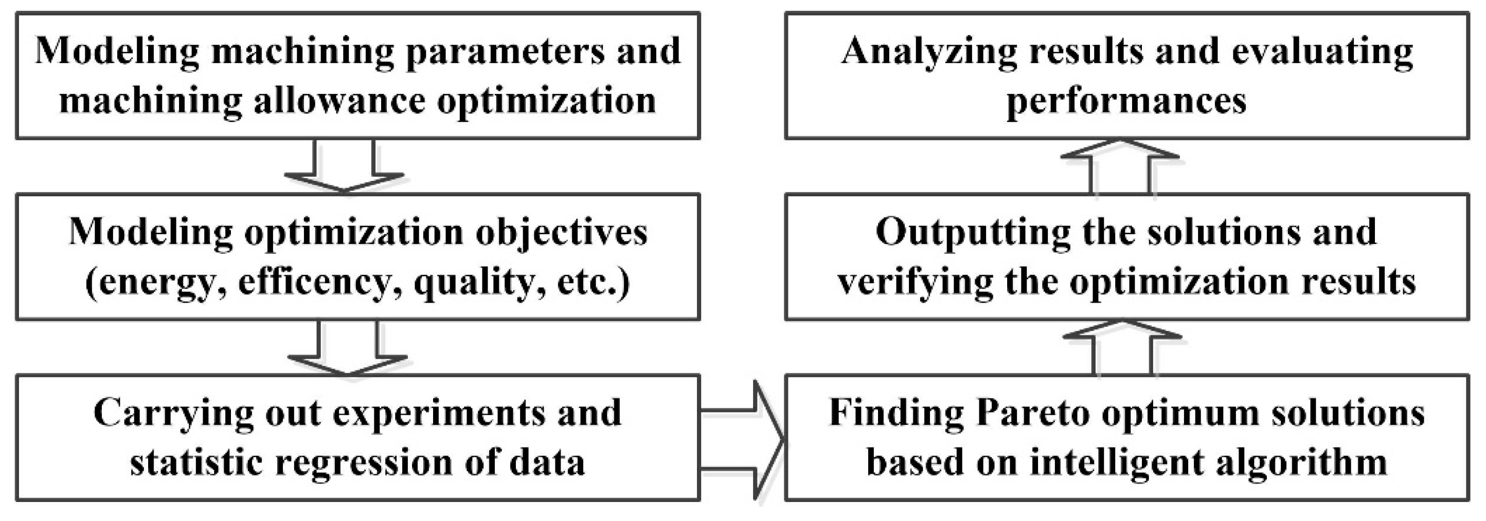
3. Modeling of Machining Process Considering Machining Allowance Distribution

In this research, the most commonly used machining processes of cylindrical turning and step milling are used as case studies for deliberating the problem. The analysis of the two kinds can be used as guidance for future applications in other complex scenarios.

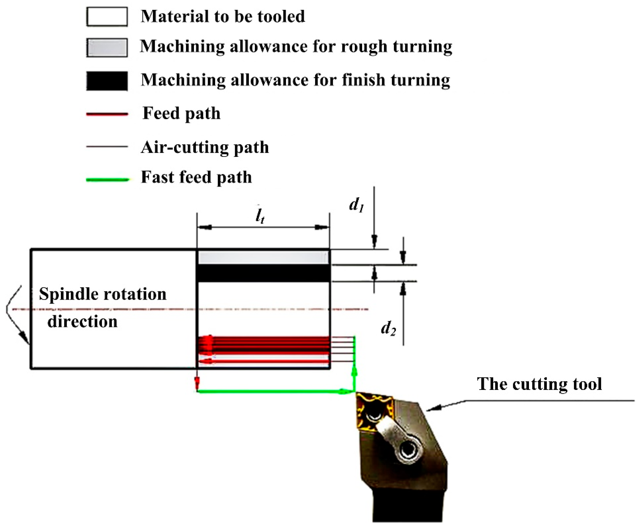
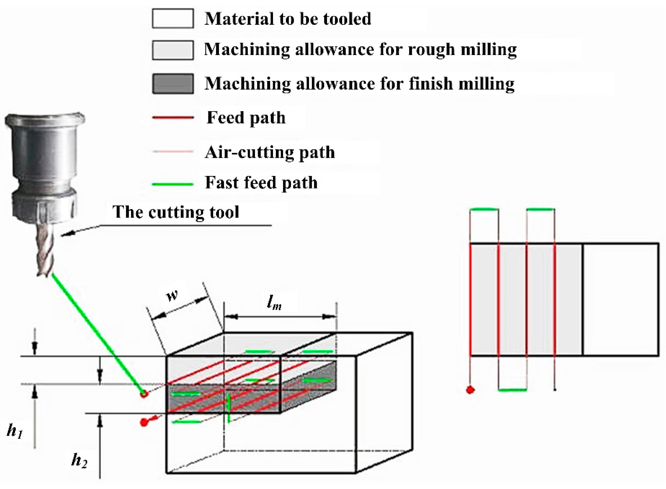
3.1. Optimization Focuses During Different Machining Phases

When the total volume to be tooled is fixed, the allowance distribution of different machining phases can be crucial to meet the production demands. Figure 2 shows the machining allowance distribution of a typical cylindrical turning process with rough turning and finish turning. l t is the total axial length of the workpiece to be tooled. d 1 and d 2 are the radial distance of the workpiece for rough turning and finish turning, and they are taken as the machining allowances of the two turning phases.
Therefore, the total material volume to be tooled in a turning process V t can be expressed as Equation (1). R is the radius of the original cylindrical workpiece.
V t = l t · π · [ R 2 ( R d 1 d 2 ) 2 ]
During different phases of the turning process, machining parameter groups can be different. During rough turning, the cutting parameters include cutting speed v rt [ m / min ] , spindle rotation speed n rt   [ rpm ] , feed rate f rt [ mm / rec ] , feed speed f vrt [ mm / min ] , cutting depth a prt [ mm ] , and during finish turning, those include cutting speed v ft [ m / min ] , spindle rotation speed n ft [ rpm ] , feed rate f ft [ mm / r ] , feed speed f vft [ mm / min ] , cutting depth a pft [ mm ] , respectively.
The optimization focus of these parameters depends on different optimization objectives of each phase. During rough turning, the optimization objectives include reducing energy consumption E rt [ J ] for low-carbon emission, minimizing feeding time t frt [ min ] for production efficiency. Besides, because of the relatively big cutting parameters causing damage to cutting tools, the cutting tool life TL rt [ min ] should also be taken into consideration. On the other hand, the optimization objectives of finish turning phase include reducing energy consumption E ft [ J ] , minimizing feeding time t fft [ min ] for production efficiency, minimizing surface roughness R at [ μ m ] for quality assurance, and because of the frequently used high-speed cutting during finish turning, the cutting tool life during finish turning TL ft [ min ] should also be considered.
Similarly, Figure 3 shows the machining allowance distribution of a typical step milling process. l m [ mm ] is the length of the workpiece to be tooled, w [ mm ] is the width, h 1 [ mm ] and h 2 [ mm ] are heights of the workpiece for rough milling and finish milling. Therefore, the total workpiece volume to be tooled in a milling process V m can be expressed as Equation (2):
V m = l m · w · ( h 1 + h 2 )
During rough milling, machining parameters include cutting speed v rm [ m / min ] , spindle rotation speed n rm [ rpm ] , feed rate f rm [ mm / rec ] , feed speed f vrm [ mm / min ] , cutting depth a prm [ mm ] , cutting width a erm [ mm ] , and for finish milling, those include cutting speed v fm [ m / min ] , spindle rotation speed n rm [ rpm ] , feed rate f fm [ mm / rec ] , feed speed f vrm [ mm / min ] , cutting depth a pfm [ mm ] , and cutting width a efm [ mm ] .
Similarly, the optimization objectives of rough milling include reducing energy consumption E rm [ J ] for low-carbon emission, minimizing cutting time t frm [ min ] for production efficiency, and extending cutting tool life TL rm [ min ] , and for finish turning, those include reducing energy consumption E fm [ J ] , minimizing cutting time t ffm [ min ] , minimizing surface roughness R am [ μ m ] for quality assurance, and extending cutting tool life during finish turning TL fm [ min ] .
The information about cutting parameters, optimization objectives and machining allowance distribution for both turning and milling processes are listed in Table 1 as follows.

3.2. Modeling of Relation between Cutting Parameters and Optimization Objectives

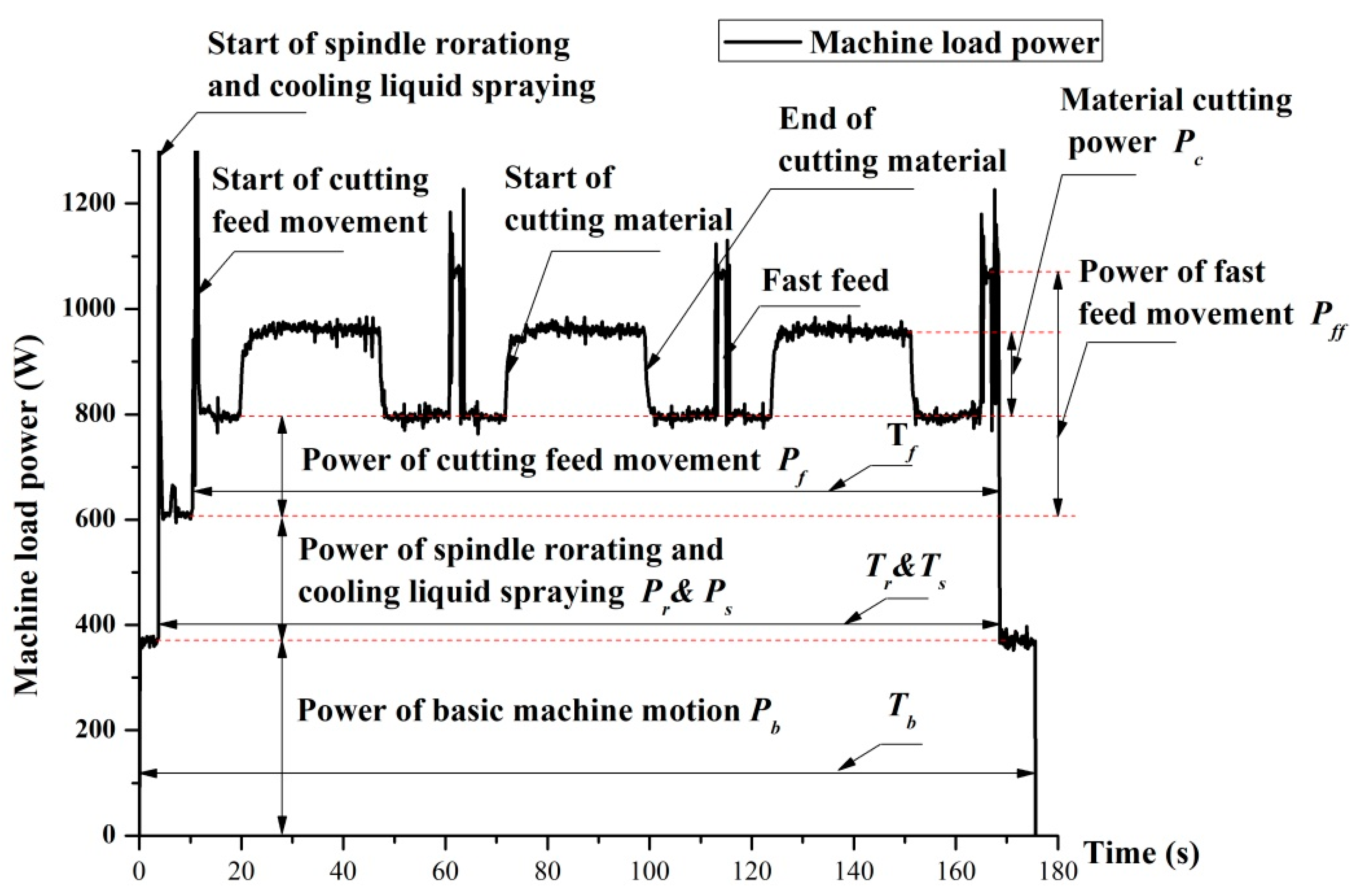
3.2.1. Modeling of Energy Consumption During Machining Process

According to our previous work [27,28], the energy consumption objective E o during a machining process with a fixed group of machining parameters can be approximately expressed as Equation (3). t f is the lasting time of feed movement, t c is the lasting time of cutting materials. Figure 4 shows the power profile of a typical milling process:
E o = ( P b + P s + P r + P f ) t f + P c t c .
By carrying out experiments, the values of basic machine motion power P b and fluid spraying power P s can be directly measured [27]. The selection of parameters, set-up, data acquisition, and analysis methods of the experiments can be found in our previous work [29,30], and Figure 5 shows the diagram of the experimental set-up.
There is a piecewise relation between the spindle rotation power P r and spindle speed n   [ r / min ] . This can be expressed as a piecewise function as Equation (4), where   C rA 1 ,   C rA 2 ,   C r B 1 ,   C r B 2 ,   C r C 1 ,   C r C 2 are the coefficients of the three linear functions. n M B A and n M l are the turning points of this function, which has three sections according to [31]. The values of these coefficients can be obtained by power measurement and linear regression of the obtained data.
  P r = { C r A 1 n + C r A 2 ( n <   n M B A ) C r B 1 n + C r B 2 (   n M B A < n <   n M l ) C r C 1 n + C r C 2 ( n >   n M B A )
The feed power P f can be expressed as Equation (5) [29], where feed speed f vt is with the unit of   [ mm / min ] . The values of the two constants can be obtained by experimental power measurements and quadratic regression like our previous work [27].
P f = C f 1 × f v + C f 2 × f v 2 .
Material removal power   P c for a turning process   P ct can be expressed as a function of cutting speed v t , feed rate f t and cutting depth   a p t as Equation (6) shows.   C c t ,   C v c t ,   C f c t ,   C a p c t represent the coefficients of the function.
P c t = C c t · v t C v c t · f t C f c t · a p t C a p c t
Similarly, material removal power for a milling process   P c m can be expressed as a function of rotation speed n m or cutting speed   v m , feed speed f v m , cutting depth a p m and cutting width   a e m , which is shown as Equation (7).   C c m ,   C n c m ,   C f c m ,   C a p c m ,   C a e c m represent the coefficients, respectively.
P c m = C c m · n m C n c m · f v m C f c m · a p m C a p c m · a e m C a e c m
To get all these constants in the two equations, the Taguchi experimental design method was introduced to obtain the values of P c like [30].

3.2.2. Modeling of Machining Time

The feed time t f   is often used as the machining efficiency objective t o [27].
For a turning process with a fixed group of the three machining parameters, feed time t f t [ min ] can be expressed as Equation (8). f v t i is feed speed of the ith cutting [mm/min], L st is the length of feed path for one single cutting [ mm ] , N t is the feed times needed to cut the whole volume to be tooled.
t f t = i = 1 N t L s t f v t i
Feed speed of the ith cutting f v t i can be calculated by using Equation (9), where n i is the spindle rotation speed of the ith cutting [r/min].
f v t i = f t · n i = 1000 v t · f t · [ r ] π [ 2 R a p t ( i 1 ) ]
The feed times needed to cut the whole volume to be tooled N t can be obtained by using Equation (10), where d is the total radial distance of the workpiece to be tooled in [ mm ] .
N t = d a p t
By introducing Equations (9) and (10) into Equation (8), feed time t f t   [ min ] for a turning process with a fixed group of the three machining parameters can be expressed as Equation (11).
t f t = π L s t [ 4 R d d 2 + a p t · d ] 2000 v t · f t · a p t · [ r ]
For the milling process, feed time t f m   [ min ] can be expressed as Equation (12), where L s m is the length of a single cutting path   [ mm ] ,   D T is the diameter of the cutting tool   [ mm ] ,   h is the total height of the workpiece to be tooled [27].
t f m = π · L s m · D T · l m · h 1000 v m · f m · a p m · a e m [ r ]
The material cutting time t c [ m i n ] is determined by the cutting volume V   [ mm 3 ] and material removal rate   M R R   [ mm 3 / min ] , which is expressed as Equation (13):
t c = V M R R
The value of MRR depends on the machining type and for the turning process, M R R t can be expressed as Equation (14) [33].
M R R t = 1000 v t · f t · a p t · [ r ]
By introducing Equation (14) into Equation (13), the material cutting time of a turning process t c t   [ min ] can be expressed as Equation (15).
t c t = V t 1000 v t · f t · a p t · [ r ]
For the milling process, M R R m can be expressed as Equation (16) [33].
M R R m = 1000 v m · f m · a p m · a e m · [ r ] π · D T
From Equations (15) and (16), the material cutting time of a milling process t c m   [ min ] can be expressed as Equation (18):
t c m = π · D T · V m 1000 v m · f m · a p m · a e m · [ r ]

3.2.3. Modeling of Surface Roughness from Machining Process

According to Manupati [34] and Grote and Antonsson [35], with fixed machine and cutting tool, the surface roughness of workpieces after the turning process can be estimated, and the corner radius of the cutting tool must be considered.
If the corner radius r ε is very small, surface roughness R a t   [ μ m ] can be calculated by using Equation (18), where κ r is main cutting edge angle, κ r is a secondary cutting edge angle.
R a t = f t c o t κ r + c o t κ r
If the corner radius r ε is relatively large and feed rate is relatively small, R a t can be calculated by using Equation (19):
R a t = f t 2 8 r ε ( 0 < f t 1.25   m m / r )
If the corner radius is small and the feed rate is relatively large, R a t is calculated by Equation (20):
R a t = f t r ε ( t a n κ r 2 + t a n κ r 2 ) c o t κ r + c o t κ r ( f t > 1.25   m m / r )
For the milling process respectively, with fixed machine, cutting tool and workpiece, it is assumed that surface roughness of workpieces after the milling process R a m   [ μ m ] can be estimated by using Equation (21), where C R a m ,   C R a v m ,   C R a f m , C R a a p m , C R a a e m are the coefficients of the equation. The values of them can be obtained by orthogonal experiments and statistical regression according to Sun et al. [36].
R a m = C R a m · v m C R a v m · f m C R a f m · a p m C R a a p m · a e m C R a a e m

3.2.4. Modeling of Cutting Tool Life

For the turning process, the cutting tool life can be expressed as Equation (22), with the form of Taylor’s equations according to Armarego and Brown [37], where C T L t ,   C T L t v ,   C T L t f ,   C T L t a p are the coefficients of these equations. Those values can be obtained based on the type of cutting tool and material.
T L t = C T L t v t C T L t v f t C T L t f a p t C T L t a p
Similarly, for the milling process, the tool life during rough milling and finish milling can be expressed as Equation (23) according to Armarego and Brown [37] or Wu and Zhou [38].
T L m = C T L m v m C T L m v f m C T L m f a p m C T L m a p a e m C T L m a e

4. Machining Parameter Optimization and Machining Allowance Distribution Based on Modeling Results and PARETO Fronts Method

The machining allowance distribution heavily depends on cutting parameter optimization of different machining phases. Therefore, the above modeling results can be used to find the optimum machining allowance distribution and machining parameters.
According to our previous work [27], finding the Pareto fronts, namely none-determined solution sets of MOPs, is an effective approach to describe the characteristics of the multi-objective solution space. By carrying out the solving process, either the none-determined solutions prior to one single objective or those prior to the overall trade-off can be effectively found simultaneously. And the performance of a certain intelligent algorithm is mainly determined by its efficiency to find the Pareto fronts.
Based on the conclusions of related research [20,39] and our work [27], non-dominated sorting genetic algorithm II (NSGA-II) and multi-objective evolutionary algorithm based on decomposition (MOEA/D) are widely used intelligent algorithms based on GA. The two algorithms have shown great abilities in solving similar engineering problems. Therefore, the optimization algorithm applied in this study is NSGA-II and MOEA/D. To determine the most optimum algorithm for each specific scenario, the average solving time, and the number of effectively found Pareto solutions of the two are compared.

4.1. Determining Rules and Parameters of Basic Genetic Algorithm, NSGA-II and MOEA/D

The coding and decoding rules of chromosome are used for preparation. The basic genetic algorithm parameters include initial population M , gap between two generations   G , crossover rate   R c , mutation rate   R m and maximum evolution generations   N . For more details about the parameters of the basic genetic algorithm, please check our previous work [27]. The preset values of the operating parameters of GA are listed in Table 2.
The basic principles of NSGA-II and MOEA/D are applied accordingly [40,41]. Specifically, for NSGA-II, tournament selection is chosen as the selection policy, and the tournament size S t o u r is set as 5. For MOEA/D, the neighbor size S n e i is set as 30. The decomposition method is the Tchebycheff approach.

4.2. Normalized Expression of Multi-Objective Problems Using Modeling Results

The normalization is realized using Equation (24), where f i ( X ) represents one of the sub-objective functions, f i ( X ) is the one after normalization, X represents the variables, D is the value range of X . The maximum and minimum values of f i ( X ) can be acquired by using the basic GA process.
f i ( X ) = f i ( X ) m a x ( f i ( X ) ) m a x ( f i ( X ) ) m i n ( f i ( X ) ) X D
Therefore, by introducing the modeling results above, namely Equation (3), Equation (11), Equations (19)–(22), into Equation (24), the machining allowance distribution with MOP of the machining parameters for a cylindrical turning process are expressed from Equation (25) to Equation (30), where E r t , t t , T L r t , E f t , R a t , T L f t are the normalized objective values to be optimized during the rough turning or the finishing turning phases.
For rough turning phase:
O B J 1 = M i n [ E r t ( v r t ,   f r t , a p r t , d 1 ) ]
O B J 2 = M i n [ 1 T L r t ( v r t ,   f r t , a p r t , d 1 ) ]
For finish turning phase:
O B J 3 = M i n [ E f t ( v f t ,   f f t , a p f t , d 2 ) ]
O B J 4 = M i n [ R a t ( f f t ) ]
O B J 5 = M i n [ 1 T L f t ( v f t ,   f f t , a p f t , d 2 ) ]
For the overall efficiency:
{ O B J 6 = M i n ( t t ) t t = [ t f r t ( v r t ,   f r t , a p r t , d 1 ) + t f f t ( v f t ,   f f t , a p f t , d 2 ) ]
Equations (25)–(30) are all subject to constrains expressed by Equation (31), where n t M a x , v t M a x , f t M a x and a p t M a x are the maximum values of the parameters the turning machine can bear. d is the total distance machining allowance of the part to be tooled, and it is determined by the design scheme.
s t : c o n s t r a i n s = { n r t , n f t [ 0 , n t M a x ] v r t , v f t [ 0 , v t M a x ] f r t , f f t [ 0 , f t M a x ] a p r t , a p f t [ 0 , a p t M a x ] d 1 + d 2 = d
Similarly, the MOP of a face milling process are expressed from Equation (32) to Equation (37).
For rough milling phase:
O B J 1 = M i n [ E r m ( v r m ,   f r m , a p r m , a e r m , h 1 ) ]
O B J 2 = M i n [ 1 T L r m ( v r m ,   f r m , a p r m , a e r m , h 1 ) ]
For finish milling phase:
O B J 3 = M i n [ E f m ( v f m ,   f f m , a p f m , a e f m , h 2 ) ]
O B J 4 = M i n [ R a m ( v f m ,   f f m , a p f m , a e f m , h 2 ) ]
O B J 5 = M i n [ 1 T L f m ( v f m ,   f f m , a p f m , a e f m , h 2 ) ]
For the overall efficiency:
{ O B J 6 = M i n ( t r m ) t r m = [ t f r m ( v r m ,   f r m , a p r m , a e r m , h 1 ) + t f f m ( v f m ,   f f m , a p f m , a e f m , h 2 ) ]
The constrains are expressed by Equation (38), where v m M a x , f m M a x , a p m M a x and a e m M a x are the maximum values of the parameters, h is the total distance machining allowance.
s t : c o n s t r a i n s = { v r m , v f m [ 0 , v m M a x ] f r m , f f m [ 0 , f m M a x ] a p r m , a p f m [ 0 , a p m M a x ] a e r m , a e f m [ 0 , a e m M a x ] h 1 + h 2 = h

4.3. Performance Evaluation Indicators of Intelligent Algorithms

The algorithms to be compared and selected are NSGA-II and MOEA/D, and the main consideration is the solving efficiency, which is determined by two aspects. One is the average operating time for a certain number of repeats of solving. This indicator is calculated by using Equation (39), where I t in [ s ] is the average operation time, n I is the number of repeats, and t i in [ s ] is the lasting time of a single operation. Therefore, I t can be regarded as an indicator to evaluate the solving speed.
I t = i = 1 n I t i n I
Another key aspect is the number of effective Pareto solutions found eventually. That is represented by the symbol of I n . By carrying out the n I repeats, all of the Pareto solutions are gathered, and those suitable for application are picked out to get the final value of I n . I n can be regarded as the indicator to evaluate the efficiency of finding Pareto solutions.
In addition, the value of n I can be set depending on circumstances, and all of the solving experiments are carried out by using MATLAB.

5. Case Studies

5.1. Case 1: A Cylindrical Turning Process

The first case is a cylindrical turning process carried out on a CK6153i lathe cutting C45E4 carbon steel, using VNMG160408-YBC351. Figure 6 shows the real scene of the cylindrical turning process. Table 3 shows the geometrical parameters of the cutting tool.

5.1.1. Modeling Results of Energy Consumption of the Cylindrical Turning

The power modeling results of basic machine movement P b t and spraying cooling fluid P s t can be obtained by direct experiment measurement. The results are P b t = 3320   W and P s t = 3740   W according to the experiment data.
The spindle rotation power P r t [ W ] has a piecewise function with the spindle rotation speed n t [ r / min ] , a machining parameter. This can be expressed as a piecewise function according to Equation (4). To obtain the coefficients in the piecewise function, P r t was measured when n t ranges from 0 to 1500 rpm with the increment of 100 rpm, and all these coefficients could be obtained by statistical regression. The results are shown as Equation (40).
  P rt = { 1.120   n t + 44.320 ( 0   rpm < n t 1000   rpm ) 0.560   n t + 608.500 ( 1000   rpm < n t 1300   rpm ) 1.289   n t 360.540 ( 1300   rpm < n t 1500   rpm )
The feed power P f t [ W ] can be expressed as a quadratic function of feed speed f v t according to Equation (5). The values of the two constants can be obtained by experimental power measurements and quadratic regression. Therefore, P f t was measured when f v t ranges from 0 to 2000 mm/min with an increment of 200 rpm, and the two constants in Equation (5) can be obtained by quadratic regression. The result is shown as Equation (41).
P f t = 0.0135 f v t + 5 × 10 6 f v t 2 .
The material cutting power P c t [ W ] can be expressed as an index function according to Equation (6), and all these coefficients can be obtained using Taguchi experiments and statistical regression like our previous work by Lv et al. [29].
As presented in Table 4, four levels of cutting speed v t , feed rate f t and cutting depth a p t were selected from the tool manufacturers’ recommendation. The design matrix for turning experiments is shown in Table 5. The regression result is expressed as Equation (42).
P c t = 44.60 v t 0.910 f t 0.658 a p t 0.918
For this specific cylindrical turning process, we selected a cylindrical workpiece with the radius   R = 50   mm , the axial length of the workpiece to be tooled l t was 100 mm, the radial distance to be tooled d = 25   mm and the length of a single feed path L s t   was set to be 110 mm to avoid collisions. Therefore, by introducing all this size information into Equation (11), the feed time of rough turning t f r t [ min ] and finish turning t f f t   [ min ] can be expressed as Equations (43) and (44).
t f r t = 11 π [ 200 d 1 d 1 2 + a p r t · d 1 ] 200 v r t · f r t · a p r t
t f f t = 11 π [ 4 × ( 50 d 1 ) d 2 d 2 2 + a p f t · d 2 ] 200 v f t · f f t · a p f t
By introducing these size information into Equation (15), the cutting time of rough turning t c r t [ min ] and finish turning t c f t [ min ] can be expressed as Equations (45) and (46).
t c r t = π ( 100 d 1 d 1 2 ) 10 v r t · f r t · a p r t
t c f t = π ( 100 2 d 1 d 2 ) d 2 10 v f t · f f t · a p f t
where machining allowance of the two phases should confine to Equation (47):
d 1 + d 2 = d = 25   m m
Table 2 shows the geometrical parameters of the cutting tool. Therefore, by introducing all these parameters into Equations (19) and (20), the surface roughness after this turning process R a t [ μ m ] can be expressed as Equation (48) or Equation (49):
R a t = f t 2 6.400 ( 0 < f t 1.250   m m / r )
R a t = f t 1.233 0.746 ( f t > 1.250   m m / r )
According to Equation (23), the cutting tool life during rough turning T L r t [ min ] and finish turning T L f t [ min ] can be approximately estimated using Equation (50) by looking through Armarego and Brown [37] based on the information about the cutting tool and the material.
T L t 6.100 11 v t 5 f t 1.750 a p t 0.750
Therefore, for rough turning process, the energy objective E r t [ J ] can be expressed as Equation (51) according to Equation (3):
E r t = ( P b t + P s t + P f t + P r t ) t f r t + P c t · t c r t
Furthermore, by introducing all these modeling results and case information into Equation (51), E r t can be expressed as Equation (52):
E r t = [ 7060 + 0.0135 f v r t + 5 × 10 6 f v r t 2 + P r t ( n r t ) ] × 11 π [ 200 d 1 d 1 2 + a p r t · d 1 ] 200 v r t · f r t · a p r t + 44.60 v r t 0.910 f r t 0.658 a p r t 0.918 · π ( 100 d 1 d 1 2 ) 10 v r t · f r t · a p r t
Because of the near-to-linear relation as Equation (9) shows, the feed speed of the rough turning process f v r t and spindle rotation speed n r t in Equation (52) were assumed to be their average, and they can be calculated by using Equations (53) and (54).
f v r t = 1000 f r t v r t π ( 2 R d 1 ) = 1000 f r t v r t π ( 100 d 1 )
n r t = 1000 v r t π ( 2 R d 1 ) = 1000 v r t π ( 100 d 1 )
The tool life during rough turning T L r t can be expressed as Equation (55):
T L r t 6.100 11 v r t 5 f r t 1.750 a p r t 0.750
Similarly, for finish turning process, by introducing all these modeling results and case information into Equation (3), the energy objective E f t [ J ] can be expressed as Equation (56):
E f t = [ 7060 + 0.0135 f v f t + 5 × 10 6 f v f t 2 + P r t ( n f t ) ] × 11 π [ 4 × ( 50 d 1 ) d 2 d 2 2 + a p f t · d 2 ] 200 v f t · f f t · a p f t + 44.600 v f t 0.910 f f t 0.658 a p f t 0.918 · π ( 100 2 d 1 d 2 ) d 2 10 v f t · f f t · a p f t
In Equation (56), the feed speed of finish turning process f v f t and spindle rotation speed n f t were assumed to be their average, and they can be calculated by using Equations (57) and (58).
f v f t = 1000 f f t v f t π ( 100 2 d 1 d 2 ) = 1000 f f t v f t π ( 50 + d 2 )
n f t = 1000 v f t π ( 100 2 d 1 d 2 ) = 1000 v f t π ( 50 + d 2 )
According to Equation (48) or Equation (49), the surface roughness objective for this turning process R a o t can be expressed as Equation (59) or Equation (60):
R a t = f f t 2 6.400 ( 0 < f f t 1.250   m m / r )
R a t = f f t 1.233 0.746 ( f f t > 1.250   m m / r )
The tool life during finish turning T L f t [ min ] can be expressed as Equation (61):
T L f t 6.100 11 v f t 5 f f t 1.750 a p f t 0.750
The cutting time objective t o t [ min ] can be expressed as Equation (62):
t t = 11 π [ 200 d 1 d 1 2 + a p r t · d 1 ] 200 v r t · f r t · a p r t + 11 π [ 4 × ( 50 d 1 ) d 2 d 2 2 + a p f t · d 2 ] 200 v f t · f f t · a p f t
Based on machine conditions and engineering experiences, all of the above machining parameters were subject to constrain, as Table 6 shows. The accuracy of the machining parameters and allowance to meet the demands were listed as follows: 10 rpm for   n t , 0.1 mm/r for   f t , 0.1 mm for   a p t , 0.1 mm for   d 1 and d 2 .

5.1.2. Normalized MOP Expression of the Objective Cylindrical Turning

By introducing all the modeling results and constrains into equations from Equation (25) to Equation (30), the machining allowance distribution with MOP of the machining parameters for this cylindrical turning process are expressed as equations from Equation (63) to Equation (68):
For rough turning phase:
O B J 1 = M i n ( E r t )
O B J 2 = M i n ( 1 T L r t )
For finish turning phase:
O B J 3 = M i n ( E f t )
O B J 4 = M i n ( R a t )
O B J 5 = M i n ( 1 T L f t )
For the processing efficiency:
O B J 6 = M i n ( t t )
Following Equation (31), the constraints of this case scenario are n t M a x = 800   r / min , v t M a x = 200   m / min , f t M a x = 2   mm / r , a p t M a x = 5   mm , so the objective functions from Equation (63) to Equation (68) are subject to the constrain as Equation (69) shows:
s t : c o n s t r a i n s = { n r t , n f t [ 100 ,   1500 ] v r t , v f t [ 0 ,   200 ] f r t , f f t [ 0.1 ,   2 ] a p r t , a p f t [ 0.1 ,   5 ] d 1 + d 2 = 25
The basic GA algorithm was used to get the value ranges of each sub-objective function subject to all the constraints, and the results are listed in Table 7. The minimum and the maximum values can be used to calculate the normalized values of individuals, as Equation (24) shows, and backwards as equal.

5.1.3. MOP Solving Using NSGA-II and MOEA/D, Optimization Results, and Validations

Following the algorithm evaluation method proposed in 4.3 and Equation (39), the number of the operation repeating time was set to be 100, namely n I = 100 . After the repeating, the lasting time of each operation t i and all the Pareto solutions were gathered, then Equation (39) was used to calculate the evaluation indexes. The results are listed in Table 8:
To analyze the performance of the Pareto solutions gathered by the process, we compared machining parameter groups acquired from handbook [34,35,42] and 10 solutions obtained from Pareto fronts (each five from each algorithm). The values of each sub-objective were all calculated five times to get the average. The data of the calculations are listed in Table 9. The relevant decoded parameters are listed in Table 10.
For validations of the objective models above, validation experiments were carried out accordingly. The deviation percentages between the average calculations and the real experiment measurements were also calculated. The deviations of the models are listed in Table 11. It can be seen in Table 11 that all of the models have a deviation of less than 6%, so the accuracies of the objective models are validated.

5.2. Case 2: A Step Milling Process

A case of step milling conducted on an XHK-714F CNC machine center. The material used was C45E4 carbon steels, and the cutting tool was YongTuo HSEM-4EML1435100. Figure 7 shows the real scene of the step milling.

5.2.1. Modeling Results of Energy Consumption of the Step Milling

Like the cylindrical turning, the power modeling results of basic machine movement and spraying cooling fluid are P b m = 3640   W and P sm = 2510   W , which were obtained by experiment measurements.
According to Equation (4), the coefficients in the piecewise function of spindle rotation power P r m   [ W ] were obtained by piecewise linear regressions, and the rotation speed n m ranges from 0 to 6000   rpm with the increment of 100   rpm . The results are shown as Equation (70):
  P r m = { 8.580 × 10 2 n m + 14.812 ( 0 r p m < n m 2200   r p m ) 2.453 × 10 2 n m + 157.432 ( 2200 r p m < n m 3300   r p m ) 6.028 × 10 2 n m + 31.543 ( 3300 r p m < n m 6000   r p m )
According to Equation (5), the coefficients in the quadratic function of feed power P f m [ W ] were obtained by quadratic regression when feed speed f v m ranges from 0 to 8000   mm / min with the increment of 100   mm / min . The result is shown as Equation (71):
P f m = 4.683 × 10 2 f v m + 8.421 × 10 7 f v m 2 .
According to Equation (7), all these coefficients of the function for material cutting power P c m [ W ] can be obtained by using Taguchi experiments and statistical regression like Lv et al. [29] and Jia et al. [33].
As presented in Table 12, four levels of rotation speed n m , feed speed f v m , cutting depth a p m and cutting width a e m were selected from the tool manufacturers’ recommendation. The design matrix for milling experiments is shown in Table 13. The length of the cut for each test was 30 mm in axial direction.
The regression result is expressed as Equation (72):
P c m = 6.709 × 10 2 n m 0.163 f v m 0.803 a p m 0.938 a e m 1.115
For this specific step milling process, we selected a square workpiece with the cutting length l m = 50   mm , the width w = 50   mm , the total height to be tooled h = 25   mm , the diameter of the cutting tool D T = 14   mm , and the length of a single feed path L s m   was set to be 65 mm to avoid collisions ( L s m   > l m + 0.5 D T ). Therefore, by introducing all these size information into Equation (12), the feed time of rough milling t f r m [ min ] and finish milling t f f m [ min ] can be expressed as Equations (73) and (74):
t f r m = 45.500 π × h 1 v r m · f r m · a p r m · a e r m [ r ]
t f f m = 45.500 π × h 2 v f m · f f m · a p f m · a e f m [ r ]
By introducing these size information into Equation (17), the cutting time of rough milling t c r m [ min ] and finish milling t c f m [ min ] can be expressed as Equations (75) and (76):
t c r m = 35 π × h 1 v r m · f r m · a p r m · a e r m [ r ]
t c f m = 35 π × h 2 v f m · f f m · a p f m · a e f m [ r ]
Where machining allowance of the two phases should confine to Equation (77):
h 1 + h 2 = h = 25 m m
By referring to related machining handbooks according to the scenario information, and then introducing all these parameters into Equation (21), the surface roughness after this milling process R a m [ μ m ] can be expressed as Equation (78):
R a m = 37.05 · f v m 0.471 · n 0.918 · a p m 0.512 · a e m 0.771
According to Equation (23), based on the information about the cutting tool and the material, the cutting tool life during the milling process T L m [ min ] can be approximately estimated using Equation (79) by looking through Armarego and Brown [37].
T L m 39611829.711 v m 2.263 f m 0.121 a p m 0.557 a e m 0.340
Therefore, for rough turning process, the energy objective E o r m can be expressed as Equation (80) from Equation (3):
E r m = ( P b m + P s m + P f m + P r m ) t f r m + P c m · t c r m
Furthermore, by introducing all these modeling results and case information into Equation (82), E o r m [ J ] can be expressed as Equation (81):
E r m = [ 6150 + 4.683 × 10 2 f v r m + 8.421 × 10 7 f v r m 2 + P r m ( n r m ) ] × 45.500 π × h 1 v r m · f r m · a p r m · a e r m + 6.709 × 10 2 n r m 0.163 f v r m 0.803 a p r m 0.938 a e r m 1.115 × 35 π × h 1 v r m · f r m · a p r m · a e r m
In addition, the relation between n m , v m and tool diameter D T can be calculated by using Equation (82), and that between feed rate f m and feed speed f v m by Equation (83):
v m = π D T n m / 1000
f m = f v m / n r m
The objective of tool life during rough milling T L o r m [ min ] can be expressed as Equation (84):
T L r m 39611829.711 v r m 2.263 f r m 0.121 a p r m 0.557 a e r m 0.340
Similarly, for finish milling process, the energy objective E f m [ J ] can be expressed by introducing all these modeling results and case information into Equation (3) as Equation (85):
E f m = [ 6150 + 4.683 × 10 2 f f m + 8.421 × 10 7 f f m 2 + P f m ( n f m ) ] × 45.500 π × h 2 v f m · f f m · a p f m · a e f m + 6.709 × 10 2 n f m 0.163 f f m 0.803 a p f m 0.938 a e f m 1.115 × 35 π × h 2 v f m · f f m · a p f m · a e f m
The surface roughness objective for this milling process R a o m can be expressed as Equation (86) according to Equation (78):
R a m = 37.05 · f v f m 0.471 · n f m 0.918 · a p f m 0.512 · a e f m 0.771
The tool life during finish milling T L f t can be expressed as Equation (87):
T L f m 39611829.711 v f m 2.263 f f m 0.121 a p f m 0.557 a e f m 0.340
The cutting time objective t m [ m i n ] can be expressed as Equation (88):
t m = 45.500 π × h 1 v r m · f r m · a p r m · a e r m + 45.500 π × h 2 v f m · f f m · a p f m · a e f m
The objective of tool life during finish milling T L o f t [ min ] can be expressed as Equation (89):
T L f m 39611829.711 v f m 2.263 f f m 0.121 a p f m 0.557 a e f m 0.340
The cutting time objective t m [ min ] can be expressed as Equation (90):
t m = 45.500 π × h 1 v r m · f r m · a p r m · a e r m + 45.500 π × h 2 v f m · f f m · a p f m · a e f m
Based on machine conditions and engineering experiences, all of the above machining parameters were subject to constrain, as Table 14 shows. The accuracy of the machining parameters and allowance to meet the demands are listed as follows: 0.01   m / min for v m , 10   r / min for n m , 0.01   mm / min for   f m , 0.1   mm for a p m , a e m , h 1 and h 2 .

5.2.2. Normalized MOP Expression of the Objective Step Milling

By introducing all the modeling results and constrains into equations from Equation (32) to Equation (37), the machining allowance distribution with MOP of the machining parameters for this step milling process can be expressed as equations from Equation (91) to Equation (95).
For rough milling phase:
O B J 1 = M i n ( E r m )
O B J 2 = M i n ( 1 T L r m )
For finish milling phase:
O B J 3 = M i n ( E f m )
O B J 4 = M i n ( R a m )
O B J 5 = M i n ( 1 T L f m )
Figure 6 following Equation (38), the constraints of this case scenario are n m M a x = 6000   rpm , v m M a x = 200   m / min , f m M a x = 8000   mm / min , a p m M a x = 5   mm , a e m M a x = 5   mm , so the objective functions from Equation (91) to Equation (95) are subject to the constrain of Equation (96):
s t : c o n s t r a i n s = { n r m , n f m [ 100 , 6000 ] v r m , v f m [ 0 , 200 ] f v r m , f v f m [ 100 , 8000 ] a p r m , a p f m [ 0.1 , 5 ] a e r m , a e f m [ 0.1 , 5 ] h 1 + h 2 = 25
The value ranges of each sub-objective functions are listed in Table 15, and those can be used to calculate the normalized values by using Equation (26), and backwards as equal.

5.2.3. MOP Solving Using NSGA-II and MOEA/D, Optimization Results, and Validation

Like the cylindrical turning, the number of the operation repeating time was set to be 100, namely n I = 100 . Equation (41) was used to calculate the evaluation indexes, as Table 16 shows. The data of experiments are listed in Table 17. The decoded solutions are listed in Table 18.
Like the turning case, for validations of the objective models above, validation experiments were carried out accordingly. The deviations of the models are listed in Table 19. It can be seen in Table 19 that all of the models have a deviation of less than 5%, so the accuracies of the objective models are validated.

5.3. Analysis and Discussions

The analysis part generally includes experiment reviews and results analysis for both of the two cases separately. The performance evaluations of algorithms are also carried out. The comparison discussions with previous researches are presented in the end.
The preparations for this section are carried out as follow:
Based on contents listed in Table 9 and Table 10, the optimization results of the turning are presented in a scatter plot in Figure 8 (the lower the spot, the better for each objective), and the relative decoded solutions are presented in Figure 9.
For the milling, similarly, based on Table 17 and Table 18, the optimization results are presented in Figure 10 and the decoded solutions are presented in Figure 11.
From Figure 8 to Figure 11, solutions obtained from handbooks, NSGA-Ⅱ and MOEA/D are represented by using symbols of H, N, and M, respectively. The following number denotes the order of the solution. For instance, H1 stands for the No. 1 solution obtained from the handbooks, and likewise afterwards.

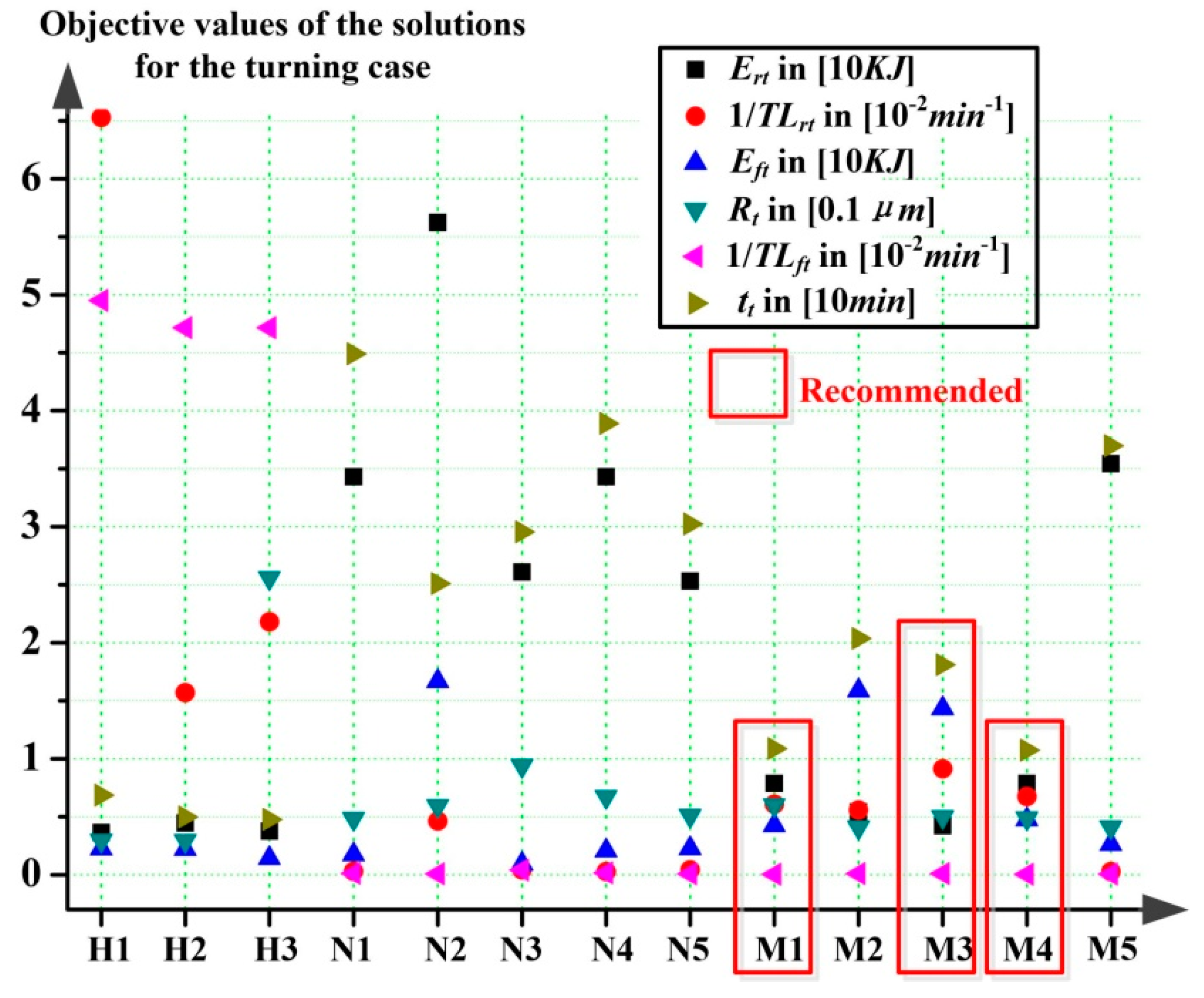
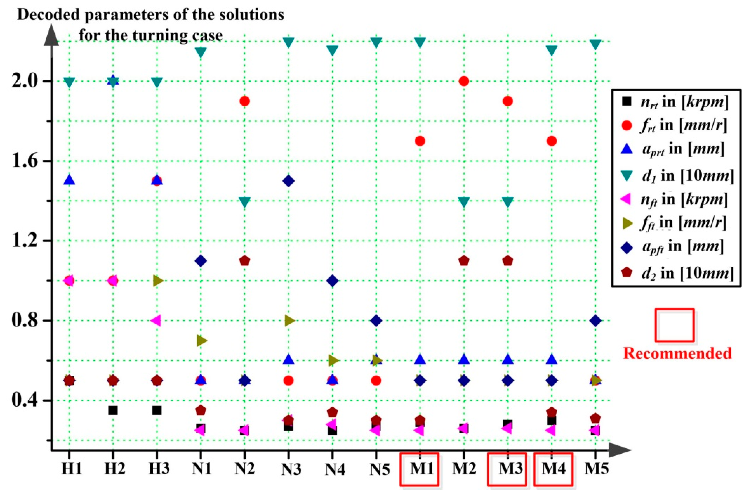
5.3.1. Analysis of the Turning Case

For the case of turning specifically, based on Figure 8 and Figure 9, the analysis results can be summarized in the following aspects:
First, the solutions of M1, M3, and M4 apparently outperformed other solutions in each aspect of optimization objective. They are the most recommended solutions used in future real production scenarios. By using this kind of solutions, with a little sacrifice of energy costs and efficiency, the other objectives can all be greatly improved compared to traditional methods from handbooks, especially for cutting tool life and surface roughness.
Second, based on the first analysis result and Figure 9, the decoded parameters and allowances of the most recommended solutions can be used as guidance for future process planning. Generally, the allowance of rough turning phase should be set around 21 to 22 mm, and the machining parameters should be set with a combination of low spindle rotation speed around 280 to 300 rpm, high feed rate around 1.7 to 1.9 mm/r and large cutting depth around 0.5 to 0.6 mm for rough turning. For finishing turning, it should be with allowance around 3 to 4 mm, spindle rotation speed around 250 to 260 rpm, low feed rate around 0.5 mm/r, and small cutting depth around 0.5 mm. The recommended ranges of machining allowances and related parameters of the turning case are listed in Table 20.
Third, there are not many improvements in the energy states when comparing the Pareto solutions with those obtained from handbooks. However, it is also obvious that they can significantly prolong the cutting tool life 200% to 500% longer estimably, and that is applicable both for the rough and finishing turning. This improvement will result in cutting down of resource use and production costs without harming the energy costs too much.

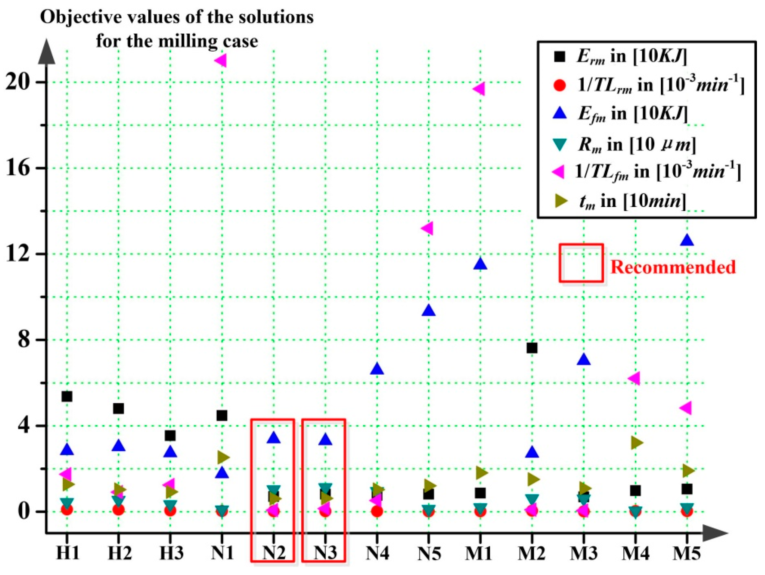
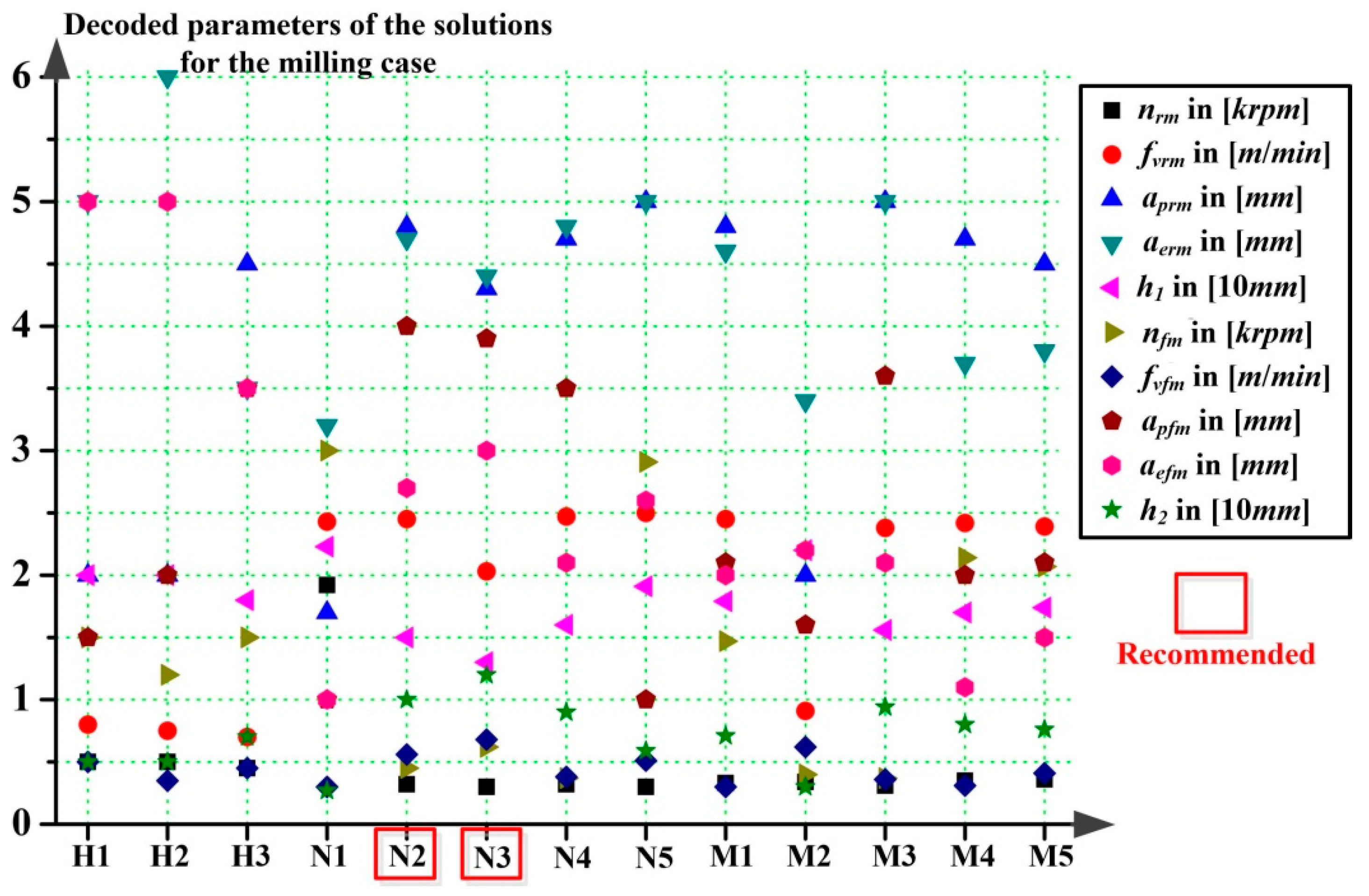
5.3.2. Analysis of the Milling Case

For the case of milling specifically, based on Figure 10 and Figure 11, the analysis results can be summarized in the following aspects:
First, the solutions of N2 and N3 apparently outperformed other solutions in each aspect, and they are the most recommended solutions. Specifically, the energy consumption of rough milling can be greatly reduced to around 20% of traditional methods from handbooks.
Second, based on Figure 11, the decoded parameters and allowances of N1 and N2 can be used as guidance for future process planning. Generally, the allowance of rough milling phase should be set around 13 to 15 mm, and the machining parameters should be set with a combination of low spindle rotation speed around 300 to 320 rpm, high feed speed around 2000 to 2500 mm/min, large cutting depth around 4.3 to 4.8 mm and small cutting width around 4.4 to 4.7 mm for rough milling. For finishing milling, it should be with allowance around 10 to 12 mm, spindle rotation speed around 450 to 620 rpm, feed speed around 560 to 680 mm/min, cutting depth around 4 mm and cutting width around 2.7 to 3 mm.
The recommended ranges of machining allowances and related parameters for the two cases are both listed in Table 20. From Table 20, workers can choose among those to meet various kinds of engineering demands accordingly.

5.3.3. Performance Evaluations of Algorithms and Related Discussion

The performance evaluation indicators I t and I n can be used to compare the intelligent algorithms. They can offer a reference for future algorithm determining strategies.
As Table 8 and Table 16 show, the solving speeds of NSGA-Ⅱ are faster than those of MOEA/D. However, MOEA/D generally outperformed NSGA-Ⅱ in finding effective Pareto solutions for the turning case, because of the diversity and fast solving speed as well. Namely, MOEA/D is more effective in providing solutions located in the area of multi-objective equilibrium for the turning case. Those solutions are more likely to be used in real engineering scenarios. And NSGA-Ⅱ is more suitable for the milling case, respectively, for the same reasons.

5.3.4. Discussions

Compared with previous research, the analysis results revealed facts of the following aspects:
(1)
Rather than parameter optimizations of a single machining phase like the works of [20,21], comprehensive optimization considering machining allowance distributions of different machining phases is more likely to be used in real production. The generated solutions provide not only energy-oriented machining parameters, but also various groups of parameters and allowances for better implementation. The priorities of each phase can all be met by doing so.
(2)
This research further enhances the recommendation of relative larger setting of machining allowance of rough machining, and small setting of finishing machining, like [4,26].
(3)
It is revealed that the high-speed cutting technique recommended by many previous studies, like [13,30], are not always suitable for application. Specifically, for multi-objective considerations like energy costs and tool protection, relative low cutting speeds of the finishing phases are recommended in this research.
(4)
Contrary to our previous finding of [27], NSGA-Ⅱ outperformed MOEA/D in the milling case once machining allowance distribution is involved. Namely, the selection of optimization strategies should be well-adjusted, considering the characteristics and uniqueness of the specific problem.

6. Conclusions and Future Work

The major contributions of the research are listed as follows:
(1)
Improved modeling of machining allowance distribution is proposed, integrated with parameter optimization. Energy-saving demands of different machining phases can be comprehensively met. With the machining allowance distribution well-addressed, the proposed method is relatively practical compared to traditional methods, consistent with the actual situation.
(2)
The most recommended optimization solutions are picked out, and they can be used in real production directly. Workers can choose among those non-determined solutions for their optimization priority, without harming any of the economic objectives too much. With a little sacrifice of energy costs and efficiency, cutting tool life and surface roughness can all be greatly improved for turning, and energy consumption of rough milling can be greatly reduced to around 20% of traditional methods.
(3)
The most suitable scope of machining allowances and parameters is precisely recommended. It can be concluded that during rough machining, the machining should be set with the combination of large allowance, high cutting speed, high feed rate and large cutting depth. During finish machining, it should be the combination of small allowance, low cutting speed, low feed speed, and small cutting depth.
(4)
The performance of different strategies, including and MOEA/D was studied. The selection of algorithms can be adjusted as needed considering the performance analysis. Generally, MOEA/D is more likely to be used for turning and NSGA-Ⅱ is more likely to be used for milling for real applications.
The limits of this research are listed as follows:
(1)
So far, only cylindrical turning and step milling have been studied. Other machining scenarios and demands, like drilling, grinding, and complex surface machining, are necessary to further validate the proposed method should be considered.
(2)
How do the limitations and constraints used affect the results has not been not discussed. Factors like high-speed cutting technique, machine tolerance changes, cutting tool conditions, and change of cooling paths will affect the results.
(3)
The possibility of uncertainty will affect the results, like the changes of machine types, layouts, cutting tools, materials, and optimization priorities.
As the next step, we will investigate other machining processes and situations, like drilling and grinding. And the definition of limitations and constraints should be well-adjusted according to the scenario. For example, the high-speed cutting technique may have a great influence on the results, which deserve further investigation. Rather than intelligent algorithms we used, the performance of other optimization techniques will be studied. We will study how to incorporate the proposed method to uncertainties of changes, such as choice of machines, materials and cutting tools, etc.

Author Contributions

Conceptualization, K.H.; methodology, K.H. and H.H.; software, K.H. and H.H.; validation, K.H.; formal analysis, K.H. and J.W.; investigation, K.H.; resources, R.T.; data curation, K.H. and J.W.; writing—original draft preparation, K.H.; writing—review and editing, H.H. and R.T.; visualization, K.H.; supervision, H.H. and R.T.; project administration, H.H. and R.T.; funding acquisition, R.T. and K.H. All authors have read and agreed to the published version of the manuscript.

Funding

This research was funded by National Natural Science Foundation of China, grant number U1501248 and China Postdoctoral Science Foundation, grant number 47662 (the 66th batch of the military system).

Acknowledgments

The authors would like to convey their sincere thanks to Jilie Zhou and Qiang Wang from the metalworking center of Zhejiang University for their valuable contributions during the experiments. We also thank Jingxiang Lv, Jia Shun, Jun Zheng and all the anonymous reviewers for their helpful suggestions on the quality improvement of our paper.

Conflicts of Interest

The authors declare no conflicts of interest.

Nomenclature

a e m , a e r m , a e f m
a e m m a x
Cutting width of milling, those of rough milling and finishing milling, and their maximum value according to the scenario [mm]
a p t , a p r t , a p f t
a p m , a p r m , a p f m
Cutting depth of turning, and those of rough turning, finishing turning, general milling, rough milling and finishing milling [mm]
a p t m a x , a p m m a x Maximum values of cutting depths according to the turning or milling scenario [mm]
C c t ,   C v c t , C f c t , C a p c t
C c m ,   C n c m , C f c m ,
C a p c m , C a e c m
Coefficients of the polyphyletic function for material cutting power of turning and those of milling
C f 1 , C f 2 Coefficients of the quadratic function for feed power calculation
C R a m , C R a v m ,   C R a f m C R a a p m , C R a a e m Coefficients of the function for roughness of workpieces after milling process
C r A 1 ,   C r A 2
C r B 1 ,   C r B 2
C r C 1 ,   C r C 2
Coefficients of the three linear functions for spindle rotation power calculation
C T L t , C T L t v
C T L t f , C T L t a p
Coefficients of the function for cutting tool life after turning
C T L m , C T L m v
C T L m f , C T L m a p
C T L m a e
Coefficients of the function for cutting tool life after milling
D T Diameter of the cutting tool of milling [mm]
D Value range of variables of a sub-objective function
d , d 1 , d 2 Radial distance of the workpiece to be tooled of turning, and those for rough tuning and finishing turning [mm]
E r t , E r t
E f t , E f t
E r m , E r m
E f m , E f m
Energy consumption of rough turning, its normalized expression, and those for finishing turning, rough milling and finishing milling [J]
E o Energy consumption objective during a machining process [J]
f t , f r t , f f t
f m , f r m , f f m
Feed rates of general turning, and those of rough turning, finishing turning, general milling, rough milling, and finishing milling [mm/r]
f t m a x , f m m a x Maximum values of feed rates according to the turning or milling scenario [mm/r]
f v t , f v r t , f v f t
f v m , f v r m , f v f m
Feed speeds of general turning, and those of rough turning, finishing turning, general milling, rough milling and finishing milling [mm/min]
f v t m a x , f v m m a x Maximum values of feed speeds according to the turning or milling scenario [mm/min]
f i ( X ) , f i ( X ) One of the sub-objective functions and its normalized expression
h , h 1 , h 2 Total height of the workpiece to be tooled of milling, and those for rough milling and finishing milling [mm]
I n Number of effective Pareto solutions an algorithm can obtain finally
I t Average operating time for a certain number of repeats of the solving operation [s]
L s t , L s m Length of feed path for one single cutting of turning and milling [mm]
l t , l m Total axial lengths of the workpiece to be tooled of turning and milling [mm]
M , G , R c
R m , N , m
Initial population, gap between two generations, crossover rate, mutation rate, maximum evolution generations and length of the genes of basic genetic algorithm
M R R , M R R t , M R R m Material removal rate, and those of turning and milling [mm3/min]
N t Feed times needed to cut the whole volume to be tooled of a turning process
n Spindle rotation speed of machining processes [rpm]
n I Number of the operation repeats to evaluate the algorithm
n t , n r t , n f t
n m , n r m , n f m
Spindle rotation speed of general turning, those of rough turning and finishing turning, and those of general milling, rough milling and finishing milling [rpm]
n t m a x , n m m a x Maximum values of spindle rotation speeds according to the turning or milling scenario [rpm]
n M B A ,   n M l Turning points of the three linear functions for spindle rotation power calculation
P b , P s , P r , P f , P c   Power of basic machine motion, spraying cooling fluid, spindle rotation, feed movement, material cutting [W]
P c t ,   P c m Material cutting power of turning and milling [W]
p h ball screw lead [mm]
R Radius of the original cylindrical material to be tooled [mm]
R a t , R a t
R a m , R a m
Surface roughness of the workpiece after turning, its normalized expression, and those for milling [μm]
r ε , κ r , κ r Corner radius, main cutting edge angle and secondary cutting edge angle of the cutting tool
S n e i , S t o u r Sizes of neighbor and tournament of MOEA/D algorithm
T L O A constant for a given feed drive system
T L r t , T L r t
T L f t , T L f t
T L r m , T L r m
T L f m , T L f m
Tool life of rough turning, its normalized expression, and those for finishing turning, rough milling and finishing milling [min]
t c , t c t , t c m Material cutting time of machining processes, and those of turning and milling [min]
t c r t , t c f t
t c r m , t c f m
Material cutting time of rough turning and finishing turning, and those of rough milling and finishing milling [min]
t f , t f t , t f m Feeding time of machining processes, and those of turning and milling [min]
t f r t , t f f t
t f r m , t f f m
Feeding time of rough turning and finishing turning, and those of rough milling and finishing milling [min]
t i Lasting time of a single optimization operation [s]
t o Time objective during a machining process [min]
V , V t , V m Total workpiece volumes to be tooled, and those in a turning process and milling process [mm3]
v t , v r t , v f t
v m , v r m , v f m
Cutting speeds of general turning, and those of rough turning, finishing turning, rough milling and finishing milling [m/min]
v t m a x , v m m a x Maximum values of cutting speeds according to the turning or milling scenario [m/min]

References

  1. Lv, J.; Gu, F.; Zhang, W.; Guo, J. Life cycle assessment and life cycle costing of sanitary ware manufacturing: A case study in China. J. Clean. Prod. 2019, 238, 117938. [Google Scholar] [CrossRef]
  2. Yang, F.; Liu, Y.; Liu, G. A process simulation based benchmarking approach for evaluating energy consumption of a chemical process system. J. Clean. Prod. 2016, 112, 2730–2743. [Google Scholar] [CrossRef]
  3. Kassai, M.; Poleczky, L.; Alhyari, L.; Kajtar, L.; Nyers, J. Investigation of the Energy Recovery Potentials in Ventilation Systems in Different Climates. Facta Univ. Ser. Mech. Eng. 2018, 16, 203–217. [Google Scholar] [CrossRef] [Green Version]
  4. Wu, X.; Dai, W. Research on Machining Allowance Distribution Optimization based on Processing Defect Risk. Procedia CIRP 2016, 56, 508–511. [Google Scholar] [CrossRef] [Green Version]
  5. International Energy Agency. World Energy Outlook 2016; International Energy Agency: Paris, France, 2016. [Google Scholar]
  6. Dunham, S. Inventory of U.S. Greenhouse Gas Emissions and Sinks: 1990–2013; US EPA: Washington, DC, USA, 2015.
  7. Zhang, Y.; Zhang, D.; Wu, B. An approach for machining allowance optimization of complex parts with integrated structure. J. Comput. Des. Eng. 2015, 2, 248–252. [Google Scholar] [CrossRef] [Green Version]
  8. Kassai, M.; Ge, G.; Simonson, C.J. Dehumidification performance investigation of run-around membrane energy exchanger system. Therm. Sci. 2016, 20, 1927–1938. [Google Scholar] [CrossRef]
  9. EIA. U.S. Energy-Related Carbon Dioxide Emissions, 2014. 2014. Available online: https://www.eia.gov/environment/emissions/carbon/archive/2014/pdf/2014_co2analysis.pdf (accessed on 15 January 2020).
  10. Zhang, Z.; Wu, L.; Peng, T.; Jia, S. An Improved Scheduling Approach for Minimizing Total Energy Consumption and Makespan in a Flexible Job Shop Environment. Sustainability 2019, 11, 179. [Google Scholar] [CrossRef] [Green Version]
  11. Kant, G.; Sangwan, K.S. Prediction and optimization of machining parameters for minimizing power consumption and surface roughness in machining. J. Clean. Prod. 2014, 83, 151–164. [Google Scholar] [CrossRef]
  12. Lv, J.; Tang, R.; Tang, W.; Jia, S.; Ying, L.; Cao, Y. An investigation into methods for predicting material removal energy consumption in turning. J. Clean. Prod. 2018, 193, 128–139. [Google Scholar] [CrossRef] [Green Version]
  13. Jia, S.; Yuan, Q.; Cai, W.; Lv, J.; Hu, L. Establishing prediction models for feeding power and material drilling power to support sustainable machining. Int. J. Adv. Manuf. Technol. 2019, 100, 2243–2253. [Google Scholar] [CrossRef]
  14. Franco, A.; Rashed, C.A.A.; Romoli, L. Analysis of energy consumption in micro-drilling processes. J. Clean. Prod. 2016, 137, 1260–1269. [Google Scholar] [CrossRef]
  15. Sealy, M.P. Energy consumption and modeling in precision hard milling. J. Clean. Prod. 2015, 135, 1591–1601. [Google Scholar] [CrossRef]
  16. Aramcharoen, A.; Mativenga, P.T. Critical factors in energy demand modelling for CNC milling and impact of toolpath strategy. J. Clean. Prod. 2014, 78, 63–74. [Google Scholar] [CrossRef]
  17. Pusavec, F.; Kramar, D.; Krajnik, P.; Kopac, J. Transitioning to sustainable production-part II: Evaluation of sustainable machining technologies. J. Clean. Prod. 2010, 18, 1211–1221. [Google Scholar] [CrossRef]
  18. Li, C.; Chen, X.; Ying, T.; Li, L. Selection of optimum parameters in multi-pass face milling for maximum energy efficiency and minimum production cost. J. Clean. Prod. 2017, 140, 1805–1818. [Google Scholar] [CrossRef]
  19. Albertelli, P.; Keshari, A.; Matta, A. Energy oriented multi cutting parameter optimization in face milling. J. Clean. Prod. 2016, 137, 1602–1618. [Google Scholar] [CrossRef]
  20. Wang, Q.; Liu, F.; Wang, X. Multi-objective optimization of machining parameters considering energy consumption. Int. J. Adv. Manuf. Technol. 2014, 71, 1133–1142. [Google Scholar] [CrossRef]
  21. Yan, J.; Li, L. Multi-objective optimization of milling parameters-the trade-offs between energy, production rate and cutting quality. J. Clean. Prod. 2013, 52, 462–471. [Google Scholar] [CrossRef]
  22. Camposeco-Negrete, C. Prediction and optimization of machining time and surface roughness of AISI O1 tool steel in wire-cut EDM using robust design and desirability approach. Int. J. Adv. Manuf. Technol. 2019, 103, 2411–2422. [Google Scholar] [CrossRef]
  23. Wei, Z.C.; Guo, M.L.; Wang, M.J.; Li, S.Q.; Liu, S.X. Prediction of cutting force of ball-end mill for pencil-cut machining. Int. J. Adv. Manuf. Technol. 2018, 100, 577–588. [Google Scholar] [CrossRef]
  24. Hanafi, I.; Khamlichi, A.; Cabrera, F.M.; Almansa, E.; Jabbouri, A. Optimization of cutting conditions for sustainable machining of PEEK-CF30 using TiN tools. J. Clean. Prod. 2012, 33, 1–9. [Google Scholar] [CrossRef]
  25. Zhang, Z.; Ming, L.; Zhang, D.; Wu, B. A force-measuring-based approach for feed rate optimization considering the stochasticity of machining allowance. Int. J. Adv. Manuf. Technol. 2018, 97, 2545–2556. [Google Scholar] [CrossRef]
  26. Jiang, S.; Li, Y.; Liu, C. A non-uniform allowance allocation method based on interim state stiffness of machining features for NC programming of structural parts. Vis. Comput. Ind. Biomed. Art 2018, 1, 4. [Google Scholar] [CrossRef]
  27. He, K.; Tang, R.; Jin, M. Pareto fronts of machining parameters for trade-off among energy consumption, cutting force and processing time. Int. J. Prod. Econ. 2017, 185, 113–127. [Google Scholar] [CrossRef]
  28. He, K.; Tang, R.; Zhang, Z.; Sun, W. Energy Consumption Prediction System of Mechanical Processes Based on Empirical Models and Computer-Aided Manufacturing. J. Comput. Inf. Sci. Eng. 2016, 16, 041008. [Google Scholar] [CrossRef]
  29. Lv, J.; Tang, R.; Jia, S. Therblig-based energy supply modeling of computer numerical control machine tools. J. Clean. Prod. 2014, 65, 168–177. [Google Scholar] [CrossRef]
  30. Lv, J.; Tang, R.; Jia, S.; Ying, L. Experimental study on energy consumption of computer numerical control machine tools. J. Clean. Prod. 2016, 112, 3864–3874. [Google Scholar] [CrossRef] [Green Version]
  31. Lv, J.; Tang, R.; Tang, W.; Ying, L.; Zhang, Y.; Jia, S. An investigation into reducing the spindle acceleration energy consumption of machine tools. J. Clean. Prod. 2016, 143, 794–803. [Google Scholar] [CrossRef] [Green Version]
  32. Jia, S.; Yuan, Q.; Cai, W.; Li, M.; Li, Z. Energy modeling method of machine-operator system for sustainable machining. Energy Convers. Manag. 2018, 172, 265–276. [Google Scholar] [CrossRef]
  33. Jia, S.; Yuan, Q.; Lv, J.; Liu, Y.; Ren, D.; Zhang, Z. Therblig-embedded value stream mapping method for lean energy machining. Energy 2017, 138, 1081–1098. [Google Scholar] [CrossRef] [Green Version]
  34. Nee, A.Y.C. Handbook of Manufacturing Engineering and Technology; Springer Verlag: London, UK, 2014; pp. 569–592. [Google Scholar]
  35. Grote, K.H.; Antonsson, E.K. Springer Handbook of Mechanical Engineering; Springer Verlag: New York, NY, USA, 2009; pp. 1–33. [Google Scholar]
  36. Sun, Y.W.; Xu, J.T.; Guo, D.M.; Jia, Z.Y. A unified localization approach for machining allowance optimization of complex curved surfaces. Precis. Eng. 2009, 33, 516–523. [Google Scholar] [CrossRef]
  37. Armarego, E.J.A.; Brown, R.H. The machining of metals. Wear 1969, 14, 305. [Google Scholar]
  38. Wu, D.; Zhou, Y. Modeling and Experimental Study on Tool Wear Life in High-speed Milling. Manuf. Technol. Mach. Tool 2008, 11, 90–93. [Google Scholar]
  39. Xiao, Y.; Zhang, H.; Jiang, Z. An approach for blank dimension design considering energy consumption. Int. J. Adv. Manuf. Technol. 2015, 10, 1229–1238. [Google Scholar] [CrossRef]
  40. Deb, K.; Pratap, A.; Agarwal, S.; Meyarivan, T. A fast and elitist multiobjective genetic algorithm: NSGA-II. IEEE Trans. Evol. Comput. 2002, 6, 182–197. [Google Scholar] [CrossRef] [Green Version]
  41. Zhang, Q.; Li, H. MOEA/D: A Multiobjective Evolutionary Algorithm Based on Decomposition. IEEE Trans. Evol. Comput. 2007, 11, 712–731. [Google Scholar] [CrossRef]
  42. Rowe, G.W. Principles of machining by cutting, abrasion and erosion. Wear 1978, 49, 393–394. [Google Scholar] [CrossRef]
Figure 1. The overall flow of this research.
Sustainability 12 00638 g001
Figure 2. Machining allowance distribution of a cylindrical turning.
Sustainability 12 00638 g002
Figure 3. Machining allowance distribution of a step milling.
Sustainability 12 00638 g003
Figure 4. Power profile of a typical milling process [28].
Sustainability 12 00638 g004
Figure 5. Diagram of experimental set-up [32].
Sustainability 12 00638 g005
Figure 6. A case of cylindrical turning process.
Sustainability 12 00638 g006
Figure 7. A case of step milling process.
Sustainability 12 00638 g007
Figure 8. Objective values of the solutions for the case of turning.
Sustainability 12 00638 g008
Figure 9. Decoded parameters of the solutions for the case of turning.
Sustainability 12 00638 g009
Figure 10. Objective values of the solutions for the case of milling.
Sustainability 12 00638 g010
Figure 11. Decoded parameters of the solutions for the case of milling.
Sustainability 12 00638 g011
Table 1. Cutting parameters, optimization objectives and machining allowances.
Machining TypeTurning ProcessMilling Process
Machining phasesRough turningFinish turningRough millingFinish milling
Machining
parameters
Cutting speed vrt
Spindle speed nrt
Feed speed fvrt
Feed rate frt
Cutting depth aprt
Cutting speed vft
Spindle speed nft
Feed speed fvft
Feed rate fft
Cutting depth apft
Cutting speed vrm
Spindle speed nrt
Feed speed fvrm
Feed rate frm
Cutting depth aprm
Cutting width aerm
Cutting speed vfm
Spindle speed nft
Feed speed fvfm
Feed rate ffm
Cutting depth apfm
Cutting width aefm
Optimization objectivesEnergy consumption Ert
Cutting time trt
Cutting tool life TLrt
Energy consumption Eft
Cutting time tft
Surface roughness RatCutting tool life TLft
Energy consumption Erm
Cutting time trm
Cutting tool life TLrm
Energy Efm
Cutting time tfm
Surface roughness RamCutting tool life TLfm
Machining allowanceRadial distance for rough turning d1Radial distance for finish turning d2Height of the workpiece for rough milling h1Height of the workpiece for finish milling h2
Table 2. Operating parameters of GA.
Operating ParametersRemarksValues
M Size of the initial population500
G Gap between parents and children0.9
  R c Crossover rate0.7
  R m Mutation rate0.7/Lind
N The maximum evolution generations300
Table 3. Geometrical parameters of VNMG160408-YBC351 cutting tool.
Clearance   angle   α o 7 °
Main cutting edge angle κ r 93 °
Secondary cutting edge angle κ r 52 °
Corner radius r ε 0.8 mm
Table 4. Taguchi experiment levels of turning parameters.
Turning ParametersLevel 1Level 2Level 3Level 4
Cutting speed v t   [ m / min ] 50100150200
Feed rate f t   [ mm / r ] 0.050.10.150.2
Cutting depth a p t   [ mm ] 0.511.52
Table 5. Parameter design matrix of turning experiments.
Experiment OrderTurning Parameters
Cutting Speed
v t   [ m / m i n ]
Feed Rate
f t   [ m m / r ]
Cutting Depth
a p t   [ m m ]
1500.050.5
2500.11
3500.151.5
4500.22
51000.051
61000.10.5
71000.152
81000.21.5
91500.051.5
101500.12
111500.150.5
121500.21
132000.052
142000.11.5
152000.151
162000.20.5
Table 6. Constrains of machining parameters for this turning process.
Machining ParametersConstrains
Cutting speed v t 0   m / min v t 200   m / min
Rotation speed n t 100   r / min n t 1500   r / min
Feed rate f t 0.1   mm / r f t 2   mm / r
Cutting depth a p t 0.1   mm a pt 5   mm
Table 7. Calculation results of value ranges of sub-object functions.
Objectives
(st: Constrains)
E r t 1 / T L r t E f t R a t 1 / T L f t t t
Minimum values0 3.765 × 10 8 0 1.563 × 10 3 3.765 × 10 8 0.205
Maximum values 2.322 × 10 7 428.456 2.322 × 10 7 1.028101.6753210.167
Table 8. Performance evaluation indexes for the objective turning process.
Performance Evaluation Indexes I t [ s ] I n
NSGA-II34.5306
MOEA/D17.5355
Table 9. Simulation experiment data of objective turning process.
Solution Type:Data of Validation Experiments (Average of Five Repeats):
Ert [J]TLrt [min]Eft [J]Rat [μm]TLft [min]tt [min]
Solutions from handbooksNo. 1 3.653 × 10 4 15.324 2.243 × 10 4 2.954 × 10 2 20.2356.864
No. 2 4.456 × 10 4 63.678 2.223 × 10 4 2.926 × 10 2 21.2344.987
No. 3 3.764 × 10 4 45.865 1.445 × 10 4 2.558 × 10 1 21.2384.765
Pareto solutions from NSGA-IINo. 1 3.431 × 10 5 3.456 × 10 3 1.746 × 10 4 4.827 × 10 2 7.856 × 10 3 44.908
No. 2 5.623 × 10 5 215.353 1.669 × 10 5 5.927 × 10 2 1.368 × 10 4 25.098
No. 3 2.612 × 10 5 2.345 × 10 3 9.325 × 10 3 9.398 × 10 2 2.454 × 10 3 29.564
No. 4 3.432 × 10 5 3.569 × 10 3 2.076 × 10 4 6.725 × 10 2 6.621 × 10 3 38.908
No. 5 2.532 × 10 5 2.324 × 10 3 2.278 × 10 4 5.098 × 10 2 1.382 × 10 4 30.235
Pareto solutions from MOEA/DNo. 1 7.876 × 10 4 164.098 4.259 × 10 4 5.987 × 10 2 2.766 × 10 4 10.874
No. 2 5.432 × 10 4 179.098 1.587 × 10 5 4.092 × 10 2 1.047 × 10 4 20.375
No. 3 4.234 × 10 4 109.543 1.434 × 10 5 4.987 × 10 2 9.647 × 10 3 18.098
No. 4 7.875 × 10 4 147.987 4.778 × 10 4 4.876 × 10 2 2.663 × 10 4 10.75
No. 5 3.543 × 10 5 3.523 × 10 3 2.648 × 10 4 4.098 × 10 2 1.787 × 10 4 36.985
Table 10. Decoded solutions of objective turning process.
Solution TypeRelevant Decoded Parameters
nrt
[rpm]
frt
[mm/r]
aprt
[mm]
d1
[mm]
nft
[rpm]
fft
[mm/r]
apft
[mm]
d2
[mm]
Solutions from handbooksNo. 15001.01.520.010000.50.55.0
No. 23501.02.020.010000.50.55.0
No. 33501.51.520.08001.00.55.0
Pareto solutions from NSGA-IINo. 12600.50.521.52500.71.13.5
No. 22501.90.514.02500.50.511.0
No. 32700.50.622.03000.81.53.0
No. 42500.50.521.62800.61.03.4
No. 52700.50.622.02500.60.83.0
Pareto solutions from MOEA/DNo. 12901.70.622.02500.50.53.0
No. 22602.00.614.02600.50.511.0
No. 32801.90.614.02600.50.511.0
No. 43001.70.621.62500.50.53.4
No. 52500.50.521.92500.50.83.1
Table 11. Deviations of the objective turning models.
Solution TypeDeviation Percentages of the Models:
ErtEftRattt
Solutions from handbooksNo. 13.533%5.421%2.544%5.422%
No. 24.652%5.644%1.235%5.642%
No. 32.451%4.324%2.654%4.765%
Pareto solutions from NSGA-IINo. 14.311%4.655%2.654%5.235%
No. 21.235%5.654%1.654%5.423%
No. 34.321%3.434%3.543%3.644%
No. 43.543%5.655%2.533%4.643%
No. 53.342%3.654%1.644%4.542%
Pareto solutions from MOEA/DNo. 14.325%5.422%1.952%5.321%
No. 21.652%4.345%1.744%5.322%
No. 34.311%3.654%2.652%4.564%
No. 45.323%5.312%2.654%4.653%
No. 54.345%2.534%3.443%3.564%
Table 12. Taguchi experiment levels of milling parameters.
Milling ParametersLevel 1Level 2Level 3Level 4
Rotation speed n m   [ rpm ] 10050015003000
Feed speed f v m   [ mm / r ] 10050015003000
Cutting depth a p m   [ mm ] 0.1135
Cutting width a e m   [ mm ] 0.1135
Table 13. Parameter design matrix of milling experiments.
Experiment OrderMilling Parameters
Rotation   Speed   n m   [ r p m ] Feed   Speed   f v m   [ m m / r ] Cutting   Depth   a p m   [ m m ] Cutting   Width   a e m   [ m m ]
11001000.10.1
210050011
3100150033
4100300055
550010035
650050053
750015000.11
8500300010.1
9150010051
10150050030.1
111500150015
12150030000.13
13300010013
1430005000.15
153000150050.1
163000300031
Table 14. Constrains of machining parameters for this milling process.
Machining ParametersConstrains
Rotation speed n m 100   r / min n m 6000   rpm
Cutting speed v m 0   m / min v m 200   m / min
Feed speed f m 100   mm / r f m 8000   mm / min
Cutting depth a p m 0.1   mm a p m 5   mm
Cutting width a e m 0.1   mm a e m 5   mm
Table 15. Calculation results of value ranges of sub-object functions.
Objectives
(St: Constrains)
E r m 1 / T L r m E f m R a m 1 / T L f m t m
Minimum values0 6.466 × 10 15 0 5.750 × 10 3 6.466 × 10 15 0.406
Maximum values 5.306 × 10 8 6.360 × 10 9 5.306 × 10 8 293.712 6.360 × 10 9 8.125 × 10 4
Table 16. Performance evaluation indexes for the objective step milling process.
Performance Evaluation Indexes I t I n
NSGA-II46.43354
MOEA/D23.54287
Table 17. Validation experiment data of objective step milling process.
Solution TypeData of Validation Experiments (Average of Five Repeats):
Erm [J]TLrm [min]Efm [J]Ram [μm]TLfm [min]tm [min]
Solutions from handbooksNo. 1 5.364 × 10 4 9.783 × 10 4 2.835 × 10 4 4.375 5.732 × 10 3 12.734
No. 2 4.803 × 10 4 1.032 × 10 5 3.016 × 10 4 5.395 1.094 × 10 4 10.285
No. 3 3.545 × 10 4 1.721 × 10 5 2.733 × 10 4 3.294 8.041 × 10 3 9.273
Pareto solutions from NSGA-ⅡNo. 1 4.476 × 10 4 3.227 × 10 5 1.756 × 10 4 0.864 4.762 × 10 2 25.293
No. 2 7.024 × 10 3 5.174 × 10 5 3.388 × 10 4 10.284 1.437 × 10 5 6.092
No. 3 8.167 × 10 3 5.466 × 10 5 3.305 × 10 4 11.245 6.928 × 10 4 6.235
No. 4 7.554 × 10 3 5.223 × 10 5 6.593 × 10 4 9.457 1.915 × 10 4 10.283
No. 5 8.125 × 10 3 6.327 × 10 5 9.318 × 10 4 1.092 7.585 × 10 2 12.083
Pareto solutions from MOEA/DNo. 1 8.676 × 10 3 4.826 × 10 5 1.148 × 10 5 1.863 5.083 × 10 2 18.092
No. 2 7.625 × 10 4 2.138 × 10 5 2.713 × 10 4 6.098 1.082 × 10 5 15.098
No. 3 6.956 × 10 3 5.913 × 10 5 7.033 × 10 4 5.987 1.867 × 10 5 10.875
No. 4 9.825 × 10 3 3.772 × 10 5 2.494 × 10 5 0.345 1.612 × 10 3 32.098
No. 5 1.056 × 10 4 3.543 × 10 5 1.259 × 10 5 1.972 2.072 × 10 3 19.092
Table 18. Decoded solutions of objective step milling process.
Solution TypeRelevant Decoded Parameters
nrm
[rpm]
fvrm
[mm/min]
aprm
[mm]
aerm
[mm]
h1
[mm]
nfm
[rpm]
fvfm
[mm/min]
apfm
[mm]
aefm
[mm]
h2
[mm]
Solutions from handbooksNo. 15008002.05.020.015005001.55.05.0
No. 25007502.06.020.0120035025.05.0
No. 34507004.53.518.015004503.53.57.0
Pareto solutions from NSGA-IINo. 1192024301.73.222.330003001.01.02.7
No. 232024504.84.715.04505604.02.710.0
No. 330020304.34.413.06206803.93.012.0
No. 432024704.74.816.03703803.52.19.0
No. 530025005.05.019.129105101.02.65.9
Pareto solutions from MOEA/DNo. 133024504.84.617.914703002.12.07.1
No. 23409102.03.422.04006201.62.23.0
No. 331023805.05.015.63703603.62.19.4
No. 435024204.73.717.021403102.01.18.0
No. 536023904.53.817.420704102.11.57.6
Table 19. Deviations of the objective milling models.
Solution TypeDeviation Percentages of the Models:
ErmEfmRamtm
Solutions from handbooksNo. 12.633%4.765%1.353%4.986%
No. 23.563%4.654%1.653%4.844%
No. 34.321%4.654%1.653%4.876%
Pareto solutions from NSGA-IINo. 13.533%4.953%3.234%4.876%
No. 22.542%4.568%2.422%4.327%
No. 33.653%4.567%3.675%3.874%
No. 44.312%4.965%1.563%3.876%
No. 52.564%4.345%1.784%4.875%
Pareto solutions from MOEA/DNo. 14.642%4.653%1.895%4.873%
No. 24.565%4.865%1.752%3.543%
No. 34.654%4.953%2.236%3.765%
No. 44.654%4.843%2.963%4.886%
No. 54.964%4.754%3.326%3.986%
Table 20. Recommended scope of machining parameters for case No. 1 and No. 2.
Case InformationCylindrical Turning
(Case No. 1)
Face Milling (Case No. 2)
Mechanical scenarioMachineCK6153i-AHXHK-714F
CutterVNMG160408-YBC351W400-FS
Blank workpieceCACE45CACE45
Cutting typeWet cuttingWet cutting
Total allowanced = 25H = 25
Machining allowances and parametersRough machining phaseSpindle speed [rpm]280 < nrt < 300300 < nrm < 320
Feed speed [mm/min] or feed rate [mm/r]1.7 < frt < 1.92000 < fvrm < 2500
Cutting depth [mm]0.5 < aprt < 0.64.3 < aprm < 4.8
Cutting width [mm]/4.4 < aerm < 4.7
Allowance [mm]21.0 < d1 < 22.016.0 < h1 < 22.0
Finishing machining phaseSpindle speed [rpm]250 < nft < 260450 < nfm < 620
Feed speed [mm/min] or feed rate [mm/r]fft ≈ 0.5560 < fvfm < 680
Cutting depth [mm]apft ≈ 0.5apfm ≈ 4.0
Cutting width [mm]/2.7 < aefm < 3.0
Allowance [mm]3.0 < d2 < 4.010.0 < h2 < 12.0

