Spatiotemporal Trends and Attribution of Drought across China from 1901–2100

Abstract

Investigating long-term drought trends is of great importance in coping with the adverse effects of global warming. However, little attention has been focused on studying the detailed spatial variability and attribution of drought variation in China. In this study, we first generated a 1 km resolution monthly climate dataset for the period 1901–2100 across China using the delta spatial downscaling method to assess the variability of the Standardized Precipitation Evaporation Index (SPEI). We then developed a simple approach to quantifying the contributions of water supply (precipitation) and demand (potential evapotranspiration, PET) on SPEI variability, according to the meaning of the differentiating SPEI equation. The results indicated that the delta framework could accurately downscale and correct low-spatial-resolution monthly temperatures and precipitation from the Climatic Research Unit and general circulation models (GCMs). Of the 27 GCMs analyzed, the BNU-ESM, CESM1-CAM5, and GFDL-ESM2M were found to be the most accurate in modeling future temperatures and precipitation. We also found that, compared with the past (1901–2017), the climate in the future (2018–2100) will tend toward significant droughts, although both periods showed a high spatial heterogeneity across China. Moreover, the proportion of areas with significantly decreasing SPEI trends was far greater than the proportion of those with increasing trends in most cases, especially for northwestern and northern China. Finally, the proposed approach to quantifying precipitation and PET contributions performed well according to logical evaluations. The percentage contributions of precipitation and PET on SPEI variability varied with study periods, representative concentration pathway scenarios, trend directions, and geographic spaces. In the past, PET contributions for significant downward trends and precipitation contributions for significantly upward trends accounted for 95% and 72%, while their future contributions were 57 ± 22%–149 ± 20% and 95 ± 27%–190 ± 58%, respectively. Overall, our results provide detailed insights for planning flexible adaptation and mitigation strategies to cope with the adverse effects of climate drought across China.

1. Introduction

Several recent studies have suggested that ongoing warming is accelerating evaporation [1] and creating more spatiotemporal heterogeneity in precipitation [2] than in the past. This process will result in various complications due to drought for plant growth, crop yield, and other human activities [1,3,4,5]. China is home to multiple climate zones that host important agricultural regions and other societally important activities [5] that are likely to be affected by increased drought. Therefore, it is essential to investigate the detailed spatiotemporal change in the trend and attribution of drought across China, so as to develop sustainable plans for coping with the adverse effects of global climate change.

Several indexes have been employed to investigate long-term drought, including the standardized precipitation index [6], the Palmer drought severity index [7], and the standardized precipitation evapotranspiration index (SPEI) [8]. Unlike the standardized precipitation index, the SPEI considers changes in both the precipitation and the potential evapotranspiration induced by temperature [9,10]. The SPEI also allows for multiple temporal scales, unlike the Palmer drought severity index. The time scales of SPEI correspond to flexible climate drought research at different time scales, such as SPEI at 1, 3, and 12 months for the monthly, seasonal, and annual studies [8]. Moreover, because of the introduction of precipitation and evapotranspiration, SPEI can represent the surface moisture balance, and allows us to separate and quantify the influence of moisture supply and demand on drought variability [1,11]. This separation is useful for unraveling the future contributions of precipitation versus those of potential evapotranspiration (PET) to future trends in SPEI, and then enhancing our understanding of how global warming affects climatic drought.

At present, SPEI is often estimated globally through station observations [12,13,14] or climate datasets released by climate research organizations [1,9,10,15,16,17,18,19,20]. However, the detailed spatial patterns of SPEI cannot be obtained from these sources because of the current low densities of weather stations and the low spatial resolutions (e.g., >50 km per grid cell) of climate datasets [21,22]. This spatial uncertainty prevents the development of suitable adaptation and mitigation strategies at fine spatial scales [23,24,25]. Therefore, there is an urgent need to generate a high-spatial-resolution climate dataset for the estimation of SPEI. One feasible approach for creating such a dataset is to downscale low-spatial-resolution climate proxy data to a high-spatial-resolution dataset using techniques such as the delta downscaling method [26,27,28]. This method employs a low-spatial-resolution monthly time series and high-spatial-resolution reference climatology as inputs; the high-spatial-resolution climatology includes enough detail to account for topographical effects that are often missed by coarser resolution data [28].

Several studies have investigated climatic drought trends using SPEI over all or a part of China. However, such studies were carried out based on either station observations [12,13,14] or climatic proxy datasets with low spatial resolutions [15,16,20]. Because there is little information regarding the detailed spatial patterns of trends in SPEI, the development of sustainable strategies at a fine geographic scale to cope with the adverse effects of global warming in this region has been stymied. Furthermore, because only a few studies have focused in detail on the attributions of long-term SPEI variation, there is limited understanding of how global warming affects climatic drought in this region.

This study investigated the detailed spatiotemporal trends and attributions of drought across China, using the annual SPEI driven by a high-spatial-resolution climate dataset. First, the monthly temperatures and precipitation with a spatial resolution of 0.5 arcmin (approximately 1 km) from 1901 to 2100 were generated from climatological datasets with a resolution of 30 arcmin (approximately 55 km) using the delta downscaling framework. This downscaled dataset was then compared to surface observations. Subsequently, the spatiotemporal trend in annual SPEI was calculated across China. Finally, the contributions of moisture supply (i.e., precipitation) and demand (i.e., potential evapotranspiration) to annual SPEI variability were assessed across China.

2. Data and Methods

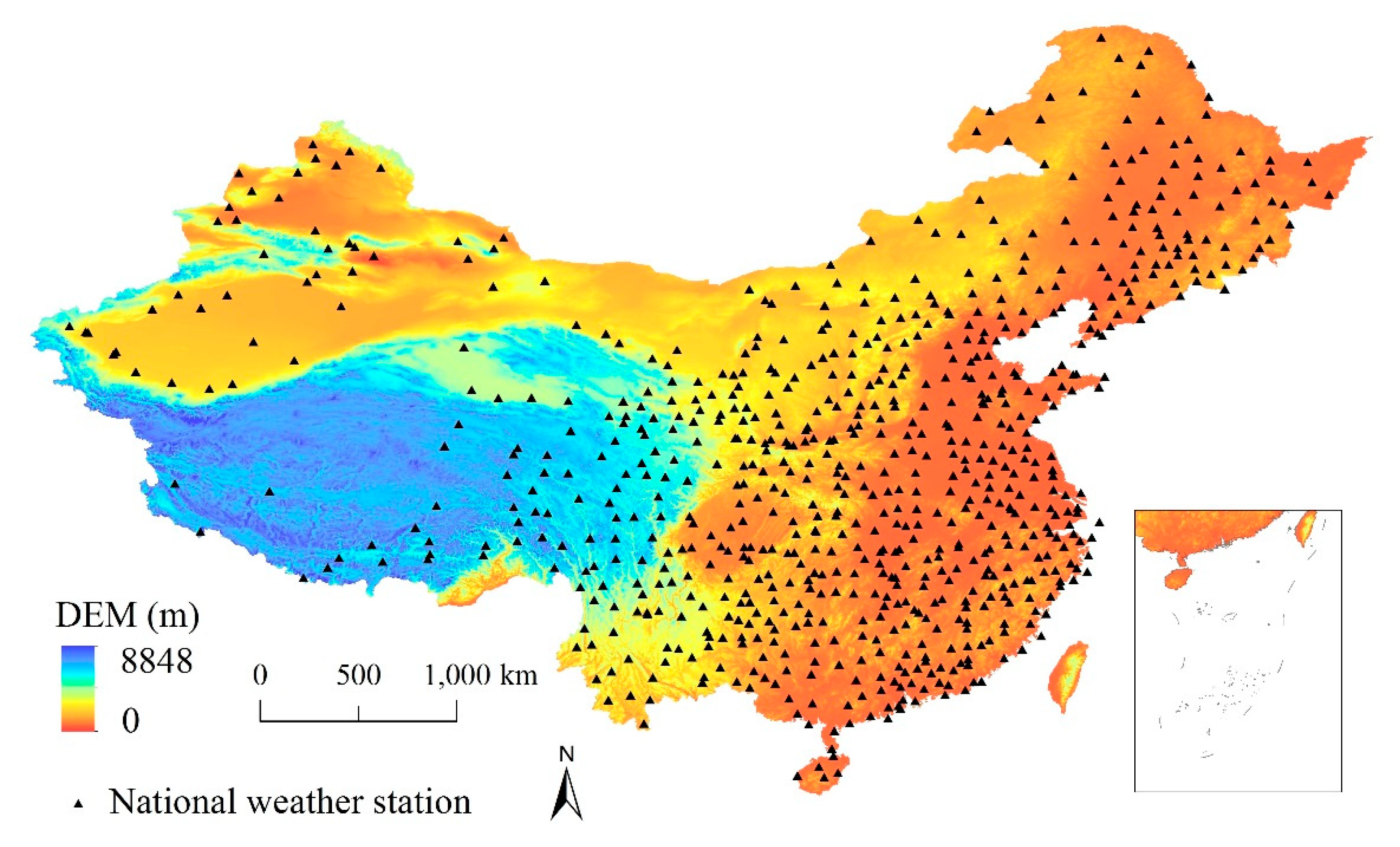
2.1. Data Collection

Climate data with 30 arcmin spatial resolution, including monthly minimum, maximum, and mean temperatures (Tmin, Tmax, and Tmean) and precipitation (PRE) amounts, were obtained from the Climatic Research Unit (CRU, Norwich, UK) TS v. 4.02 dataset [22] and the Coupled Model Intercomparison Project 5 (CMIP5) dataset, projected using 27 general circulation models (GCM) [26]. Currently, the CRU and CMIP5 datasets cover the periods 1901–2017 and 2018–2100, respectively. To downscale these datasets to higher spatial resolutions, a 0.5 arcmin reference dataset was obtained from the WorldClim v. 2.0 dataset [29]. The reference dataset contains the averages of monthly data for the period 1970–2000, generated from 9000–60,000 weather stations around the world using the thin-plate splines interpolation method. The interpolation considered the covariates with elevation, distance to the coast, and three satellite-derived covariates. Thus, this reference dataset includes orographic effects and observed climate information for each month.

Observations of monthly Tmin, Tmax, Tmean, and PRE across China were obtained from the National Meteorological Information Center of China (http://data.cma.cn/en), and were used to evaluate the downscaled temperatures and precipitation. The dataset includes observations of 745 weather stations (Figure 1) for the period 1951–2016.

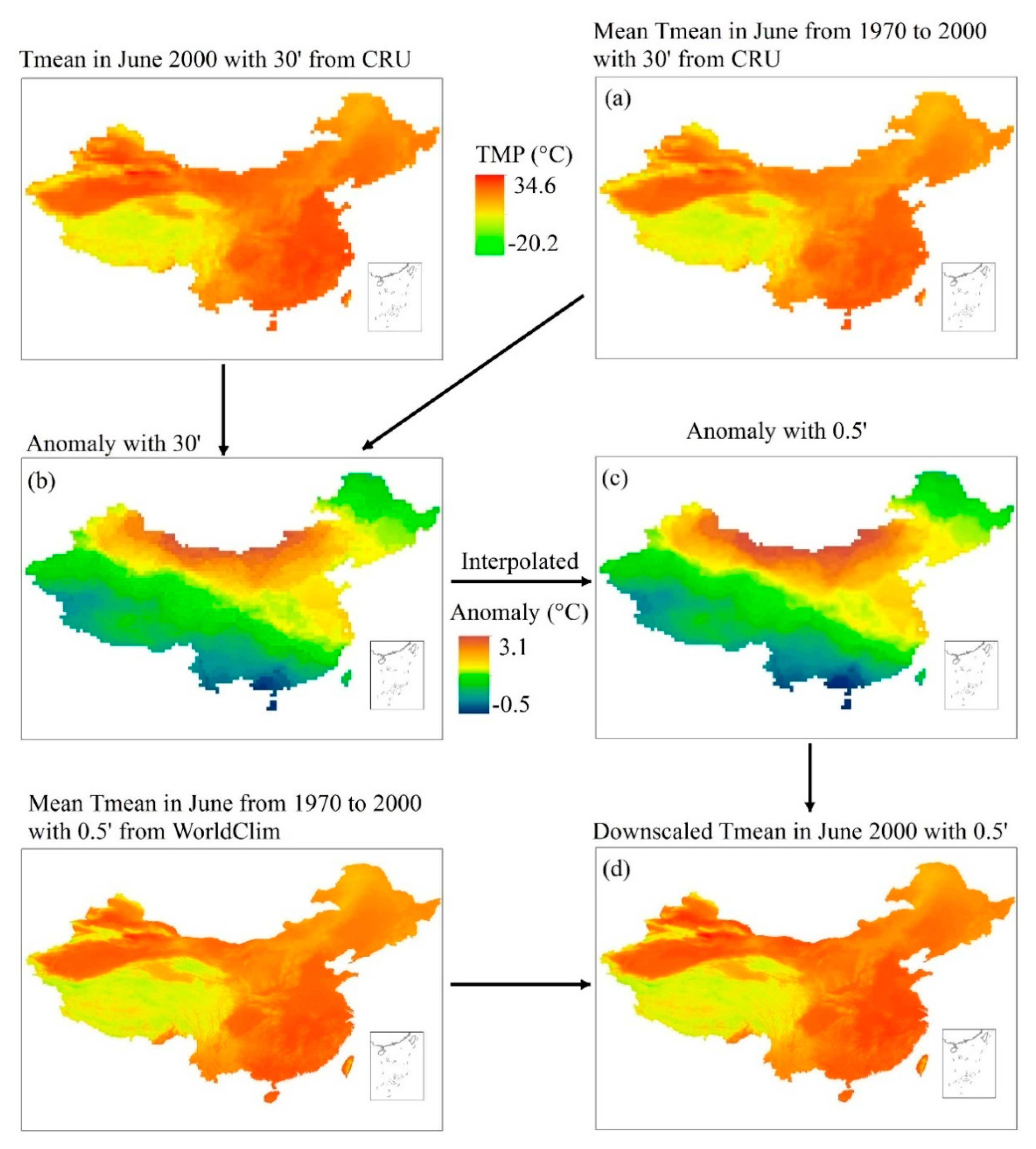
2.2. Spatial Downscaling Method

This study adopted the delta spatial downscaling framework to downscale the 30 arcmin CRU and CMIP5 datasets to a new dataset with 0.5 arcmin resolution across China to bring it to the same resolution as the reference data. Figure 2 illustrates the components and steps of the delta downscaling for Tmean using the 30 arcmin CRU time series and 0.5 arcmin WorldClim climatology datasets. The first step (Figure 2a) involves constructing a 30 arcmin CRU climatology for each month in the period 1970–2000. The second step involves calculating the 30 arcmin anomaly for a specific month relative to the long-term average for that month (Figure 2b). The Tmean anomaly was calculated as the difference between the Tmean in a specific month and the long-term averaged Tmean for that month. The PRE anomaly can be calculated as the ratio of the PRE in a specific month to the long-term averaged PRE for that month. The third step involved spatial interpolation of the 30 arcmin anomaly to the 0.5 arcmin WorldClim grid (Figure 2c). The final step (Figure 2d) involved transformation of the 0.5 arcmin anomaly to the 0.5 arcmin Tmean for that month using the WorldClim climatology for the corresponding month. This transformation reversed the creation of the anomaly; therefore, addition was used for Tmean, while multiplication was used for PRE. It should be noted that the bilinear interpolation method was applied for the interpolation of the anomaly, which has been found to have good performance in the delta downscaling process [24,28].

The new dataset covers the period 1901–2100, where the dataset in the past period (1901–2017) and future period (2018–2100) was downscaled from the CRU and CMIP5 datasets, respectively. This study adopted three Representative Concentration Pathway (RCP) scenarios, i.e., RCP2.6, RCP4.5, and RCP8.5, for the future data. In addition, the modeled temperatures and precipitation for 1950–2005 from 27 GCMs were also downscaled. These downscaled results were compared with the observations from weather stations to select the best GCMs in projecting temperatures and precipitation. We then downscaled future temperatures and precipitation from the three most accurate GCMs and calculated the SPEI to reduce the uncertainty of future SPEI variations introduced by GCMs.

This study used the mean absolute error (MAE) and the Nash–Sutcliffe efficiency coefficient (NSE) to evaluate the 0.5’ downscaled dataset, using the time-series observations of 745 national weather stations for 1951–2016. Because of the different units of the temperature and precipitation, this study used their averaged NSEs to compare the performances of 27 GCMs.

2.3. SPEI Calculation

Precipitation and potential evapotranspiration (PET) are necessary inputs for calculating SPEI [8]. Several methods can be used to estimate PET, such as the Thornthwaite equation [30], the Hargreaves equation [31], or the Penman–Monteith equation [32]. Beguería et al. [33] reported that, compared with the Thornthwaite equation, the SPEI estimated by the Hargreaves equation is very close to that of the Penman–Monteith equation. Moreover, Hargreaves and Allen (2003) reported that, compared with the Penman–Monteith equation, the Hargreaves equation is more suitable for estimating PET in a dry environment and with a long time step (≥five days) [34]. Therefore, to investigate long-term drought variation across China in a warming environment, this study employed the Hargreaves equation to calculate the PET based on the downscaled temperatures. Detailed information for calculating SPEI can be found in Vicente-Serrano et al. [8] and Beguería et al. [33]. This study used SPEI with a 12 month moisture balance to investigate the annual drought variation. Specifically, the SPEI for December of one year was treated as the annual SPEI.

2.4. Trend Analysis

To detect the magnitude of the SPEI trend and the corresponding statistical significance in the annual SPEI variation, the linear regression between the annual SPEI and the year was calculated. The regression coefficient of SPEI represents the trend during a period, while the p-value of this coefficient represents the trend’s significance, calculated at a 95% confidence level.

2.5. Attribution of SPEI Variation

To attribute the SPEI trend to PRE and PET in a period, we obtained the sensitivity coefficient of SPEI related to the PRE and PET using a differential equation (i.e., ∂SPEI/∂PRE and ∂SPEI/∂PET), which is similar to the attribution of PET for climate variables [35]. Thus, the contribution of SPEI variability to either of these variables could be calculated by multiplying the long-term trend of the variable by its sensitivity coefficient [36]. Accordingly, similarly to PET [37], the total contribution of climate variability to SPEI variation could be calculated using the following differential equation:

$$\frac{dSPEI}{dt}=\frac{\partial SPEI}{\partial PRE}\times \frac{dPRE}{dt}+\frac{\partial SPEI}{\partial PET}\times \frac{dPET}{dt},$$

(1)

where dSPEI/dt is the long-term trend of SPEI variation, and dPRE/dt and dPET/dt are the long-term trends of PRE and PET variations, respectively.

However, because of the complexity involved in calculating SPEI, obtaining the differential of SPEI with respect to PRE or PET is very difficult. Consequently, in this study, we developed an alternative approach to quantifying the contributions of PRE and PET. First, Equation (1) was treated as a linear regression equation, as follows:

$$∆SPEI=a\times ∆PRE+b\times ∆PET,$$

(2)

where ΔSPEI, ΔPRE, and ΔPET are the interannual variations in the time series, and a and b are the regression coefficients—specifically, ∂SPEI/∂PRE and ∂SPEI/∂PET, respectively. Then, according to the interannual variation values of SPEI, PRE, and PET in the time series, a and b could be fitted using Equation (2). Moreover, the R² and the p-value were used to evaluate the performance of the fitting. Finally, the contribution of PRE (or PET) was calculated by multiplying the long-term trend of PRE (or PET) by its ∂SPEI/∂PRE (or ∂SPEI/∂PET) using Equation (1). Furthermore, to evaluate the rationality of this approach, the sum of the contributions of PRE and PET was compared with the actual SPEI trend calculated using the relationship of the annual SPEI and year. Thus, the percentage contribution of each variable was calculated as follows [37]:

$$PC\left(x\right)=\frac{C\left(x\right)}{C\left(PRE\right)+C\left(PET\right)},$$

(3)

where x is the PRE or PET, C(x) is the contribution of x, and PC(x) is the percentage contribution of x.

3. Results

3.1. Evaluation of Downscaled Temperatures and Precipitation

Table 1. Statistic information between raw/downscaled and observed monthly minimum, mean, and maximum temperatures (i.e., Tmin, Tmean, and Tmax, respectively) and precipitation (PRE) using 745 national weather stations during the 1951–2016. This evaluation was carried out for the datasets of the raw/downscaled CRU and 27 general circulation models (GCMs).

	Tmin (°C)				Tmean (°C)				Tmax (°C)				PRE (mm)
	Raw		Downscaled		Raw		Downscaled		Raw		Downscaled		Raw		Downscaled
	MAE	NSE	MAE	NSE	MAE	NSE	MAE	NSE	MAE	NSE	MAE	NSE	MAE	NSE	MAE	NSE
CRU	1.62	0.89	1.14	0.96	1.38	0.87	0.84	0.97	1.88	0.74	1.22	0.92	15.13	0.63	13.60	0.76
ACCESS1.0	2.21	0.86	1.83	0.93	2.11	0.86	1.69	0.94	2.59	0.76	2.26	0.84	29.02	0.12	23.27	0.30
BCC-CSM1.1	2.20	0.86	1.86	0.92	2.11	0.86	1.69	0.93	2.59	0.76	2.29	0.83	28.77	0.13	22.94	0.35
BCC-CSM1.1 (m)	2.20	0.86	1.87	0.92	2.11	0.86	1.69	0.94	2.59	0.76	2.30	0.83	29.27	0.12	23.29	0.30
BNU-ESM	2.19	0.86	1.82	0.93	2.10	0.86	1.67	0.94	2.57	0.77	2.24	0.85	28.52	0.20	22.78	0.40
CanESM2	2.18	0.86	1.81	0.93	2.10	0.86	1.67	0.94	2.58	0.76	2.26	0.84	29.03	0.12	23.12	0.32
CESM1-BGC	2.21	0.86	1.87	0.92	2.13	0.86	1.71	0.93	2.61	0.76	2.30	0.83	29.33	0.12	23.33	0.32
CESM1-CAM5	2.18	0.86	1.81	0.94	2.09	0.86	1.66	0.94	2.58	0.76	2.25	0.84	28.88	0.13	23.03	0.37
CMCC-CM	2.20	0.86	1.84	0.93	2.12	0.86	1.71	0.93	2.60	0.76	2.30	0.82	28.78	0.17	22.88	0.38
CNRM-CM5	2.22	0.86	1.85	0.92	2.13	0.86	1.73	0.92	2.62	0.76	2.31	0.83	29.07	0.13	23.20	0.33
CSIRO-Mk3.6.0	2.20	0.86	1.83	0.93	2.12	0.86	1.71	0.93	2.62	0.76	2.29	0.83	29.07	0.12	23.33	0.28
EC-EARTH	2.20	0.86	1.85	0.92	2.12	0.86	1.71	0.93	2.61	0.76	2.31	0.82	29.26	0.08	23.20	0.32
FIO-ESM	2.21	0.86	1.87	0.92	2.13	0.86	1.71	0.93	2.61	0.76	2.33	0.82	29.13	0.12	23.24	0.32
GFDL-CM3	2.23	0.85	1.85	0.92	2.12	0.86	1.72	0.93	2.60	0.76	2.24	0.85	28.53	0.17	22.84	0.33
GFDL-ESM2G	2.19	0.86	1.82	0.93	2.10	0.86	1.68	0.94	2.58	0.76	2.28	0.83	29.08	0.12	23.24	0.33
GFDL-ESM2M	2.19	0.86	1.81	0.93	2.09	0.86	1.67	0.94	2.56	0.76	2.23	0.84	29.04	0.12	23.12	0.37
GISS-E2-H-CC	2.20	0.86	1.85	0.92	2.12	0.86	1.72	0.92	2.61	0.76	2.29	0.83	28.95	0.13	23.03	0.33
GISS-E2-R	2.20	0.86	1.84	0.92	2.12	0.86	1.70	0.93	2.61	0.76	2.30	0.83	28.87	0.13	22.99	0.35
GISS-E2-R-CC	2.22	0.86	1.83	0.93	2.11	0.86	1.69	0.94	2.58	0.76	2.24	0.85	29.06	0.12	23.32	0.28
HadCM3	2.21	0.86	1.84	0.93	2.13	0.86	1.72	0.93	2.61	0.76	2.28	0.84	29.14	0.13	23.18	0.32
INMCM4	2.22	0.86	1.88	0.92	2.13	0.86	1.72	0.93	2.59	0.76	2.29	0.83	28.95	0.12	23.13	0.35
IPSL-CM5A-LR	2.23	0.86	1.88	0.91	2.13	0.86	1.72	0.92	2.59	0.76	2.28	0.83	29.03	0.12	23.04	0.32
MIROC4h	2.18	0.86	1.83	0.92	2.10	0.86	1.68	0.94	2.59	0.76	2.29	0.84	28.89	0.12	23.05	0.35
MIROC5	2.21	0.86	1.82	0.93	2.12	0.86	1.70	0.93	2.62	0.76	2.25	0.85	29.05	0.12	23.45	0.30
MIROC-ESM	2.23	0.86	1.87	0.92	2.14	0.86	1.74	0.92	2.62	0.76	2.31	0.82	29.26	0.10	23.47	0.28
MIROC-ESM-CHEM	2.23	0.85	1.89	0.91	2.15	0.85	1.75	0.92	2.63	0.76	2.34	0.82	28.85	0.12	23.12	0.32
MRI-CGCM3	2.23	0.86	1.88	0.91	2.15	0.85	1.74	0.92	2.63	0.76	2.31	0.83	29.07	0.15	23.17	0.37
NorESM1-M	2.19	0.86	1.83	0.93	2.10	0.86	1.67	0.94	2.59	0.76	2.26	0.84	29.51	0.08	23.47	0.30

Note: Raw and downscaled values had spatial resolutions of 30′ and 0.5′, respectively. MAE and NSE are the mean absolute error and Nash–Sutcliffe efficiency coefficient, respectively.

compares the raw/downscaled and observed monthly Tmin, Tmax, Tmean, and PRE for 1951–2016. The comparison shows that (1) the downscaled values had lower MAEs and higher NSEs than those of the raw values, (2) downscaled temperatures and PRE from the CRU had better performances than those from the GCMs, and (3) of the 27 GCMs, BNU-ESM, CESM1-CAM5, and GFDL-ESM2M performed best in the prediction of temperatures and PRE. Therefore, the delta downscaling framework is appropriate for use in this study. These data were therefore employed to calculate the annual SPEI from 1901 to 2100.

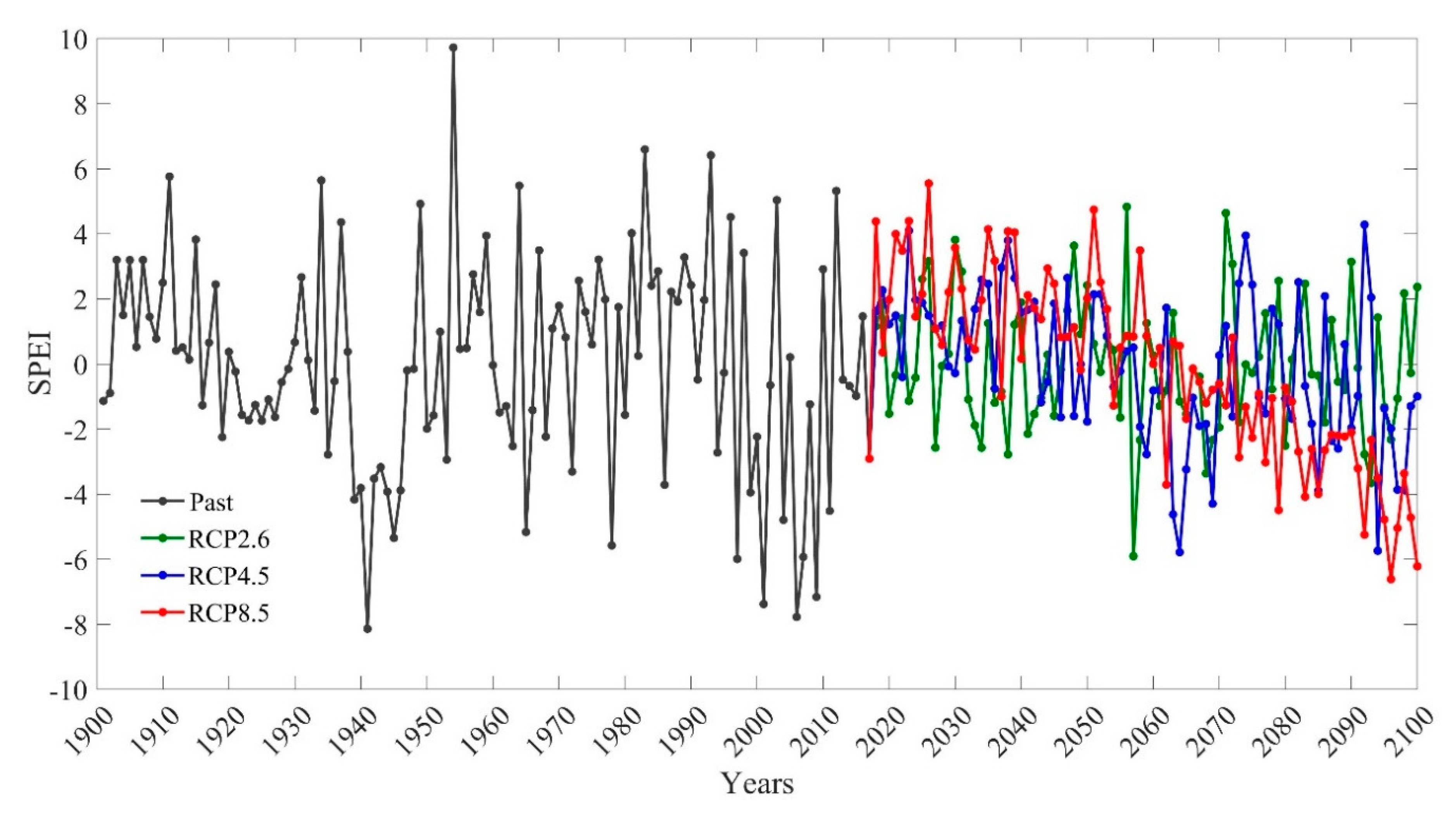
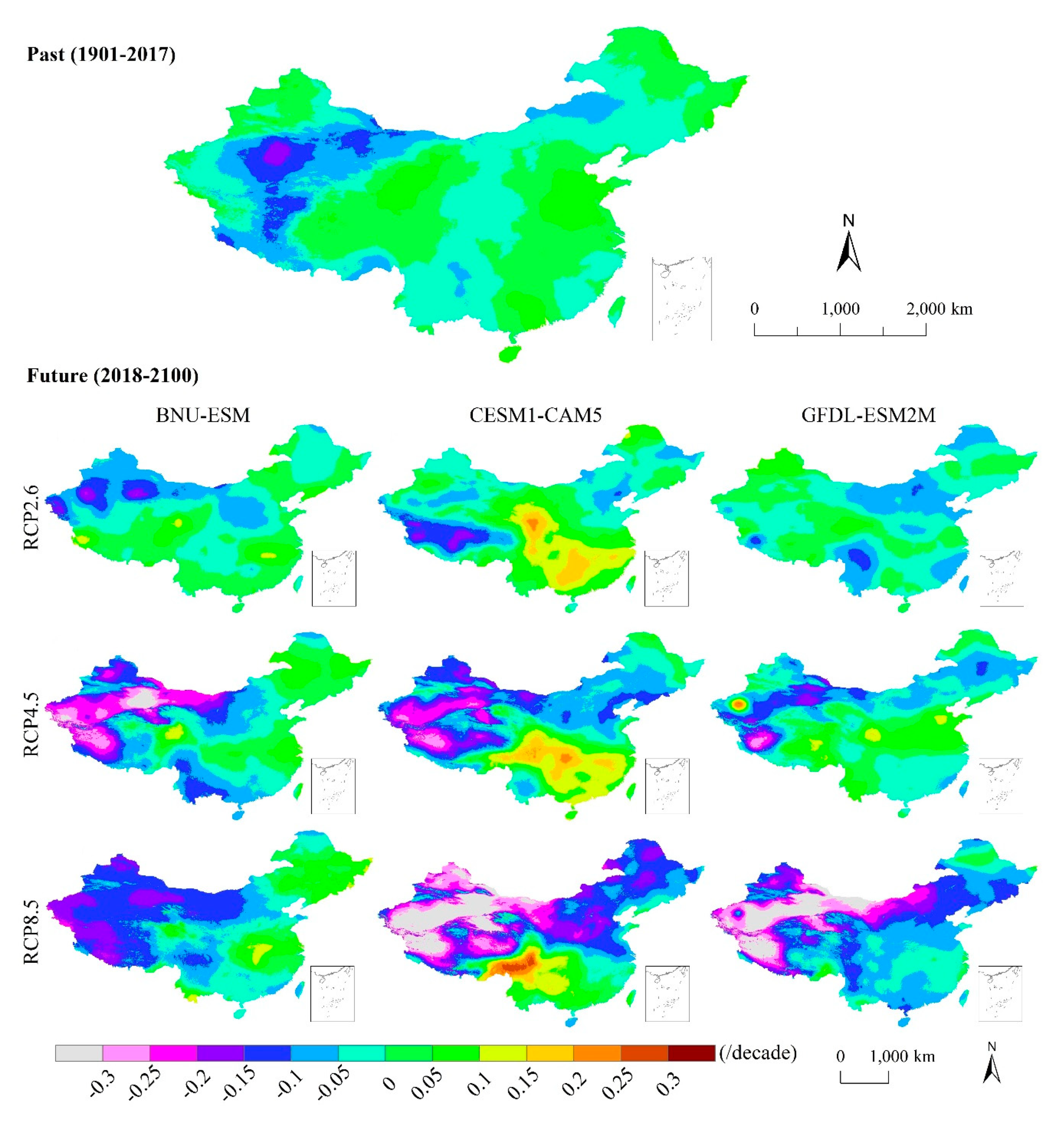
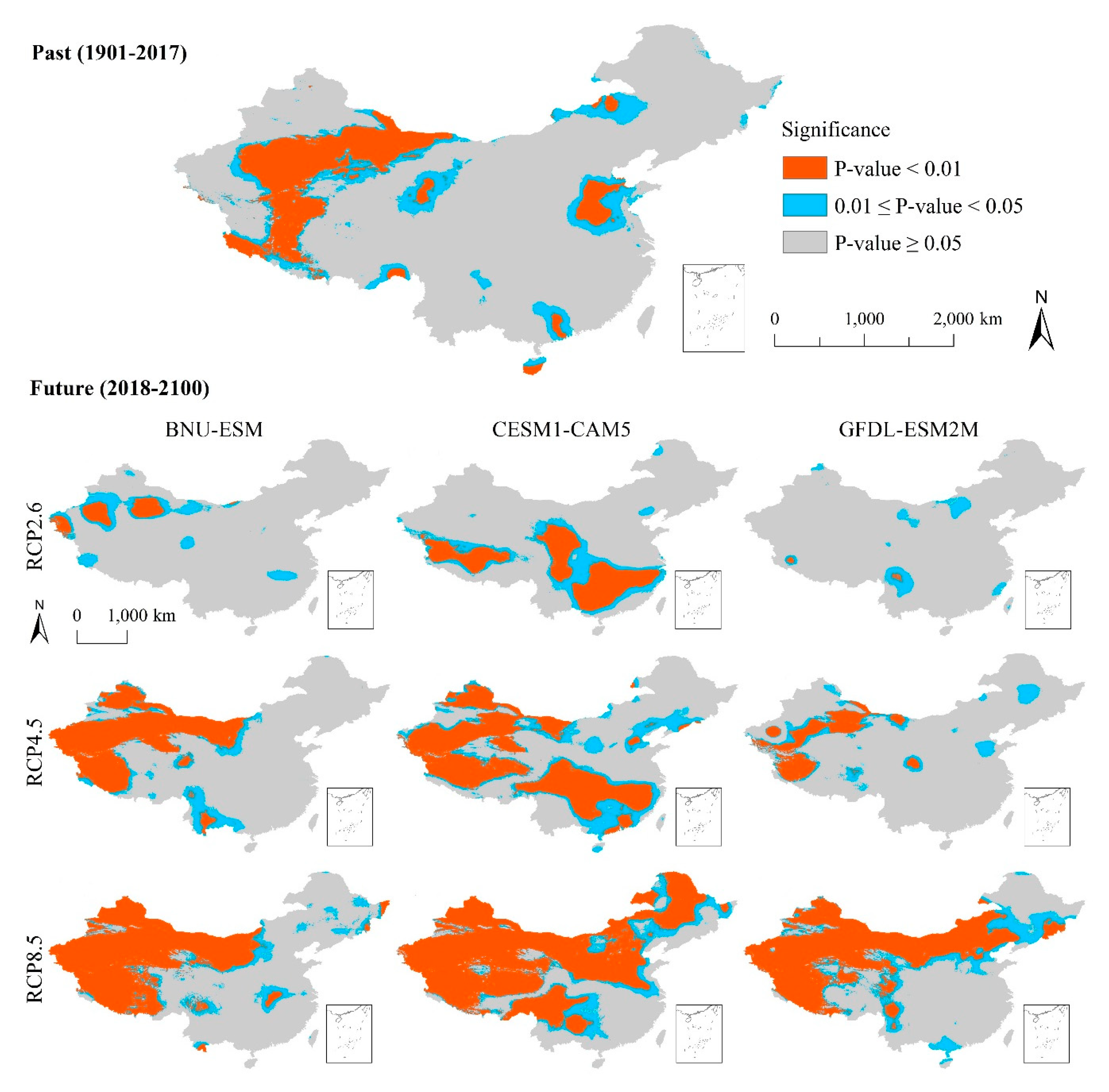
3.2. Spatiotemporal Trends of SPEI

Figure 3 shows the annual SPEI variation from 1901 to 2100 for China. The past SPEI presents a non-significant decreasing trend, whereas the future SPEI exhibits a non-significant decreasing trend under RCP2.6, as well as significant decreasing trends of 0.398/decade under RCP4.5 and 0.969/decade under RCP8.5.

Figure 4 and Figure 5 map the spatial patterns of the trend and the significance of annual SPEI variations during both the retrospective and future periods, while

Table 2. Spatial characteristics of annual SPEI trends (/decade) in the past and future periods.

	1901–2017		2018–2100
			BNU-ESM						CESM1-CAM5						GFDL-ESM2M
			RCP2.6		RCP4.5		RCP8.5		RCP2.6		RCP4.5		RCP8.5		RCP2.6		RCP4.5		RCP8.5
	↓	↑	↓	↑	↓	↑	↓	↑	↓	↑	↓	↑	↓	↑	↓	↑	↓	↑	↓	↑
Min	0.05	0.05	0.09	0.09	0.09	0.09	0.00	0.06	0.09	0.09	0.09	0.09	0.09	0.09	0.09	0.09	0.09	0.09	0.09	0.09
Max	0.17	0.11	0.21	0.13	0.36	0.17	0.27	0.18	0.18	0.23	0.29	0.24	0.38	0.31	0.15	0.11	0.30	0.28	0.38	0.12
Mean	0.09	0.07	0.12	0.10	0.18	0.11	0.13	0.10	0.13	0.13	0.15	0.13	0.20	0.15	0.10	0.09	0.14	0.12	0.19	0.10
Std	0.03	0.01	0.03	0.01	0.07	0.01	0.03	0.02	0.02	0.03	0.05	0.03	0.08	0.05	0.01	0.00	0.04	0.03	0.08	0.01
CV (%)	29.63	11.65	21.78	6.52	36.13	11.86	23.06	17.62	17.95	21.28	31.80	22.33	40.55	36.32	9.81	3.01	30.12	27.79	43.87	8.16
PA (%)	16.70	6.15	9.08	1.86	33.60	0.82	45.34	3.79	7.63	19.70	32.57	19.14	62.17	9.94	4.13	0.22	13.02	2.89	53.58	0.04

Note: Min, Max, Mean, Std, CV, and PA represent the minimum, maximum, mean, standard deviation, coefficient of variation, and percent area, respectively. ↓ and ↑ indicate significant decreasing and increasing trends at 95% significance level, respectively.

lists the corresponding minimum (Min), maximum (Max), mean (Mean), standard deviation (Std), coefficient of variation (CV), and percent area (PA) of the zones with significant trends across China. Overall, the spatial magnitude and significance of the annual SPEI trends varied with the study periods, RCP scenarios, and GCMs. Moreover, the PA of the significantly downward trends was far greater than that of the upward trends for each period and GCM, except for the future trend from CESM1-CAM5 under RCP2.6. Specifically, for 1901–2017, significant decreasing and increasing trends were detected, with means of 0.09 and 0.07/decade, accounting for PAs of 16.70% and 6.15%, respectively. Based on the mean of the trends from the three most accurate GCMs, 2018–2100 had areas of both significant decreasing and increasing trends, with means of 0.12 ± 0.02 and 0.11 ± 0.02/decade under RCP2.6, 0.16 ± 0.02 and 0.12 ± 0.01/decade under RCP4.5, and 0.17 ± 0.04 and 0.12 ± 0.03/decade under RCP8.5. In addition, they accounted for PAs of 6.95% ± 2.54% and 7.26% ± 10.80% under RCP2.6, 26.40% ± 11.60% and 7.62% ± 10.03% under RCP4.5, and 53.70% ± 8.42% and 4.59% ± 5.00% under RCP8.5, respectively.

The CV indicated that the GFDL-ESM2M under RCP2.6 and RCP8.5 showed the smallest and largest spatial variations (3.01% and 43.87%), representing upward and downward trends, respectively. The difference between the maximum and the minimum indicated that the most extreme (0.29/decade) and moderate (0.02/decade) spatial variations were detected in RCP8.5 from CESM1-CAM5 and RCP2.6 from GFDL-ESM2M, respectively. In addition, the spatial patterns of the annual SPEI trends and their significance in future sub-periods (i.e., 23 year and 30 year spans) are presented in Figures S1–S6, and the corresponding statistics are listed in Tables S1–S3. The significant trends during these sub-periods also exhibit strong spatiotemporal variations.

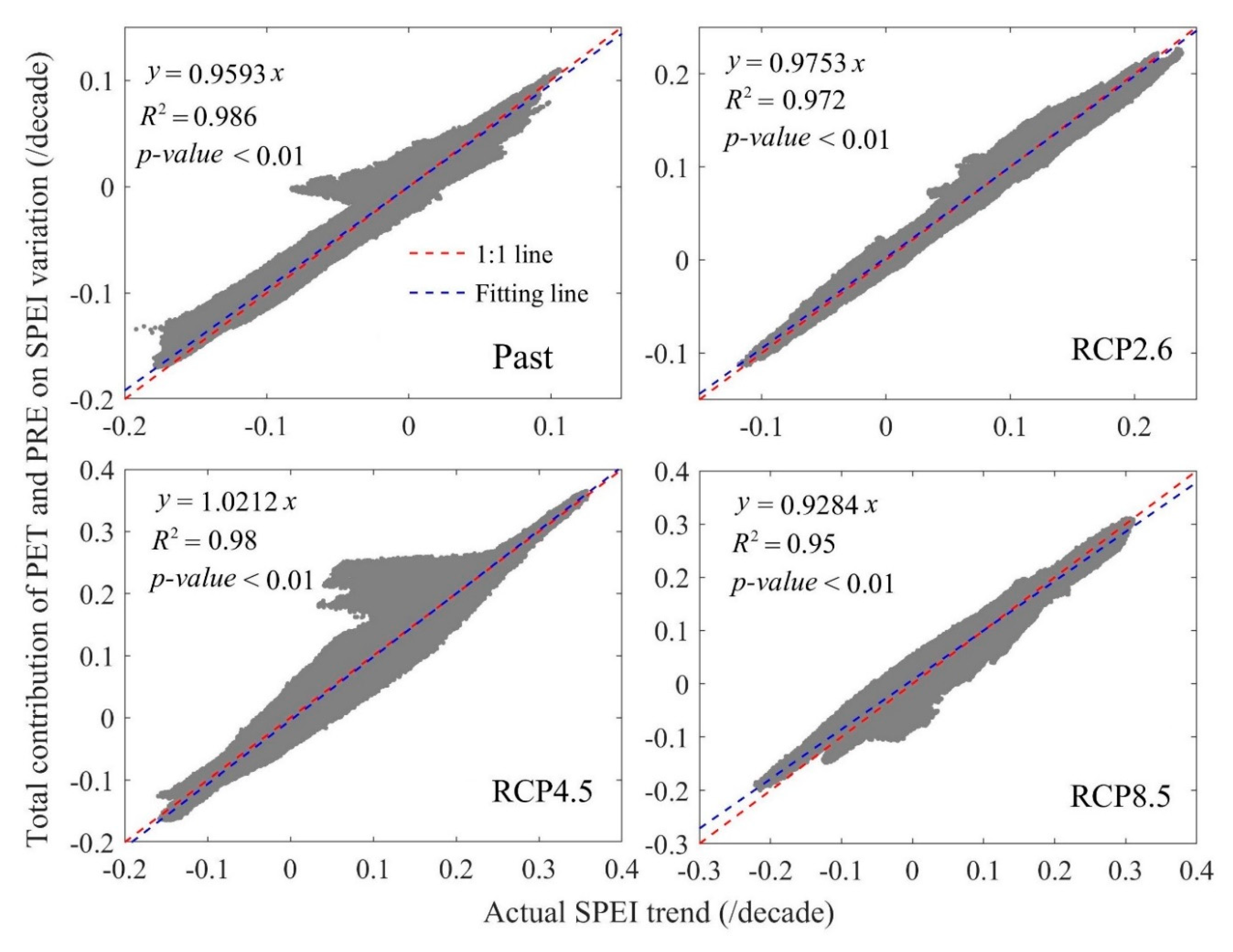
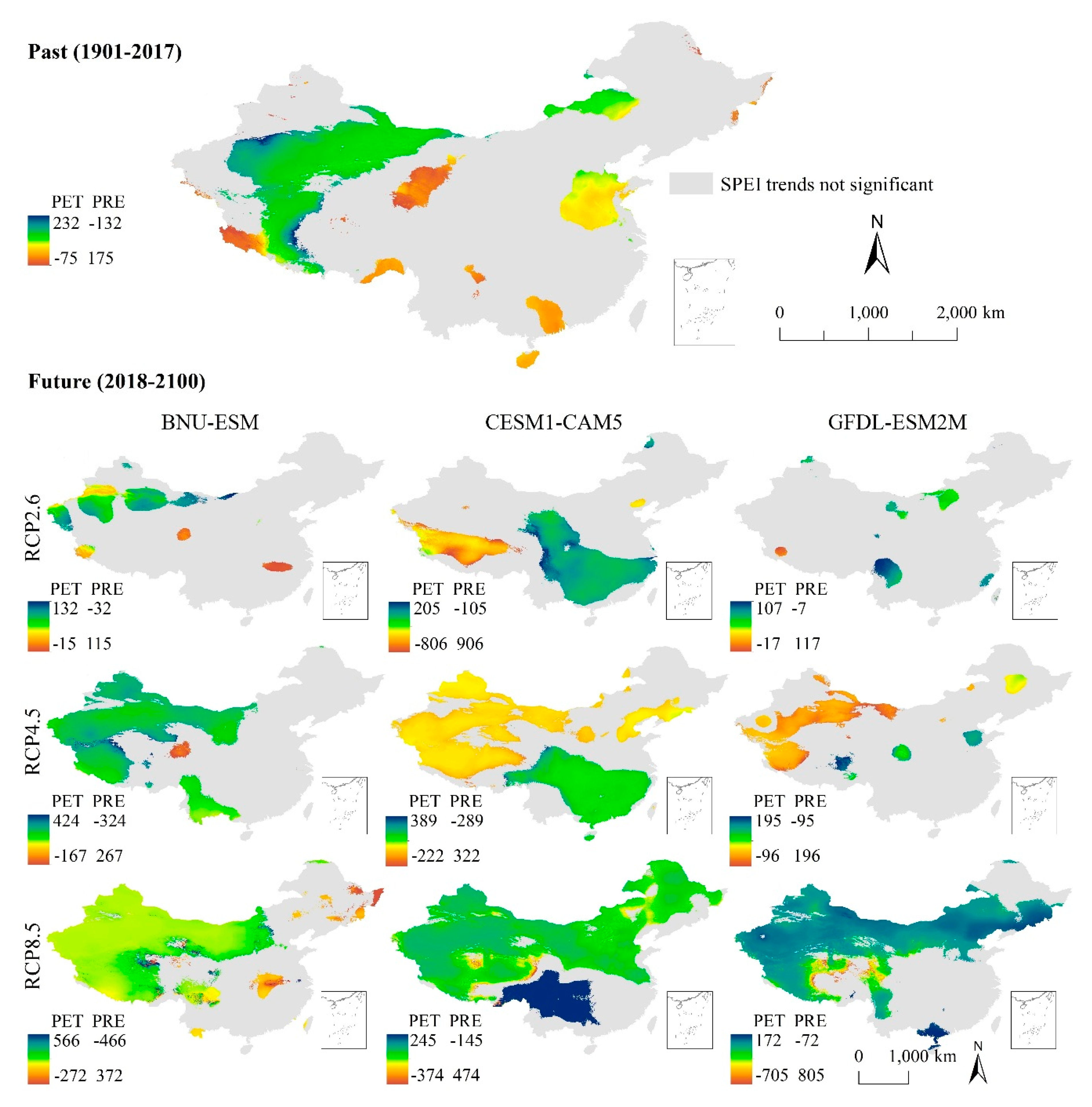
3.3. Attribution of SPEI Variation

Before determining the contributions of PET and PRE to the SPEI variability, the linear regression relationship of their interannual variations expressed using Equation (2) was evaluated (Figure S7). The determination coefficient (R²) and p-value at each grid across China suggested that Equation (2) is a good fit for the data and that the SPEI variation could be completely separated into the PET and PRE variations. The contributions of PET or PRE were calculated based on the regression coefficients at each grid point. Figure 6 shows the comparison between the actual SPEI trends and the total contributions of PET and PRE to SPEI variability during the past and future periods across China. The statistic result showed that the total contribution is very close to the actual SPEI trends, suggesting that this approach to calculating the PET and PRE contributions to SPEI variability is reasonable.

Figure 7 maps the spatial patterns of percentage contributions of PET and PRE to significant SPEI trends (p-value < 0.05), while

Table 3. Spatial characteristics of averaged percentage contributions (%) of PET and PRE on significant SPEI trends in the past and future periods.

	1901–2017		2018–2100
			RCP2.6		RCP4.5		RCP8.5
	↓	↑	↓	↑	↓	↑	↓	↑
PC(PET)	95	28	57 ± 22	5 ± 27	111 ± 9	−44 ± 42	149 ± 20	−90 ± 58
PC(PRE)	5	72	43 ± 22	95 ± 27	−11 ± 9	144 ± 42	−49 ± 20	190 ± 58

Note: ↓ and ↑ indicate significant SPEI decreasing and increasing trends at 95% significance level, respectively. PC(PET) and PC(PRE) are the percentage contributions of PET and PRE, respectively. The future values are the averages of BNU-ESM, CESM1-CAM5, and GFDL-ESM2M.

lists the corresponding geographic statistic information. The results indicate that (1) the downward and upward trends were dominated by PET and PRE, respectively; (2) PC(PET) for downward trends and PC(PRE) for upward trends in the future period are greater than those in the past period; (3) PC(PET) for downward trends and PC(PRE) for upward trends increased with the increased temperatures that occurred in the higher-emissions scenarios; (4) PC(PET) for downward trends was greater than PC(PRE) for upward trends in the past period, while the PC(PET) was less than the PC(PRE) in the future period; and (5) as emissions and global temperatures increased, the PC(PET) for upward trends and PC(PRE) for downward trends became weaker. In addition, their percentage contributions exhibited deep spatial heterogeneity (Figure 7).

4. Summary and Discussion

Although many studies have investigated the SPEI variation over China [12,13,14,15,16,20], little attention has been focused on the detailed spatial variability and attribution of SPEI. This is largely because previous studies employed climate data from low-density stations or low-spatial-resolution reanalysis data, in addition to the computational complexity of differentiation in the equations used to calculate SPEI. This study generated a 1 km resolution monthly climate variable dataset to assess SPEI variability from 1901 to 2100 and developed a simple and reliable approach to differentiating and quantifying the contributions of PET and PRE on SPEI variability. The results could aid the development of sustainable regional and local scale strategies to cope with the adverse effects of global warming and understanding of how global warming affects drought.

This study applied the delta downscaling framework to generate the 1 km resolution monthly climate dataset (Figure 2). The evaluation results suggest that this framework can accurately downscale and correct low-spatial-resolution temperatures and PRE time series (Table 1). Accordingly, detailed spatial patterns and attributions of SPEI variations were mapped across China, and valuable information was detected, such as location and PA. Unlike other studies that adopt geo-statistical interpolation methods (e.g., ordinary kriging and inverse distance-weighted interpolations) to obtain geographic analyses of climate factors [38,39], we could elucidate detailed orographic effects on climate and SPEI variations because of the 1 km reference climatology in the delta downscaling framework. The accuracy of the downscaled temperature dataset was highly dependent on the accuracy of the reference climatology. Although the downscaled dataset was of high quality, there was still a gap between the downscaled data and the observed data. Therefore, a new and better reference climatology should be generated using observed data across China. However, the current publicly available climate data for China are insufficient to construct a reference climatology better than the WorldClim dataset used in this study. In ongoing research, we are devoting efforts to collecting more public and private climate data to construct a better reference climatology dataset and subsequently generate a more accurate downscaled dataset for China.

Compared with past SPEI, the future SPEI has a significant decreasing trend (Figure 3), indicating a greater drought risk. During both past and future periods, significant drought displayed high spatial heterogeneity across China (Figure 4 and Figure 5). The PA of significantly downward trends was far greater than that of upward trends in most cases, especially for northwestern and northern China. These results suggest that an accelerated potential water loss from the surface to the atmosphere in these areas may occur through the end of this century. Therefore, China may see substantially increasing aridity in the future, which will threaten natural vegetation, crop yields, and water resource security. Furthermore, the strong spatial heterogeneity in SPEI trends (Table 2) suggests that detailed adaptation and mitigation strategies should be developed at fine geographic scales.

This study attributed the drought variability to moisture supply and demand based on the SPEI. Thus, the annual SPEI trend was divided between the PET and PRE contributions using Equations (1)–(3). This differs from Cook et al. [1] and Sun et al. [11], who investigated the effects of PET (or PRE) on SPEI anomalies using constant PRE (or PET). Therefore, their investigations could aid understanding of how PET and PRE affect the SPEI fluctuation or magnitude, and this study contributes to understanding the causes of long-term and significant trends in SPEI. According to the calculated percentage contributions, this study first clarified the percentage contributions of PET and PRE to significant SPEI variations for 1901–2017 and 2018–2100 across China. Overall, the results suggest that the percentage contributions vary with study periods, RCP scenarios, directions of trends, and geographic space (Table 3 and Figure 7). The fact that the downward and upward SPEI trends were respectively dominated by PET and PRE conformed to expectations, owing to the definition of SPEI [33]. The future contributions of PET (PRE) on downward (upward) SPEI trends will be greater than the past, which should be attributed to the fact that the future temperature and precipitation over China will be greater and more extreme than the past [18,40]. These quantified contributions of PET (PRE) on significant SPEI trends are beneficial for planning targeted strategies to cope with the adverse effects of drought.

Owing to the complexity involved in calculating SPEI, this study adopted the alternative approach to quantifying the contributions of PRE and PET. The proposed approach performed well according to the evaluations (Figure S7 and Figure 6), and could be used in other regions. However, there is a slight gap between the total contributions calculated by this approach and the actual SPEI trends (Figure 6). This gap is attributable to the fact that the proposed approach does not employ the actual differential method to determine the SPEI. This may limit the accuracy of this approach. Furthermore, this approach focuses on the attribution of annual SPEI trends. However, according to its introduction, this approach has the potential to be expanded to the intra-annual scale, such as monthly, weekly, and daily scale. This expansion depends on the calculation of SPEI and the results of fitting, such as Equation (2), at the intra-annual scale.

References

1. Cook, B.I.; Smerdon, J.E.; Seager, R.; Coats, S. Global warming and 21st century drying. Clim. Dyn. 2014, 43, 2607–2627. [Google Scholar] [CrossRef] [Green Version]
2. Chou, C.; Chiang, J.C.H.; Lan, C.-W.; Chung, C.-H.; Liao, Y.-C.; Lee, C.-J. Increase in the range between wet and dry season precipitation. Nat. Geosci. 2013, 6, 263. [Google Scholar] [CrossRef]
3. Cook, B.I.; Ault, T.R.; Smerdon, J.E. Unprecedented 21st century drought risk in the American Southwest and Central Plains. Sci. Adv. 2015, 1, e1400082. [Google Scholar] [CrossRef] [PubMed] [Green Version]
4. Dai, A. Increasing drought under global warming in observations and models. Nat. Clim. Chang. 2012, 3, 52. [Google Scholar] [CrossRef]
5. Piao, S.; Ciais, P.; Huang, Y.; Shen, Z.; Peng, S.; Li, J.; Zhou, L.; Liu, H.; Ma, Y.; Ding, Y.; et al. The impacts of climate change on water resources and agriculture in China. Nature 2010, 467, 43. [Google Scholar] [CrossRef]
6. McKee, T.B.; Doesken, N.J.; Kleist, J. The relationship of drought frequency and duration to time scales. In Proceedings of the Eighth Conference on Applied Climatology, Anaheim, CA, USA, 17–22 January 1993; pp. 179–184. [Google Scholar]
7. Palmer, W.C. Meteorological drought. Res. Pap. 1965, 45, 1–58. [Google Scholar]
8. Vicente-Serrano, S.M.; Beguería, S.; López-Moreno, J.I. A multiscalar drought index sensitive to global warming: The Standardized Precipitation Evapotranspiration Index. J. Clim. 2010, 23, 1696–1718. [Google Scholar] [CrossRef] [Green Version]
9. Vicente-Serrano, S.M.; Gouveia, C.; Camarero, J.J.; Beguería, S.; Trigo, R.; López-Moreno, J.I.; Azorín-Molina, C.; Pasho, E.; Lorenzo-Lacruz, J.; Revuelto, J.; et al. Response of vegetation to drought time-scales across global land biomes. Proc. Natl. Acad. Sci. USA 2013, 110, 52–57. [Google Scholar] [CrossRef] [Green Version]
10. Vicente-Serrano, S.M.; Camarero, J.J.; Azorin-Molina, C. Diverse responses of forest growth to drought time–scales in the Northern Hemisphere. Glob. Ecol. Biogeogr. 2014, 23, 1019–1030. [Google Scholar] [CrossRef] [Green Version]
11. Sun, S.; Chen, H.; Li, J.; Wei, J.; Wang, G.; Sun, G.; Hua, W.; Zhou, S.; Deng, P. Dependence of 3-month Standardized Precipitation-Evapotranspiration Index dryness/wetness sensitivity on climatological precipitation over southwest China. Int. J. Clim. 2018, 38, 4568–4578. [Google Scholar] [CrossRef]
12. Li, X.; You, Q.L.; Ren, G.Y.; Wang, S.Y.; Zhang, Y.Q.; Yang, J.L.; Zheng, G.F. Concurrent droughts and hot extremes in northwest China from 1961 to 2017. Int. J. Clim. 2019, 39, 2186–2196. [Google Scholar] [CrossRef]
13. Liu, Z.P.; Wang, Y.Q.; Shao, M.G.; Jia, X.X.; Li, X.L. Spatiotemporal analysis of multiscalar drought characteristics across the Loess Plateau of China. J. Hydrol. 2016, 534, 281–299. [Google Scholar] [CrossRef]
14. Zhang, R.; Chen, Z.Y.; Xu, L.J.; Ou, C.Q. Meteorological drought forecasting based on a statistical model with machine learning techniques in Shaanxi province, China. Sci. Total. Environ. 2019, 665, 338–346. [Google Scholar] [CrossRef] [PubMed]
15. Gao, X.R.; Zhao, Q.; Zhao, X.N.; Wu, P.T.; Pan, W.X.; Gao, X.D.; Sun, M. Temporal and spatial evolution of the standardized precipitation evapotranspiration index (SPEI) in the Loess Plateau under climate change from 2001 to 2050. Sci. Total. Environ. 2017, 595, 191–200. [Google Scholar] [CrossRef]
16. Gu, L.; Chen, J.; Xu, C.-Y.; Kim, J.-S.; Chen, H.; Xia, J.; Zhang, L. The contribution of internal climate variability to climate change impacts on droughts. Sci. Total. Environ. 2019, 684, 229–246. [Google Scholar] [CrossRef]
17. Kimosop, P. Characterization of drought in the Kerio Valley Basin, Kenya using the Standardized Precipitation Evapotranspiration Index: 1960–2016. Singap. J. Trop. Geogr. 2019, 40, 239–256. [Google Scholar] [CrossRef]
18. Naumann, G.; Alfieri, L.; Wyser, K.; Mentaschi, L.; Betts, R.A.; Carrao, H.; Spinoni, J.; Vogt, J.; Feyen, L. Global changes in drought conditions under different levels of warming. Geophys. Res. Lett. 2018, 45, 3285–3296. [Google Scholar] [CrossRef]
19. Shiru, M.S.; Shahid, S.; Chung, E.S.; Alias, N. Changing characteristics of meteorological droughts in Nigeria during 1901–2010. Atmos. Res. 2019, 223, 60–73. [Google Scholar] [CrossRef]
20. Wang, Y.F.; Liu, G.X.; Guo, E.L. Spatial distribution and temporal variation of drought in Inner Mongolia during 1901–2014 using Standardized Precipitation Evapotranspiration Index. Sci. Total. Environ. 2019, 654, 850–862. [Google Scholar] [CrossRef]
21. Gao, L.; Wei, J.; Wang, L.; Bernhardt, M.; Schulz, K.; Chen, X. A high-resolution air temperature data set for the Chinese Tian Shan in 1979–2016. Earth Syst. Sci. Data 2018, 10, 2097–2114. [Google Scholar] [CrossRef] [Green Version]
22. Harris, I.; Jones, P.; Osborn, T.; Lister, D. Updated high–resolution grids of monthly climatic observations–the CRU TS3.10 Dataset. Int. J. Clim. 2014, 34, 623–642. [Google Scholar] [CrossRef] [Green Version]
23. Giorgi, F.; Jones, C.; Asrar, G.R. Addressing climate information needs at the regional level: The CORDEX framework. World Meteorol. Org. Bull. 2009, 58, 175–183. [Google Scholar]
24. Peng, S.; Gang, C.; Cao, Y.; Chen, Y. Assessment of climate change trends over the Loess Plateau in China from 1901 to 2100. Int. J. Clim. 2018, 38, 2250–2264. [Google Scholar] [CrossRef]
25. Peng, S.; Yu, K.; Li, Z.; Wen, Z.; Zhang, C. Integrating potential natural vegetation and habitat suitability into revegetation programs for sustainable ecosystems under future climate change. Agric. For. Meteorol. 2019, 269–270, 270–284. [Google Scholar] [CrossRef]
26. Brekke, L.; Thrasher, B.; Maurer, E.; Pruitt, T. Downscaled CMIP3 and CMIP5 Climate and Hydrology Projections: Release of Downscaled CMIP5 Climate Projections, Comparison with Preceding Information, and Summary of User Needs; US Dept. of the Interior, Bureau of Reclamation, Technical Services Center: Denver, CO, USA, 2013. [Google Scholar]
27. Mosier, T.M.; Hill, D.F.; Sharp, K.V. 30-Arcsecond monthly climate surfaces with global land coverage. Int. J. Clim. 2014, 34, 2175–2188. [Google Scholar] [CrossRef]
28. Peng, S.; Ding, Y.; Wen, Z.; Chen, Y.; Cao, Y.; Ren, J. Spatiotemporal change and trend analysis of potential evapotranspiration over the Loess Plateau of China during 2011–2100. Agric. For. Meteorol. 2017, 233, 183–194. [Google Scholar] [CrossRef] [Green Version]
29. Fick, S.E.; Hijmans, R.J. WorldClim 2: New 1-km spatial resolution climate surfaces for global land areas. Int. J. Clim. 2017, 37, 4302–4315. [Google Scholar] [CrossRef]
30. Thornthwaite, C.W. An approach toward a rational classification of climate. Geogr. Rev. 1948, 38, 55–94. [Google Scholar] [CrossRef]
31. Hargreaves, G.H.; Samani, Z.A. Reference crop evapotranspiration from temperature. Appl. Eng. Agric. 1985, 1, 96–99. [Google Scholar] [CrossRef]
32. Allen, R.G.; Pereira, L.S.; Raes, D.; Smith, M. Crop evapotranspiration-Guidelines for computing crop water requirements-FAO Irrigation and drainage paper 56. FAO Rome 1998, 300, D05109. [Google Scholar]
33. Beguería, S.; Vicente-Serrano, S.M.; Reig, F.; Latorre, B. Standardized precipitation evapotranspiration index (SPEI) revisited: Parameter fitting, evapotranspiration models, tools, datasets and drought monitoring. Int. J. Clim. 2014, 34, 3001–3023. [Google Scholar] [CrossRef] [Green Version]
34. Hargreaves, G.H.; Allen, R.G. History and evaluation of Hargreaves evapotranspiration equation. J. Irrig. Drain. Eng. 2003, 129, 53–63. [Google Scholar] [CrossRef]
35. Ning, L.; Bradley, R.S. NAO and PNA influences on winter temperature and precipitation over the eastern United States in CMIP5 GCMs. Clim. Dyn. 2016, 46, 1257–1276. [Google Scholar] [CrossRef]
36. Ning, T.; Li, Z.; Liu, W.; Han, X. Evolution of potential evapotranspiration in the northern Loess Plateau of China: Recent trends and climatic drivers. Int. J. Clim. 2016, 36, 4019–4028. [Google Scholar] [CrossRef]
37. Zheng, H.; Liu, X.; Liu, C.; Dai, X.; Zhu, R. Assessing contributions to panevaporation trends in Haihe River Basin, China. J. Geophys. Res. Atmos. 2009, 114, D24105. [Google Scholar] [CrossRef] [Green Version]
38. Atta-ur-Rahman; Dawood, M. Spatio-statistical analysis of temperature fluctuation using Mann–Kendall and Sen’s slope approach. Clim. Dyn. 2017, 48, 783–797. [Google Scholar] [CrossRef]
39. Li, Z.; Zheng, F.-L.; Liu, W.-Z. Spatiotemporal characteristics of reference evapotranspiration during 1961–2009 and its projected changes during 2011–2099 on the Loess Plateau of China. Agric. For. Meteorol. 2012, 154, 147–155. [Google Scholar] [CrossRef]
40. Chen, L.; Frauenfeld, O.W. A comprehensive evaluation of precipitation simulations over China based on CMIP5 multimodel ensemble projections. J. Geophys. Res. 2014, 119, 5767–5786. [Google Scholar] [CrossRef]
Figure 1. National weather stations across China.
Sustainability 12 00477 g001
Figure 2. Illustration of delta downscaling, taking the mean temperature (Tmean) in June 2000 from the Climatic Research Unit (CRU) as an example. (a)—Mean Tmean in June from 1970 to 2000 with 30′ from CRU, (b)—Anomaly with 30′, (c)—Anomaly with 0.5′, (d)—Downscaled Tmean in June 2000 with 0.5′.
Sustainability 12 00477 g002
Figure 3. Annual SPEI changes during the past (1901–2017) and future (2018–2100) periods. The future trajectory under each RCP scenario is the averaged result of BNU-ESM, CESM1-CAM5, and GFDL-ESM2M.
Sustainability 12 00477 g003
Figure 4. Spatial patterns of trends in annual SPEI variations during past (1901–2017) and future (2018–2100) periods.
Sustainability 12 00477 g004
Figure 5. Spatial patterns of trend significance in annual SPEI variations during past (1901–2017) and future (2018–2100) periods.
Sustainability 12 00477 g005
Figure 6. Comparison between the actual SPEI trends (x) and the total contribution of potential evapotranspiration (PET) and PRE on SPEI variations (y) for past (1901–2017) and future (2018–2100) periods across China. The total contribution under each RCP scenario is the averaged result of BNU-ESM, CESM1-CAM5, and GFDL-ESM2M.
Sustainability 12 00477 g006
Figure 7. Spatial patterns of percentage contributions (%) of PET and PRE on significant SPEI trends (p-value < 0.05) for past (1901–2017) and future (2018–2100) periods.
Sustainability 12 00477 g007