Spatiotemporal Patterns and Drivers of the Surface Urban Heat Island in 36 Major Cities in China: A Comparison of Two Different Methods for Delineating Rural Areas

Abstract

Urban heat islands (UHIs) are an important issue in urban sustainability, and the standardized calculation of surface urban heat island (SUHI) intensity has been a common concern of researchers in the past. In this study, we used the administrative borders (AB) method and an optimized simplified urban-extent (OSUE) algorithm to calculate the surface urban heat island intensity from 2001 to 2017 for 36 major cities in mainland China by using Moderate Resolution Imaging Spectroradiometer (MODIS) images. The spatiotemporal differences between these two methods were analyzed from the perspectives of the regional and national patterns and the daily, monthly, and annual trends. Regardless of the spatial or temporal scale, the calculation results of these two methods showed extremely similar patterns, especially for the daytime. However, when the calculated SUHI intensities were investigated through a regression analysis with multiple driving factors, we found that, although natural conditions were the main drivers for both methods, the anthropogenic factors obtained from statistical data (population and gross domestic product) were more correlated with the SUHI intensity from the AB method. This trend was probably caused by the spatial extent of the statistical data, which aligned more closely with the rural extent in the AB method. This study not only explores the standardization of the calculation of urban heat intensity but also provides insights into the relationship between urban development and the SUHI.

1. Introduction

In 2014, over 54% of people in the world lived in densely populated urban areas, and it is expected that the global urban population will increase to 66% of the total population by 2050 [1]. Rapid urbanization is one of the most important human influences on the atmosphere and causes obvious disruptions of atmospheric energy [2,3]. The most widely known consequence of these influences is the generation of the urban heat island effect. The urban heat island concept was first proposed by Howard in 1833 [4], and it is used to describe the phenomenon where the temperature of an urban area is higher than that of the surrounding rural area. In the past several decades, a large number of scholars have studied the damage that urban heat islands bring to the natural environment and human life, including reducing biodiversity [5], destroying vegetation growth [6], reducing the quality of air and water [7], changing the climate [8,9], and increasing morbidity and mortality [10,11,12]. There is ample evidence that when these effects interact with global changes, the intensity of the impact is further increased [9].

Generally, previous studies have considered two types of urban heat islands: the atmospheric urban heat island (AUHI) and the surface urban heat island (SUHI) [13]. Data on the AUHI are generally obtained from the analysis of in situ air temperatures from weather stations [8]. However, the number of weather stations is low, which results in a low observation density, and they are unevenly distributed [11]. It is, therefore, difficult to obtain the spatial distribution of the AUHI for large areas. Conversely, remote sensing technology can periodically obtain comprehensive coverage of land surface temperatures (LSTs). Since the first analysis on the SUHI by Rao in 1972 [14], many scholars have conducted research on the SUHI, based on thermal infrared remote sensing data [15,16,17,18,19,20,21,22].

As the SUHI intensity is simple, efficient and universal, it has become the most common indicator for researching the SUHI [23,24]. The principle for estimating the SUHI intensity is to find an urban-rural pair and then calculate the temperature difference between the urban and rural areas. Therefore, the core problem for calculating SUHI intensity is delineating urban and rural areas [18]. Most studies have adopted a relatively consistent approach for identifying urban areas: the areas classified as built-up land in land cover maps are considered urban areas [13,25,26,27]. For the determination of rural areas, it is generally assumed that all areas within a certain range around the urban area are rural; thus, the determination of the rural area extent has been an important issue. In past studies, the most common methods were to set a buffer zone at a certain distance (CD), such as 1–50 km [13,19,28,29,30,31], or to set a buffer zone based on the size of the urban area (SUA), such as 0.5–3 times the area of the urban area [18,32,33,34]. However, regardless of which method is adopted, there is no widely recognized standard method.

The standardization of urban heat island intensity calculations is a scientific issue of great value, and considerable work has been performed on this topic. Schwarz et al. [35] first compared the temperature differences between core-rural areas and urban-other areas, which then became a milestone for remote sensing studies of the SUHI [36]. At the global scale, Clinton and Gong [19] found that the SUHI intensity became larger as the rural buffer became larger. Zhou et al. [32] estimated that the footprint of the UHI effect can reach 2.3 and 3.9 times more than the urban area size in, respectively, daytime and nighttime, with large spatiotemporal heterogeneities. Li et al. [13] characterized the significances and spatiotemporal dynamics of rural-extent-induced SUHI intensity variations in mainland China, and they found that differences in rural definitions may lead to significant uncertainties in the studies of SUHI intensity. Zhou et al. [36] proposed that large uncertainties associated with the definitions of urban areas and its references have been one of the most urgent issues in UHI studies.

According to previous studies, the current calculation method for SUHI intensity has the following problems. (1) It is not appropriate to simply adopt a buffer radius, especially in the case of the simultaneous investigation of multiple cities with different geographical locations and different levels of socioeconomic development [27]. (2) Choosing different rural extents will result in a larger or even opposite difference in the calculation results. For example, Peng et al. [18] defined the nearby suburbs as rural reference areas and found that the global average summer SUHI intensities for daytime and nighttime were 1.9 °C and 1.0 °C, respectively, while Zhang et al. [20] used the 20 km surrounding buffer zone as the extent of the rural area and obtained daytime and nighttime SUHI intensities of 2.6 °C and 1.6 °C, respectively. This limitation impedes the accurate characterization of the spatiotemporal patterns of the SUHI intensity and distorts the comparability between previous studies. (3) Although some studies have analyzed the relationship between the SUHI intensity obtained from a certain size buffer and the various statistical data obtained from administrative districts, this strategy is also inappropriate [37,38] due to the differing spatial extents of the two data representations.

Compared with the CD and the SUA, adopting an appropriate fixed boundary (FB) for the rural area can solve the above problems to some extent. Lai et al. [27] employed the groundbreaking administrative borders (AB) method to determine the extent of rural areas and explored the typical diurnal patterns of the surface urban heat islands in China. Chakraborty and Lee [25] proposed the simplified urban-extent (SUE) algorithm based on the urban area data provided by Natural Earth and compared the results with those of the previous multicity SUHI studies to verify the availability of the algorithm. This comparison was an important step in the process of the standardization of the calculation of SUHI intensity. However, no researchers have analyzed the differences between these two representative fixed boundaries in the existing UHI literature. There is an obvious need to better understand the UHI phenomenon by comparing the differences between these methods for SUHI intensity calculation to help city planners and other researchers make more sensible decisions about the future of urban sustainability.

The objectives of this research were (i) to compare the differences in spatiotemporal patterns of SUHI intensity between the AB and SUE methods in 36 Chinese major cities and (ii) to identify the factors associated with the SUHI intensity by considering a series of social, economic and natural factors with these two methods. Section 2 describes the study area, data and comparison method in this study. Section 3 shows the spatiotemporal patterns and drivers of the SUHI intensity in 36 Chinese cities. Section 4 discusses the results and highlights the notable problems.

2. Materials and Methods

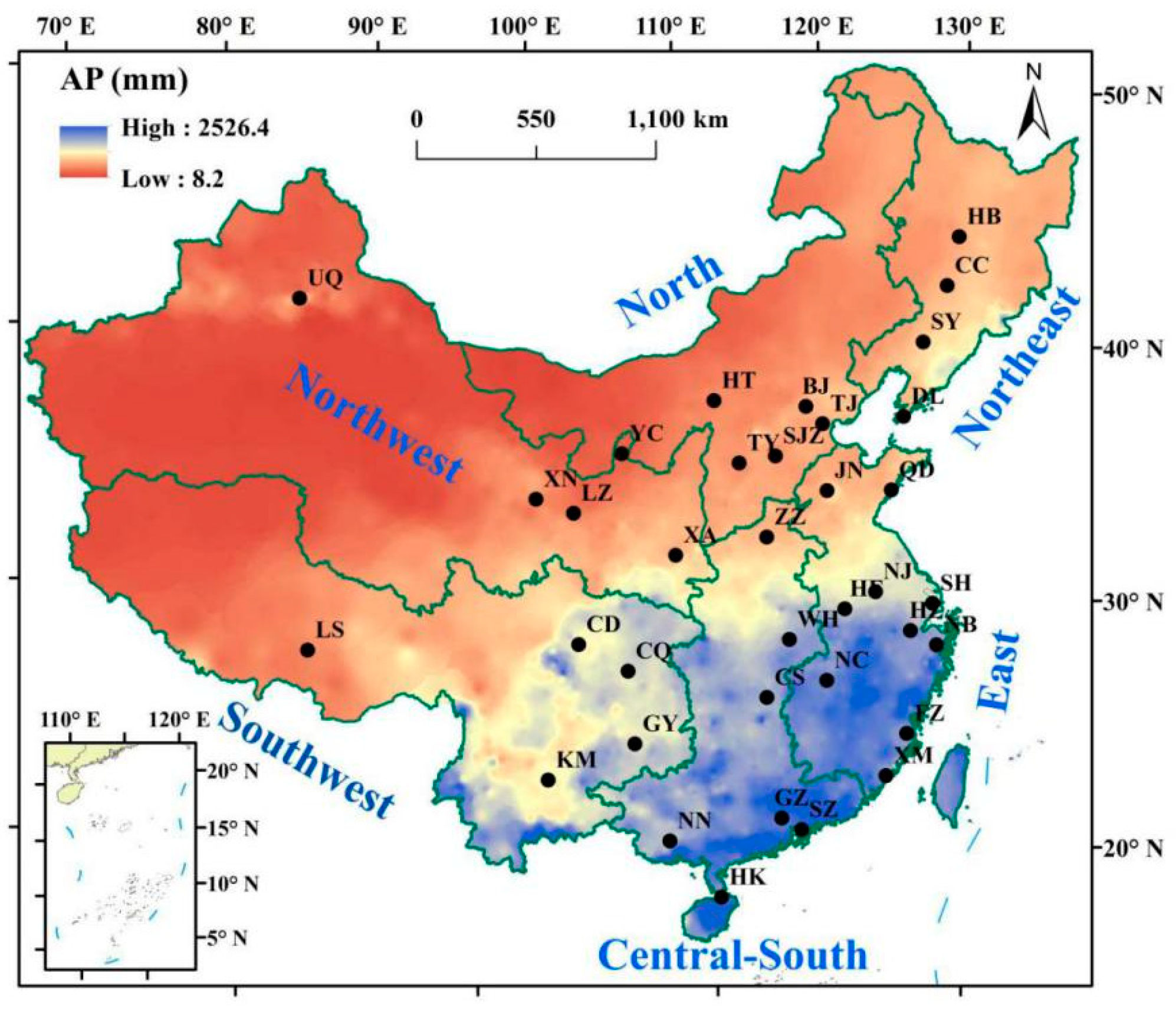
2.1. Study Area

China is a large country located in East Asia that faces the western cost of the Pacific Ocean. Past research shows that there is a large precipitation gradient between Northwest and Southeast China [13], and different levels of the urban heat island (UHI) phenomenon have been observed among different areas in China. In this research, 36 major cities in China were selected as the research areas, and they contain 31 capital cities or direct-controlled municipalities and 5 important port cities (Shenzhen, Ningbo, Xiamen, Qingdao and Dalian). These major cities are the economic (such as Shanghai) or political (such as Beijing) centers of each region and have experienced significant urbanization in the past decade, which deserves further study to determine the associated changes of the UHI effect. The administrative areas of the above 36 cities were defined based on data from the National Geomatics Center of China (NGCC). In addition to studying the differences in SUHI intensity between cities in different regions according to natural conditions, climate conditions and social economic conditions, we divided China into six regions(www.resdc.cn). These 6 regions were the separate northern, northwestern, northeastern, eastern, central-southern and southwestern areas, as shown in Figure 1.

2.2. Data

This paper employed Terra and Aqua Moderate Resolution Imaging Spectroradiometer (MODIS) 8-day composite land surface temperature (LST) products (MOD11A2 and MYD11A2; collection 6 at 1 km × 1 km resolution) from 2001 (the Aqua data is from 2003–2017) to gain the LST. The LST product was retrieved from the clear-sky observations through the generalized split-window LST algorithm [39] at approximately 1:30 (nighttime, Aqua), 10:30 (daytime, Terra), 13:30 (daytime, Aqua) and 22:30 (nighttime, Terra) local solar time. The research of Wan [40] showed that the retrieval errors of MODIS LST were generally <1 k and the root mean square (RMS) was <0.5 k. Wan [41] then pointed out that the mean error of collection for 6 LST datasets was within 0.6 k in 10 validation data samples.

We use the land cover products that were obtained from the MODIS yearly land cover type L3 global 500 m products (MCD12Q1; collection 6 at 500 m × 500 m resolution) from 2001–2017 for the delineation of the urban and rural areas. Derived from MODIS Aqua and Terra, the product is a 17-category classification under the International Geosphere-Biosphere Program (IGBP) scheme. The Normalized Difference Vegetation Index (NDVI) product was obtained from the Aqua MODIS 16-day composite dataset (MYD13Q1, collection 6, at 250 m × 250 m resolution). To match the resolution of the LST, we aggregate the land cover products and NDVI products to 1 km. Similarly, we use the method to find the difference in the enhanced vegetation index (EVI) (ΔEVI), which is a proxy for green vegetation density differences between the urban and rural pixels. The data were obtained from the Aqua 16-day EVI dataset, which is available at the resolution of 250 m × 250 m (MYD13Q1) in the same time span.

To eliminate the influence of the elevation factor on the calculation for the SUHI intensity, we selected NASA Shuttle Radar Topography Mission (SRTM) data provided by the United States Geological Survey (USGS). Previous research has shown that these data have better vertical accuracy than the Global Multiresolution Terrain Elevation Data from 2010 (GMTED2010) and the advanced spaceborne thermal emission and reflection radiometer (ASTER) elevation data [42].

The urban area data (UAD), which were used in the SUE algorithm, were from Natural Earth (www.naturalearthdata.com). Natural Earth is a combination of the global urban land use database [43,44] and the Landscan population database of the Oak Ridge National Laboratory [45]. This dataset has already been validated using a Landsat-based map of 140 urban areas in different ecoregions and for different levels of population and economic development and has an overall accuracy of 93% [44]. More information about these data can be found from www.naturalearthdata.com.

The contributions of anthropogenic activity can be calculated by separately considering the major sources of economic development and human metabolism. This study used statistical datasets of the gross domestic products (GDPs) and populations of 36 major cities from 2001 to 2017, which were available from the National Bureau of Statistics (www.stats.gov.cn). We also collected a spatial interpolation dataset (at 1 km × 1 km resolution) of annual precipitation and annual moisture index from the Resource and Environment Data Cloud Platform (www.resdc.cn).

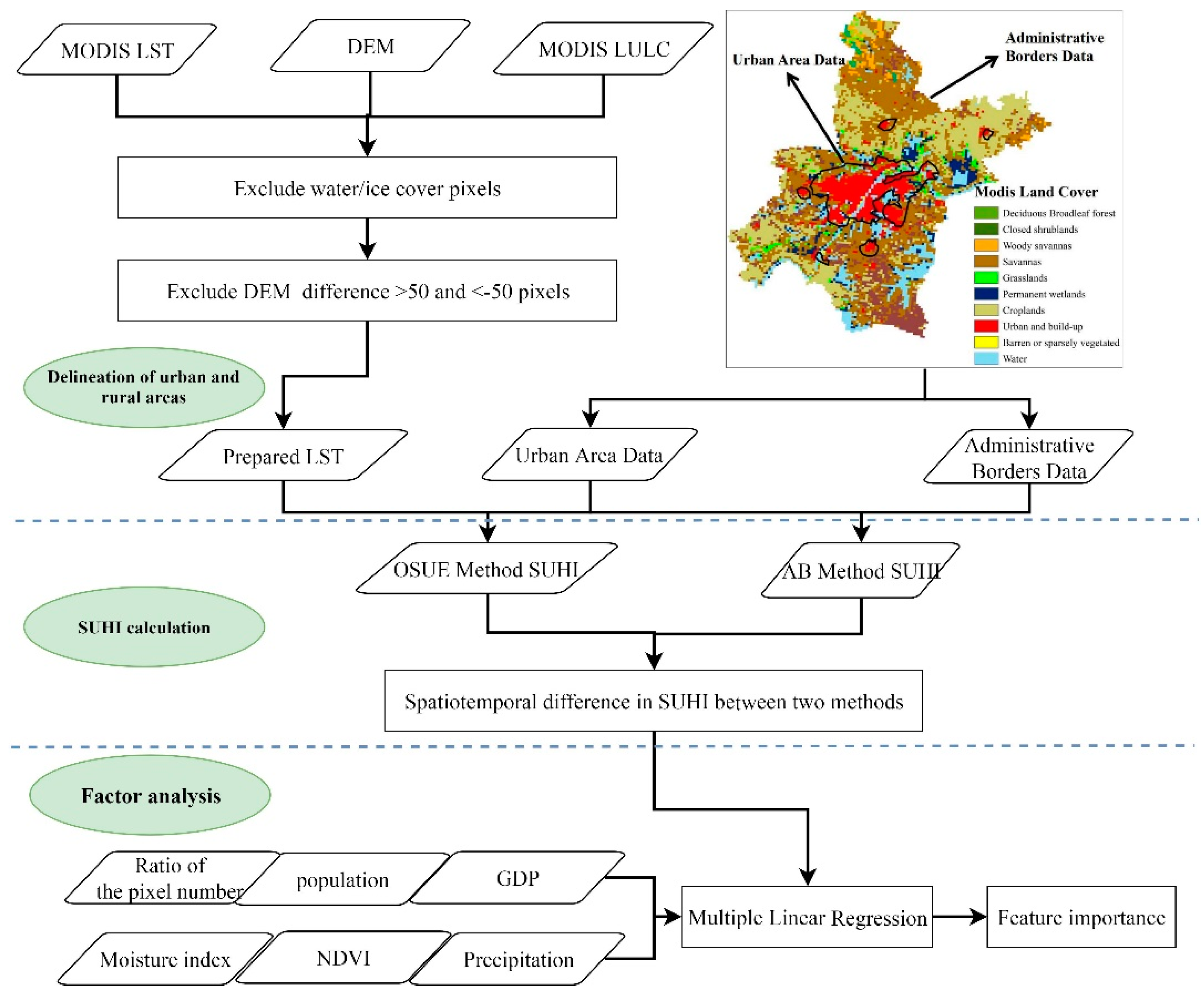
2.3. Method

This research work can be divided into three parts (Figure 2). First, the urban areas and rural areas were delineated with two different methods. Second, the SUE and AB were used to calculate the SUHI intensity of the long time-series data of 36 major cities in mainland China and then to analyze the spatiotemporal differences between the calculation results obtained by the two methods. Third, a correlation analysis was performed between the SUHI and its possible driving factors.

2.3.1. Delineation of Urban and Rural Areas

In this study, we delineated urban and rural areas with the MODIS land cover product MCD12Q1. Within each city, we first removed certain types of pixels: the pixels classified as snow and ice and the pixels in an extremely high or low position (pixels with elevations higher or lower than 50 m than the average of built-up pixels). The removal of those pixels is necessary to eliminate the possible effects of temperature from water bodies and extreme positions. Excluding specific pixels is a common processing method in current SUHI calculations. Yao et al. [46] carefully analyzed the impact of removing these pixels in the SUHI intensity calculation and suggested that these pixels should be removed when calculating the multicity SUHI intensity. For each city with its rural extents, pixels classified as built-up among the remaining pixels were then given a flag as urban areas. Accordingly, we referred to the other pixels after that as rural areas. In this paper, the differences between the two methods (SUE and AB method) may occur based on only the rural area extent. The rural area extents in the SUE method were the largest UAD area within the boundaries of the administrative district of each city. The rural area extents of the AB method were the administrative boundaries of each city (Figure 2). It should be noted that different elevation data are input in the SUE algorithm implemented in this paper, unlike with the original version; therefore, we named it the optimized SUE to differentiate it from the previous method.

2.3.2. Calculation of the SUHI Intensity

After determining the rural area extent of each city with both methods, we first processed the LST image using the MODIS land cover products. We excluded the pixels classified as snow and ice at the beginning due to the possible miscalculation caused by extremely low temperatures. The pixels classified as water or permanent wetlands were also removed to avoid the influence from water temperature. In addition, based on the STRM data, we eliminated pixels in each city that were at elevations of more than ±50 m of that of the built-up pixels to suppress the impact of elevation on the LST. After the above processing, we used Equation (1) to calculate the SUHI intensity as follows:

$$\mathit{SUHI}={\mathit{LST}}_{\mathit{Urban}}-{\mathit{LST}}_{\mathit{Rural}}$$

(1)

where SUHI represents the urban heat island intensity of the city, LST_Urban is the average land surface temperature in the urban area, and LST_Rural is the average temperature of the pixels in the rural area.

To compare the differences in the temporal trends between the AB method and the OSUE method SUHI, we combine the Theil–Sen median trend analysis and the Mann–Kendall test to analyze the calculated results. Theil–Sen median trend analysis is a robust statistical method for trend analysis [42], and it calculates the median slopes between all of the possible n(n − 1)/2 pairwise combinations throughout the time-series data. The method is based on nonparametric statistics and is particularly effective when the estimation of trends in small series is needed [43]. The Mann–Kendall test is applied to measure the significance of a given trend. It is a nonparametric statistical test with an advantage of being irrelevant to the distributions of its samples. The test is also free from the interference of outliers [44]. The effective combination of these two methods is an important method for judging the trends of long-term series data [45].

In this study, we measured the significance of SUHI intensity trends in the daytime and nighttime from 2003–2017 at a confidence level of 0.05. To facilitate the comparison of the differences between the different methods, we divided the trend from all cities into four categories according to the results obtained from the two aforementioned methods (Theil–Sen median trend analysis and the Mann–Kendall test): significant decrease, nonsignificant decrease, significant increase and nonsignificant increase.

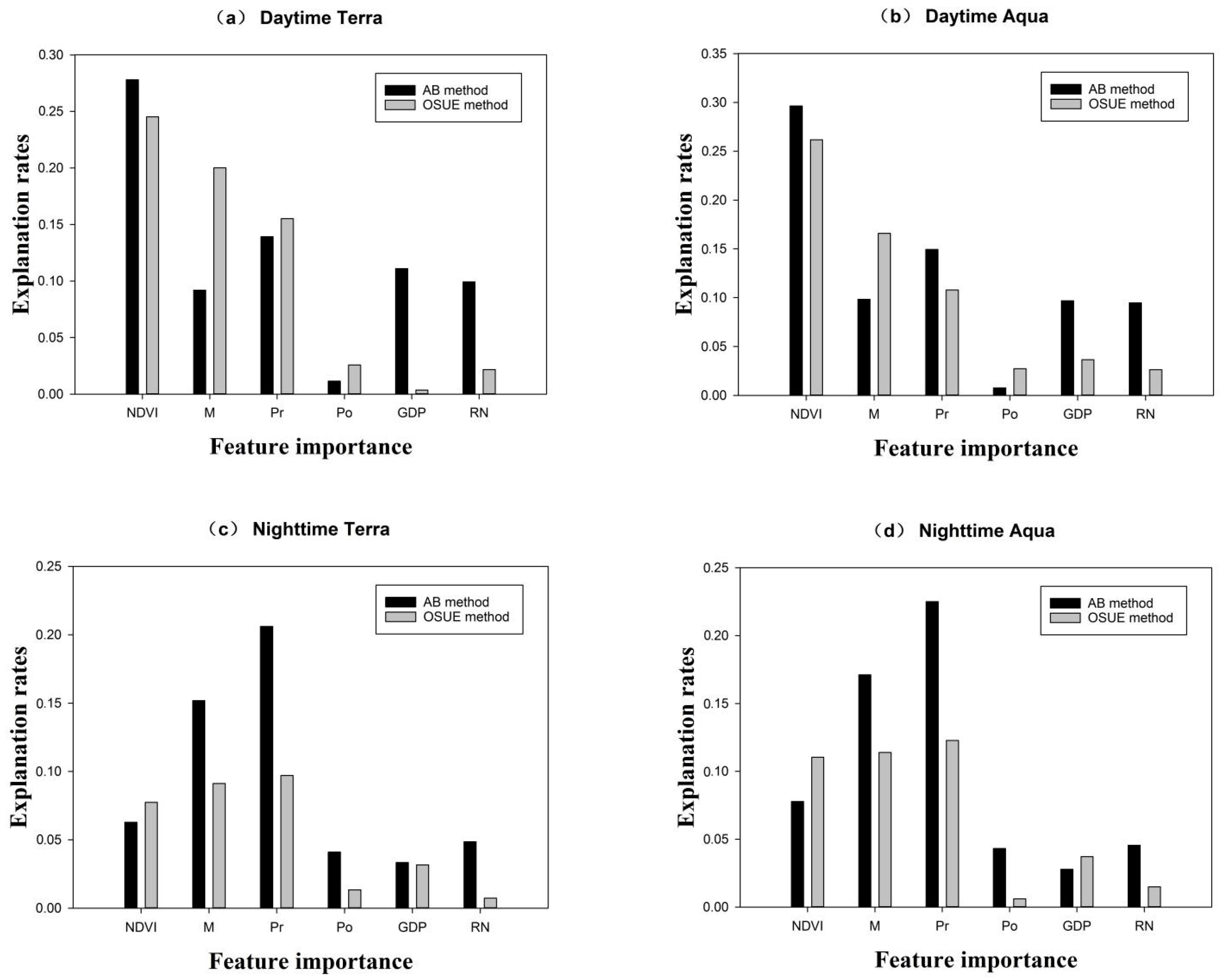
2.3.3. Driving Factor Analysis

In past research, many scholars have studied the influencing factors of SUHI intensity and identified the main driving factors as natural factors, such as the NDVI, EVI, and precipitation, and social factors, such as the population and GDP. Among these factors, the data that characterize the natural conditions are usually raster data obtained by interpolation; and the statistical data that describe the socioeconomic development are mostly annual scale data obtained with the administrative area as the unit. We selected the NDVI, precipitation (Pr), and moisture index (M) to represent these factors specifically, and selected the two most important indicators of urban development level, GDP and population, and analyzed them with the SUHI intensity. In addition, one of the essential differences between the two calculation methods was the difference in the number of pixels between the urban and suburban areas involved in the calculation. To this end, we also defined a new indicator: the ratio of the number of urban pixels to the number of rural pixels involved in the calculation in each city (RN).

3. Results

3.1. Spatial Distribution

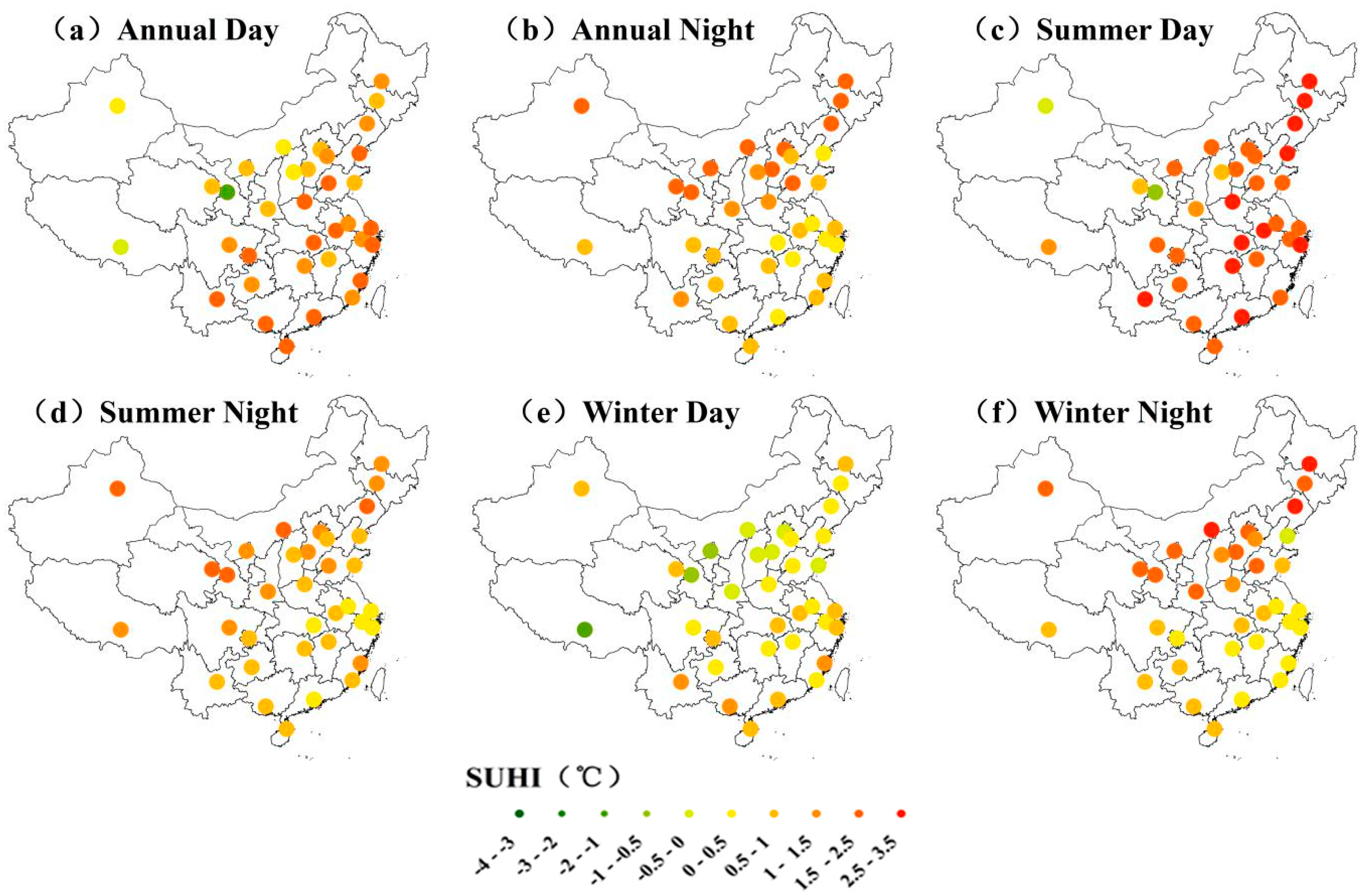
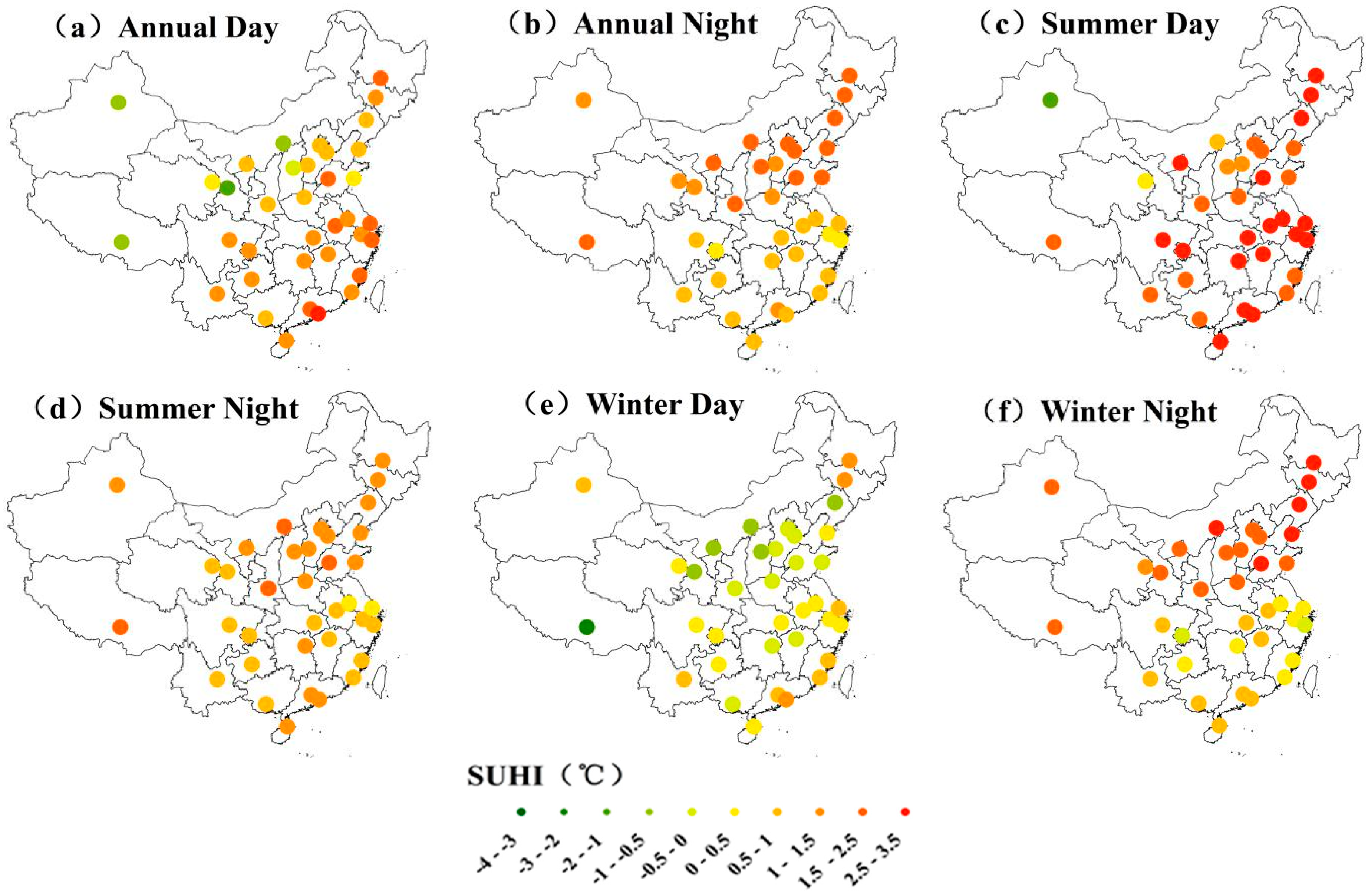
3.1.1. National Patterns

The annual SUHI, summer SUHI and winter SUHI have attracted the most attention from scholars in the past. Therefore, in this study, we also described the daytime and nighttime SUHI in 36 major cities in China (Figure 3 and Figure 4), from 2001 to 2017, for these three conditions to understand the national distribution pattern of SUHI. (As Guangdong and Shenzhen have a high urbanization level and the distribution is centralized, they have been defined as one city in the OSUE method; there are 35 cities in Figure 4.) The daytime and nighttime intensities were consolidated values from the Terra and Aqua platforms.

Most cities had a positive annual daytime SUHI intensity. The AB and OSUE methods identified the proportions of SUHI intensity with positive values at 86% and 94%, respectively. The annual nighttime SUHI intensity values were all positive. The lower annual SUHI intensity values in the daytime were mainly in the northwestern, southwestern and northern areas, and the lower annual SUHI intensity values were distributed in the southeastern and central-southern areas; this distribution was opposite to the trend of the daytime values. The annual daytime SUHI in both methods showed negative values that were significantly lower than the national average level in Lanzhou. Lanzhou is a dry city, and according to the land cover maps, Lanzhou had a large number of pixels classified as the barren land cover type. The occurrence of this urban cold island phenomenon was consistent with the conclusions from the studies of Chakraborty and Lee [25], who indicated that the urban clusters with negative surface UHI were concentrated in the dry and desert areas.

The summer daytime SUHI in both methods was significantly higher than the winter daytime and annual daytime SUHI values. This outcome showed that the SUHI in most cities had an obvious seasonal effect. The winter daytime SUHI in both methods showed obvious differences between the northern and the southern areas, and the SUHI intensity of the northern cities was significantly higher than that of the southern cities. This outcome may be related to the central heating policy in northern China. Most cities in northern China adopt this approach, which significantly enhances the SUHI intensity during winter nights. The daytime winter SUHI intensity from the AB method showed that nearly half of the cities had negative values, while with the OSUE method, only one quarter of cities had negative values. This difference may be related to the fact that the surface temperature of vegetation during the day is higher than that of the buildings in the winter and the AB method usually includes more suburban areas.

3.1.2. Variations across Regions

To further observe the distribution of the annual SUHI intensity in different regions, we calculated the average SUHI intensity for all cities in each region from 2001–2017. It can be seen, from Figure S1, that although there are some differences in the numerical values of SUHI intensity calculated by the two methods, the relative differences between the different regions were basically the same. From the average of each region, the annual daytime SUHI intensity in the northern region was significantly lower than that in the southern region. In the nighttime, except for the northwestern region, the SUHI intensity value calculated by the AB method was higher than that of the OSUE method. The average value of the daytime SUHI intensity in the northwest was the lowest among all regions, although the standard deviation was too large (mainly due to the low SUHI intensity in Lanzhou City during the day). As a result, there was no clear point of reference for this average value. Significant differences within each region can lead to quite high standard error values in many cases. Increasing the number of cities in the study could improve the result to some extent, suggesting that the impact of climate on the SUHI intensity is limited.

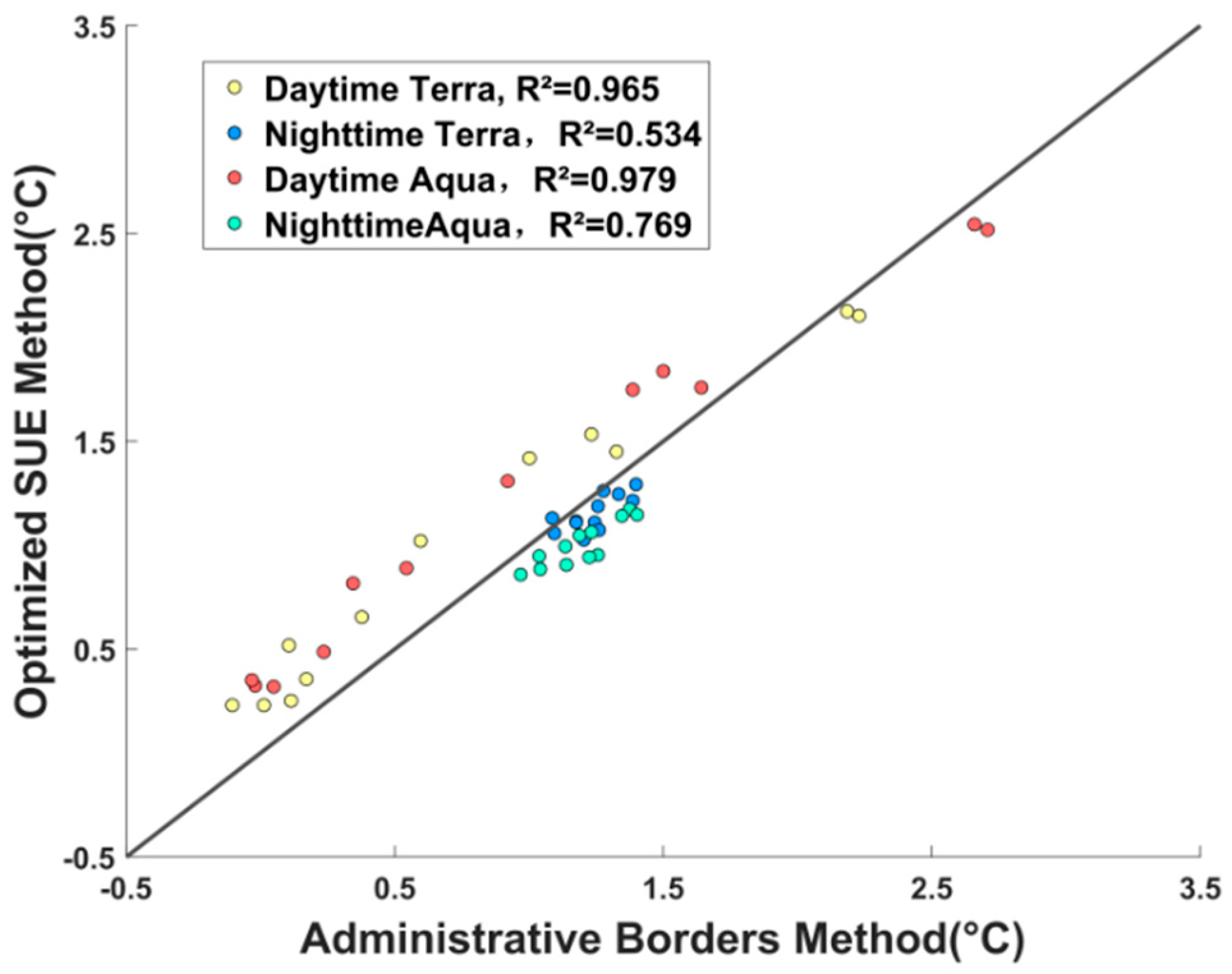
3.1.3. Correlation Analysis of the Annual SUHI

We conducted a correlation analysis of the annual average SUHI intensities of 34 cities calculated by the AB and OSUE methods from 2001–2017 (the SUHI data obtained from the Terra platform was for 2003–2017) to further study the differences between the two methods. Figure 5 shows that the annual daytime SUHI intensity calculated by the two methods had a strong correlation with both the Terra platform and the Aqua platform, with the R² values reaching 0.662 and 0.643, respectively. When the SUHI intensity was low, the OSUE method had a certain degree of overestimation compared to the AB method.

3.2. Temporal Patterns

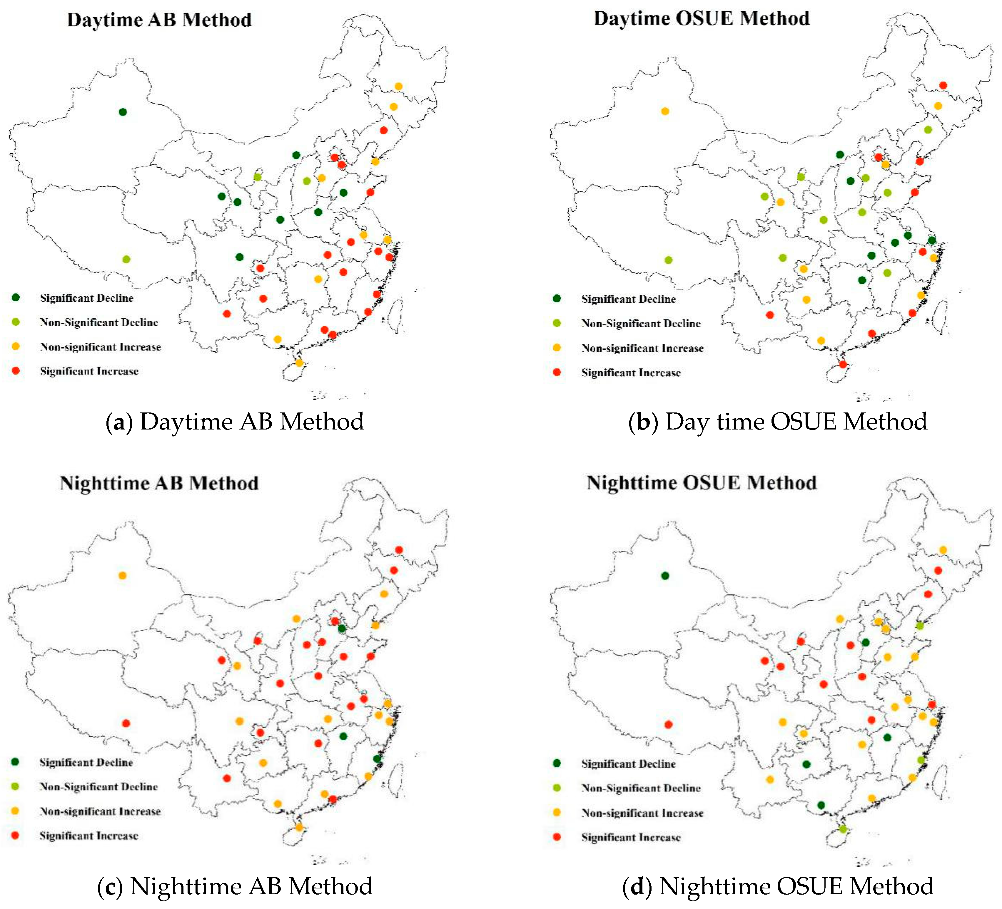
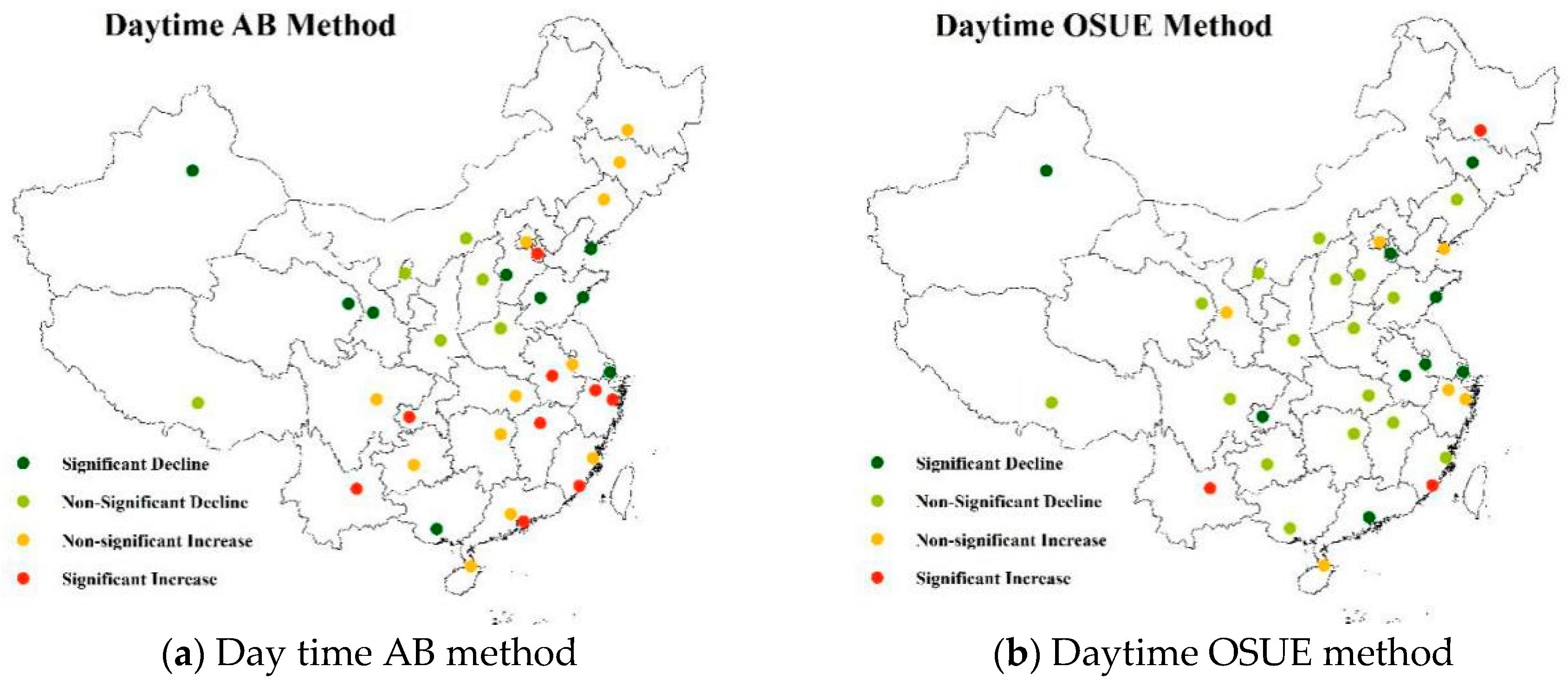
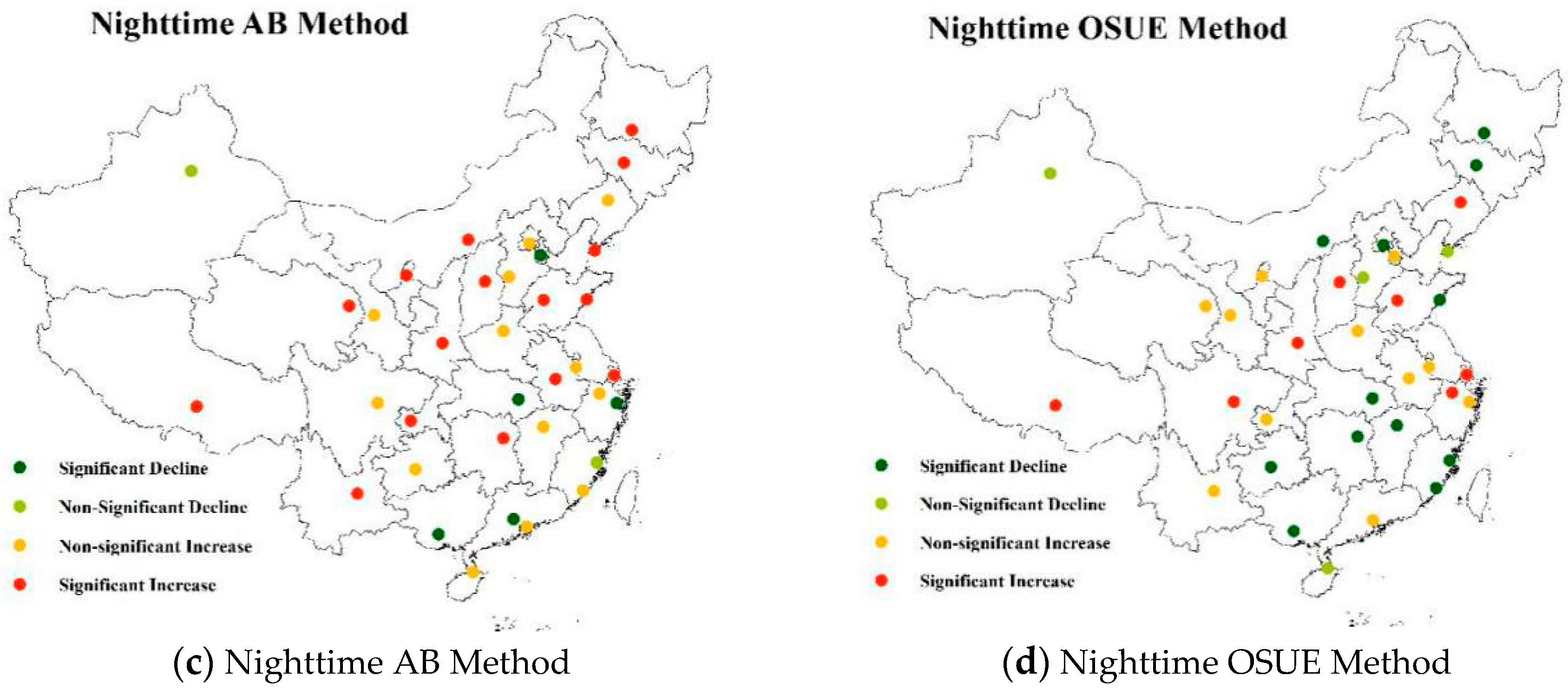
3.2.1. Annual Trend

Figure 6 and Figure 7 show that the calculation results from the two methods had similar variation tendencies in most areas. A completely opposite tendency was observed in the daytime SUHI intensities of Guiyang and Hefei and the nighttime SUHI intensity of Taiyuan with the application of the two methods. In the 34 cities, the proportion of cities with small differences in the daytime SUHI and nighttime SUHI calculated by the two methods was 77.8% and 88.9%, respectively. For these two methods, the cities with different daytime SUHI intensities and nighttime time-varying trends were mainly located in southeastern and northern China, which was primarily related to the variation of the SUHI drivers in northern and southern China.

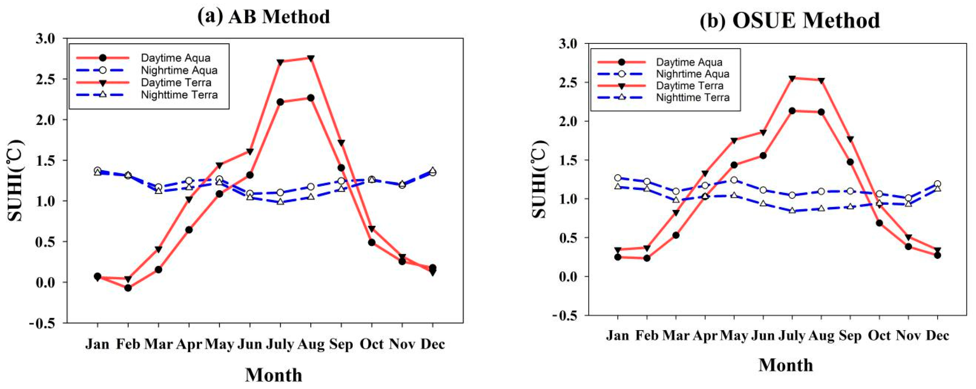
3.2.2. Monthly Trends

The monthly average SUHI intensity for 12 months (one year) is calculated by the two methods and presented in Figure 8. The seasonal variation tendency of SUHI intensity by the two methods is very close. The daytime SUHI intensity is the highest in summer and the lowest in winter. The summer SUHI intensity calculated by the AB method is obviously higher than that calculated by the OSUE method, whereas the winter SUHI intensity calculated by the AB method is slightly lower than that calculated by the OSUE method. The seasonal variations of SUHI intensity are more obvious when applying the OSUE method.

We conducted a correlation analysis to compare the SUHI intensity using the two methods with data obtained from the Aqua and Terra platforms (Figure 9). We found that the daytime monthly average SUHI intensity calculated by the two methods was very close regardless of the platform; the R² values were 0.979 and 0.965 for the daytime Terra and daytime Aqua data, respectively. However, the variation in the nighttime was obvious, and the R² values were 0.769 and 0.534 for the nighttime Terra and nighttime Aqua data, respectively.

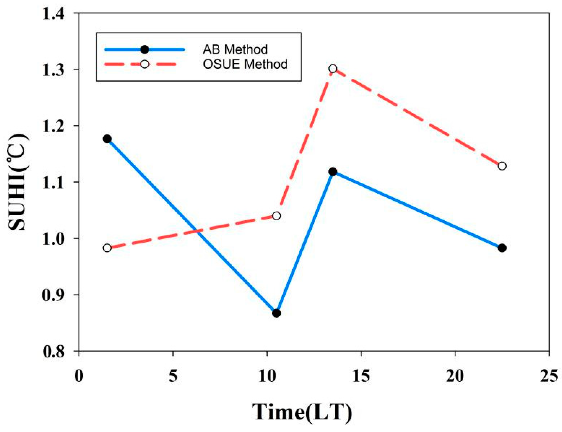
3.2.3. Daily Trends

We analyzed the average values for four different times of day in all Chinese cities based on the two calculation methods. We found that the SUHI intensity calculated by the AB method was slightly higher than that of the OSUE method at 0130 LT, whereas for all other times, the SUHI intensity calculated by the AB method was lower than that by the OSUE method (Figure 10). The strongest surface urban heat island time from the OSUE method within an entire day was similar to the time that had the highest temperature, namely, 1330 LT. However, the strongest urban heat island time was the time with the lowest temperature from the AB method, which was 1330 LT. In addition, in the AB method, the SUHI intensity reached its maximum value at approximately 01:30, and it was slightly higher (about 0.058 °C) than at 13:30. This outcome may have occurred because the rural area pixels occupied a high proportion in the AB method and the temperature of the barren land in rural areas decreases rapidly in nighttime, resulting in the high nighttime SUHI intensity from the AB method.

In general, the driving factors of the SUHI intensity with these two methods were quite different, especially those related to social development, which suggested that the SUHI calculated by the AB method may be better able to help people study the social development factors that cause the UHI effect.

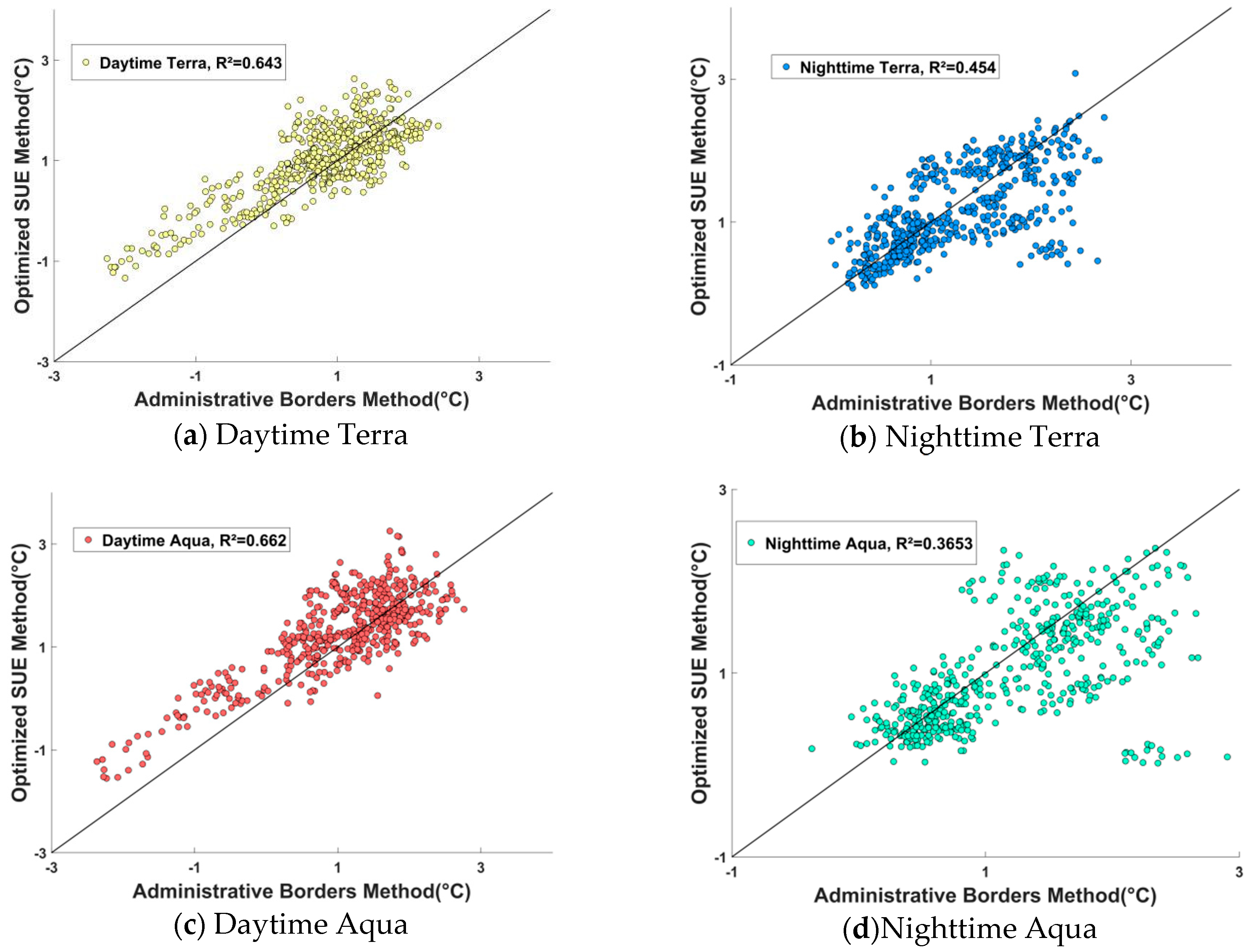
3.3. Predictive Models of SUHIs

We developed predictive models for the SUHI obtained from the AB and OSUE methods during the daytime and nighttime. The models based on the combination of the natural and social factors accounted for 31.8–74.3% of the SUHIs (Table S1). The natural condition factors included the Pr, M index, and NDVI. The social factors included the GDP, population and RN. The NDVI had negative effects on the daytime SUHI in both the AB and OSUE methods, while the RN had a positive influence. The NDVI and Pr had positive effects on the nighttime SUHI with both the AB and OSUE methods, while M had a negative influence. The remaining factors had opposite effects on the SUHI based on the two methods.

The relative contributions of the potential drivers can be quantified by the standard coefficients of the regression models (Figure 11). The explanation rates of natural conditions for the SUHIs with the AB method were 50.9% (daytime Terra), 54.4% (daytime Aqua), 42.1% (nighttime Terra), and 47% (nighttime Aqua). The explanation rates of social development for the SUHIs with the AB method were 22.1% (daytime Terra), 19.9% (daytime Aqua), 12.3% (nighttime Terra), and 11.6% (nighttime Aqua). The explanation rates of natural conditions for the SUHIs with the OSUE method were 60% (daytime Terra), 53.5% (daytime Aqua), 26.6% (nighttime Terra), and 34.7% (nighttime Aqua). The explanation rates of social development for the SUHIs with the OSUE method were 5.1% (daytime Terra), 8.9% (daytime Aqua), 5.2% (nighttime Terra), and 5.8% (nighttime Aqua). The results showed that vegetation had a significant impact as a temperature regulator of the daytime SUHI, whether with the AB method or the OSUE method. The daytime SUHI calculated with the AB method was significantly more affected by the social development factors than that calculated by the OSUE method. In the AB method, RN is an important factor, which means that the proportion of urban and rural pixels participating in the calculation of the SUHI would have a relatively large impact on the results.

4. Discussion

Although the SUHI intensity is primarily controlled by diverse rural extents, the methods for selecting appropriate rural extents for future research remain largely unclear. Few previous studies on the uncertainty of SUHI intensity have focused on the differences in the driving factors of the calculations from different methods, with most of the comparison generally focusing on the spatiotemporal distribution [27,46]. However, the most important purpose of UHI research is to explore the drivers of the UHI phenomenon and to propose further mitigation suggestions. Therefore, in this study, we not only compared the differences between the AB and OSUE methods from the perspective of the spatiotemporal patterns but also analyzed the differences in the driving factors.

In Section 3, the differences between the two methods were fully demonstrated. We can clearly see that, in most cases, the two methods exhibited similar temporal and spatial patterns, especially on the national scale (Figure 3 and Figure 4) and the monthly scale (Figure 8 and Figure 9). Specifically, the daytime in the southeastern areas and the nighttime in the northern areas had higher SUHI intensities than the rest of China, which was consistent with previous conclusions on the SUHI in China in the literature [21]. From the perspective of the driving factors, both methods showed a very large daily difference due to the different driving factors of UHI during the daytime and nighttime, which were mentioned in several previous studies [21,32,47,48]. A comparison of the above two points, with the conclusions of previous studies, shows that the FB and CD or SUA showed differences in SUHI intensity, although the differences in the spatiotemporal modes were negligible. The two methods showed great differences in terms of anthropogenic factors. The most likely reason for these differences was that the spatial extents (administrative borders) of the data used in the AB method for the driving factor analysis were more closely aligned with the true borders.

On this basis, we conducted a thought experiment from the perspective of the standardization of the calculation of the SUHI, that of, is the AB method a valuable option for the calculation of SUHI intensity in multiple cities? Although some researchers argue that it is not appropriate [38], the AB method is simple and versatile. Moreover, two additional reasons support our use of the AB method in the SUHI intensity calculations: (i) for Chinese cities, the rural areas within the administrative borders typically correspond well to the associated size of the urban areas [27] (ii) and some studies have confirmed that the administrative division has a significant impact on the spatial form of an urban area [49]. The above two points support the rationality of using the AB method to calculate the SUHI intensity. According to the above points, we have sufficient evidence that the AB method has great application potential for future UHI studies, especially in regard to the analysis of the anthropogenic driving factors.

The strength of the UHI effect is generally measured based on the SUHI intensity, and this method can be used in most cities in China or other parts of the world. Furthermore, both the AB method and the OSUE method used in this paper have their own advantages; thus, these two methods can be applied for research around the world. We need to point out that each city has its own unique characteristics, including but not limited to the climate, development mode, urban form and urban planning. Our conclusions based on a spatial-temporal analysis may not be universally suitable to all regions or time spans. However, the conclusions obtained here by evaluating the potential of the AB method in the analysis of SUHI driving factors provide a valuable reference for future research.

It is important to note that several factors should be investigated in future studies. The first is the uncertainty created by the remote sensing data. Although the accuracy of the MODIS products has been demonstrated in many studies, obtaining more reliable temperature data is an important direction for urban heat island research. The second factor is the exploration of other driving factors. It has been reported that air pollution [48] and energy consumption [17,50] will lead to an increase in urban heat islands, but the factors that have been identified thus far cannot fully explain the occurrence of urban heat islands. Future research on the factors that influence the UHI and are closely related to urban development is of great significance. The third point is the exploration of the calculation methods for urban heat island intensity. There is still no unified calculation standard for the SUHI intensity, which is an important direction that can be explored in the future.

5. Conclusions

By comparing the differences between the two methods of AB and OSUE, we not only mapped the spatiotemporal patterns in 36 major cities in mainland China, but also explored whether administrative borders represent an appropriate standard range for the rural extent in SUHI intensity calculations. The SUHI intensity obtained from the two methods did not show significantly different spatial distributions or temporal trends, especially seasonally. The daytime in the southeastern areas and the nighttime in the northern areas had higher SUHI intensities than the rest of China and the daytime SUHI intensity is the highest in summer and the lowest in winter. However, in the regression analysis with the driving factors, the anthropogenic factors had a more significant influence on the SUHI intensity of the AB method. In the AB method, GDP and population were two of the most important drivers of SUHI intensity during the day and night, respectively. These conclusions stress the necessity of further research of the UHI drivers. We suggest that in future studies on the socioeconomic drivers of UHIs such as the analysis of negative spillover effect from UHIs by using a spatial econometrics model, more attention should be paid to the application of the AB method. However, uncertainties remain in the current study and the standardized calculation for SUHI intensity needs deeper research through attribution analysis or numeric modeling.

As administrative divisions are a universal phenomenon in human society, the conclusions of this study also have a certain reference value at the global scale and are worthy of further expansion such as adding more ponderable drivers in future research.

References

- Nations, U. World urbanization prospects: The 2014 revision, highlights. In Department of Economic and Social Affairs; United Nations: New York, NY, USA, 2014. [Google Scholar]
- DeFries, R. Terrestrial Vegetation in the Coupled Human-Earth System: Contributions of Remote Sensing. Annu. Rev. Environ. Resour. 2008, 33, 369–390. [Google Scholar] [CrossRef]
- Grimm, N.B.; Faeth, S.H.; Golubiewski, N.E.; Redman, C.L.; Wu, J.G.; Bai, X.M.; Briggs, J.M. Global change and the ecology of cities. Science 2008, 319, 756–760. [Google Scholar] [CrossRef]
- Howard, L. Climate of London deduced from meteorological observation. Harvey Darton 1833, 1, 1–24. [Google Scholar]
- Reid, W.V. Biodiversity hotspots. Trends Ecol. Evol. 1998, 13, 275–280. [Google Scholar] [CrossRef]
- Chen, X.L.; Zhao, H.M.; Li, P.X.; Yin, Z.Y. Remote sensing image-based analysis of the relationship between urban heat island and land use/cover changes. Remote Sens. Environ. 2006, 104, 133–146. [Google Scholar] [CrossRef]
- Li, H.D.; Meier, F.; Lee, X.H.; Chakraborty, T.; Liu, J.F.; Schaap, M.; Sodoudi, S. Interaction between urban heat island and urban pollution island during summer in Berlin. Sci. Total Environ. 2018, 636, 818–828. [Google Scholar] [CrossRef] [PubMed]
- Arnfield, A.J. Two decades of urban climate research: A review of turbulence, exchanges of energy and water, and the urban heat island. Int. J. Climatol. 2003, 23, 1–26. [Google Scholar] [CrossRef]
- Bernstein, L.; Bosch, P.; Canziani, O.; Chen, Z.; Christ, R.; Riahi, K. IPCC, 2007: Climate Change 2007: Synthesis Report; IPCC: Geneva, Switzerland, 2008. [Google Scholar]
- Patz, J.A.; Campbell-Lendrum, D.; Holloway, T.; Foley, J.A. Impact of regional climate change on human health. Nature 2005, 438, 310–317. [Google Scholar] [CrossRef]
- Lafortezza, R.; Carrus, G.; Sanesi, G.; Davies, C. Benefits and well-being perceived by people visiting green spaces in periods of heat stress. Urban For. Urban Green. 2009, 8, 97–108. [Google Scholar] [CrossRef]
- Gong, P.; Liang, S.; Carlton, E.J.; Jiang, Q.W.; Wu, J.Y.; Wang, L.; Remais, J.V. Urbanisation and health in China. Lancet 2012, 379, 843–852. [Google Scholar] [CrossRef]
- Li, K.N.; Chen, Y.H.; Wang, M.J.; Gong, A. Spatial-temporal variations of surface urban heat island intensity induced by different definitions of rural extents in China. Sci. Total Environ. 2019, 669, 229–247. [Google Scholar] [CrossRef]
- Rao, P.K. Remote Sensing of Urban Heat Islands from an Environmental Satellite. Bull. Am. Meteorol. Soc. 1972, 53, 647–648. [Google Scholar]
- Roth, M.; Oke, T.; Emery, W. Satellite-derived urban heat islands from three coastal cities and the utilization of such data in urban climatology. Int. J. Remote Sens. 1989, 10, 1699–1720. [Google Scholar] [CrossRef]
- Gallo, K.P.; Tarpley, J.D.; McNab, A.L.; Karl, T.R. Assessment of urban heat islands: A satellite perspective. Atmos. Res. 1995, 37, 37–43. [Google Scholar] [CrossRef]
- Imhoff, M.L.; Zhang, P.; Wolfe, R.E.; Bounoua, L. Remote sensing of the urban heat island effect across biomes in the continental USA. Remote Sens. Environ. 2010, 114, 504–513. [Google Scholar] [CrossRef]
- Peng, S.; Piao, S.; Ciais, P.; Friedlingstein, P.; Ottle, C.; Breon, F.M.; Nan, H.; Zhou, L.; Myneni, R.B. Surface urban heat island across 419 global big cities. Environ. Sci. Technol. 2012, 46, 696–703. [Google Scholar] [CrossRef]
- Clinton, N.; Gong, P. MODIS detected surface urban heat islands and sinks: Global locations and controls. Remote Sens. Environ. 2013, 134, 294–304. [Google Scholar] [CrossRef]
- Zhang, P.; Imhoff, M.L.; Wolfe, R.E.; Bounoua, L. Characterizing urban heat islands of global settlements using MODIS and nighttime lights products. Can. J. Remote Sens. 2010, 36, 185–196. [Google Scholar] [CrossRef]
- Zhou, D.; Zhao, S.; Liu, S.; Zhang, L.; Zhu, C. Surface urban heat island in China’s 32 major cities: Spatial patterns and drivers. Remote Sens. Environ. 2014, 152, 51–61. [Google Scholar] [CrossRef]
- Zhou, D.; Bonafoni, S.; Zhang, L.; Wang, R. Remote sensing of the urban heat island effect in a highly populated urban agglomeration area in East China. Sci. Total Environ. 2018, 628, 415–429. [Google Scholar] [CrossRef]
- Voogt, J.A.; Oke, T.R. Thermal remote sensing of urban climates. Remote Sens. Environ. 2003, 86, 370–384. [Google Scholar] [CrossRef]
- Lai, J.; Zhan, W.; Huang, F.; Quan, J.; Hu, L.; Gao, L.; Ju, W. Does quality control matter? Surface urban heat island intensity variations estimated by satellite-derived land surface temperature products. ISPRS J. Photogramm. Remote Sens. 2018, 139, 212–227. [Google Scholar] [CrossRef]
- Chakraborty, T.; Lee, X. A simplified urban-extent algorithm to characterize surface urban heat islands on a global scale and examine vegetation control on their spatiotemporal variability. Int. J. Appl. Earth Obs. Geoinf. 2019, 74, 269–280. [Google Scholar] [CrossRef]
- Yao, R.; Wang, L.C.; Huang, X.; Chen, J.P.; Li, J.R.; Niu, Z.G. Less sensitive of urban surface to climate variability than rural in Northern China. Sci. Total Environ. 2018, 628, 650–660. [Google Scholar] [CrossRef]
- Lai, J.; Zhan, W.; Huang, F.; Voogt, J.; Bechtel, B.; Allen, M.; Peng, S.; Hong, F.; Liu, Y.; Du, P. Identification of typical diurnal patterns for clear-sky climatology of surface urban heat islands. Remote Sens. Environ. 2018, 217, 203–220. [Google Scholar] [CrossRef]
- Yao, R.; Wang, L.C.; Huang, X.; Niu, Z.G.; Liu, F.F.; Wang, Q. Temporal trends of surface urban heat islands and associated determinants in major Chinese cities. Sci. Total Environ. 2017, 609, 742–754. [Google Scholar] [CrossRef]
- Zhang, X.Y.; Friedl, M.A.; Schaaf, C.B.; Strahler, A.H.; Schneider, A. The footprint of urban climates on vegetation phenology. Geophys. Res. Lett. 2004, 31. [Google Scholar] [CrossRef]
- Li, X.M.; Zhou, Y.Y.; Asrar, G.R.; Imhoff, M.; Li, X.C. The surface urban heat island response to urban expansion: A panel analysis for the conterminous United States. Sci. Total Environ. 2017, 605, 426–435. [Google Scholar] [CrossRef]
- Quan, J.L.; Zhan, W.F.; Chen, Y.H.; Wang, M.J.; Wang, J.F. Time series decomposition of remotely sensed land surface temperature and investigation of trends and seasonal variations in surface urban heat islands. J. Geophys. Res. Atmos. 2016, 121, 2638–2657. [Google Scholar] [CrossRef]
- Zhou, D.C.; Zhao, S.Q.; Zhang, L.X.; Sun, G.; Liu, Y.Q. The footprint of urban heat island effect in China. Sci. Rep. 2015, 5, 11160. [Google Scholar] [CrossRef]
- Meng, Q.Y.; Zhang, L.L.; Sun, Z.H.; Meng, F.; Wang, L.; Sun, Y.X. Characterizing spatial and temporal trends of surface urban heat island effect in an urban main built-up area: A 12-year case study in Beijing, China. Remote Sens. Environ. 2018, 204, 826–837. [Google Scholar] [CrossRef]
- Zhou, D.; Zhao, S.; Zhang, L.; Liu, S. Remotely sensed assessment of urbanization effects on vegetation phenology in China’s 32 major cities. Remote Sens. Environ. 2016, 176, 272–281. [Google Scholar] [CrossRef]
- Schwarz, N.; Lautenbach, S.; Seppelt, R. Exploring indicators for quantifying surface urban heat islands of European cities with MODIS land surface temperatures. Remote Sens. Environ. 2011, 115, 3175–3186. [Google Scholar] [CrossRef]
- Zhou, D.C.; Xiao, J.F.; Bonafoni, S.; Berger, C.; Deilami, K.; Zhou, Y.Y.; Frolking, S.; Yao, R.; Qiao, Z.; Sobrino, J.A. Satellite Remote Sensing of Surface Urban Heat Islands: Progress, Challenges, and Perspectives. Remote Sens. 2019, 11, 48. [Google Scholar] [CrossRef]
- Cui, Y.; Xu, X.; Dong, J.; Qin, Y. Influence of Urbanization Factors on Surface Urban Heat Island Intensity: A Comparison of Countries at Different Developmental Phases. Sustainability 2016, 8, 706. [Google Scholar] [CrossRef]
- Sun, R.H.; Lu, Y.H.; Yang, X.J.; Chen, L.D. Understanding the variability of urban heat islands from local background climate and urbanization. J. Clean. Prod. 2019, 208, 743–752. [Google Scholar] [CrossRef]
- Wan, Z.M.; Dozier, J. A generalized split-window algorithm for retrieving land-surface temperature from space. IEEE Trans. Geosci. Remote Sens. 1996, 34, 892–905. [Google Scholar]
- Wan, Z.M. New refinements and validation of the MODIS Land-Surface Temperature/Emissivity products. Remote Sens. Environ. 2008, 112, 59–74. [Google Scholar] [CrossRef]
- Wan, Z.M. New refinements and validation of the collection-6 MODIS land-surface temperature/emissivity product. Remote Sens. Environ. 2014, 140, 36–45. [Google Scholar] [CrossRef]
- Li, X.C.; Zhang, Y.J.; Jin, X.L.; He, Q.N.; Zhang, X.P. Comparison of digital elevation models and relevant derived attributes. J. Appl. Remote Sens. 2017, 11, 046027. [Google Scholar] [CrossRef]
- Schneider, A.; Friedl, M.A.; Potere, D. A new map of global urban extent from MODIS satellite data. Environ. Res. Lett. 2009, 4, 044003. [Google Scholar] [CrossRef]
- Schneider, A.; Friedl, M.A.; Potere, D. Mapping global urban areas using MODIS 500-m data: New methods and datasets based on ‘urban ecoregions’. Remote Sens. Environ. 2010, 114, 1733–1746. [Google Scholar] [CrossRef]
- Dobson, J.E.; Bright, E.A.; Coleman, P.R.; Durfee, R.C.; Worley, B.A. LandScan: A global population database for estimating populations at risk. Photogramm. Eng. Remote Sens. 2000, 66, 849–857. [Google Scholar]
- Yao, R.; Wang, L.; Huang, X.; Niu, Y.; Chen, Y.; Niu, Z. The influence of different data and method on estimating the surface urban heat island intensity. Ecol. Indic. 2018, 89, 45–55. [Google Scholar] [CrossRef]
- Yao, R.; Wang, L.; Huang, X.; Zhang, W.; Li, J.; Niu, Z. Interannual variations in surface urban heat island intensity and associated drivers in China. J. Environ. Manag. 2018, 222, 86–94. [Google Scholar] [CrossRef]
- Cao, C.; Lee, X.; Liu, S.; Schultz, N.; Xiao, W.; Zhang, M.; Zhao, L. Urban heat islands in China enhanced by haze pollution. Nat. Commun. 2016, 7, 12509. [Google Scholar] [CrossRef]
- Gao, X.; Long, C.X. Cultural border, administrative border, and regional economic development: Evidence from Chinese cities. China Econ. Rev. 2014, 31, 247–264. [Google Scholar] [CrossRef]
- McCarthy, M.P.; Best, M.J.; Betts, R.A. Climate change in cities due to global warming and urban effects. Geophys. Res. Lett. 2010, 37. [Google Scholar] [CrossRef]
© 2020 by the authors. Licensee MDPI, Basel, Switzerland. This article is an open access article distributed under the terms and conditions of the Creative Commons Attribution (CC BY) license (http://creativecommons.org/licenses/by/4.0/).
Share and Cite
Niu, L.; Tang, R.; Jiang, Y.; Zhou, X. Spatiotemporal Patterns and Drivers of the Surface Urban Heat Island in 36 Major Cities in China: A Comparison of Two Different Methods for Delineating Rural Areas. Sustainability 2020, 12, 478. https://doi.org/10.3390/su12020478
Niu L, Tang R, Jiang Y, Zhou X. Spatiotemporal Patterns and Drivers of the Surface Urban Heat Island in 36 Major Cities in China: A Comparison of Two Different Methods for Delineating Rural Areas. Sustainability. 2020; 12(2):478. https://doi.org/10.3390/su12020478
Chicago/Turabian StyleNiu, Lu, Ronglin Tang, Yazhen Jiang, and Xiaoming Zhou. 2020. "Spatiotemporal Patterns and Drivers of the Surface Urban Heat Island in 36 Major Cities in China: A Comparison of Two Different Methods for Delineating Rural Areas" Sustainability 12, no. 2: 478. https://doi.org/10.3390/su12020478
APA StyleNiu, L., Tang, R., Jiang, Y., & Zhou, X. (2020). Spatiotemporal Patterns and Drivers of the Surface Urban Heat Island in 36 Major Cities in China: A Comparison of Two Different Methods for Delineating Rural Areas. Sustainability, 12(2), 478. https://doi.org/10.3390/su12020478