Multi-Objective Intelligent Optimization of Superheated Steam Temperature Control Based on Cascaded Disturbance Observer

Abstract

Superheated steam temperature (SST) is one of the most critical parameters for the process safety, overall efficiency and pollution reduction of coal-fired power plants. However, SST control is challenging due to various disturbances and model uncertainties, especially in the face of the growing penetration of intermittent renewable energy into the power grid. To this end, a cascaded Disturbance Observer-PI (DOB-PI) control strategy is proposed to enhance control performance. The observer design and parameter tuning are carried out through mechanism analysis on the proposed structure. Furthermore, a robust loop shaping method is introduced as a hard constraint to balance the control performance and robustness. The controller parameters are optimized based on the multi-objective artificial bee colony optimization (MOABC) algorithm. Simulation results show that the proposed cascaded DOB-PI control strategy can significantly improve the disturbance rejection performance of both the inner- and outer-loops of the SST control system. This paper indicates promising prospects for the proposed method in future applications.

1. Introduction

As a key parameter in the operation of power plant boilers, superheated steam temperature (SST) is of great significance to the economic and safe operation of the unit. On the one hand, a superheated steam temperature that is beyond safe range will have an adverse impact on the unit. On the other, steam with a lower superheated steam temperature will reduce the efficiency of the whole plant and bring about safety problems such as carrying water in the last stage of the turbine, which may damage the last stage blades. A superheated steam temperature higher than the set-point level will cause unrecoverable damage to the steam tube, regardless of whether the overtemperature was long-term or short-term [1,2], even causing the unit to shut down. Therefore, the superheated temperature needs to be adjusted within a limited operating range. It is generally recommended that the fluctuation range of superheated steam temperature is ±5 °C from its set-point [3,4]. On the other hand, even if the above conditions are met, frequent temperature variation will still produce thermal stress, resulting in metal failure.

With the continuous development and large-scale grid connection of renewable energy, such as solar and wind power generation, new challenges to the control of superheated steam temperature in power plants emerge [5,6]. It is estimated that renewable energy will increase by 2.8% per year and account for 1/4 of global electricity generation around 2040 [7]. The randomness and intermittency of renewable energy result in great challenges to the stability and reliability of the power grid [8]. One of the mature feasible measures is to improve the tracking ability of thermal power units to the instructions of automatic generation control (AGC), so as to stabilize the load deviation in real time [9]. Generally speaking, a wide range of power regulation corresponds to a large deviation of the SST from its set-point [10]. In other words, the load flexibility that can be achieved by the power plant depends to a large extent on the control performance of the superheated steam temperature loop [11]. A strong SST control loop will enable the power plant to participate in a wider-range of load regulation, allowing more renewable energy to be connected to the grid.

Since SST is a typical thermal process with large inertia and is affected by various disturbances, the cascaded control structure is usually adopted. Compared with the single loop control structure, the secondary controller can observe in advance and quickly attenuate the disturbance of the inner-loop, thus significantly improving the performance of the system. However, when working conditions change greatly, the conventional cascaded PI control of SST is limited by the PI controller and cannot achieve satisfactory control performance [12]. Due to the large lag characteristic of the outer-loop object, the disturbance rejection ability of the outer-loop needs to be strengthened. For these reasons, many improved and advanced control strategies have been proposed to improve the control effect of SST, such as fractional order PID control [13], fuzzy control [14], internal mode control (IMC) [15], fuzzy model predictive controller (MPC) [16], neuro-fuzzy generalized predictive control (GPC) [17]. However, these control strategies are seldom applied in actual process control for the following reasons:

(1). Some control strategies require the accurate mathematical model of SST to design the controller, while the model uncertainty of the actual object exists objectively and varies with time and working conditions.

(2). Due to the complexities in computation, most of the advanced control strategies are hard to implement on the traditional distributed control system (DCS), while the external computer has some security problems such as communication interruption.

DOB was proposed by Ohnishi et al. [18] in the early 1980s and is considered to be an effective method of disturbance rejection [19]. Its fundamental idea is to bring together external disturbance and model uncertainty as a lumped disturbance, and then estimate and eliminate the disturbance through a reasonably designed disturbance observer [20]. The core of the disturbance observer based control (DOBC) is the design of the low-pass filter, which suppresses disturbance in low- and medium-frequency ranges and removes the influence of high-frequency measurement noise. With the advancing of research, the DOB has been extended to time-delay, non-minimum phase and nonlinear systems [19,21,22]. The DOB has been utilized in many practical controls [23,24,25,26], due to its powerful aptitude for disturbance rejection and uncertainty compensation. As well as this, the traditional frequency-domain DOB only needs output and input information to observe disturbances, which is engineering-friendly.

However, most of the current DOBC applications are single-loop structures. This paper will develop a cascaded DOB-PI control scheme based on analysis of a cascaded DOB system. The disturbance of the inner- and outer-loop will be estimated and mainly suppressed by the cascaded DOB system, thus significantly improving the control performance of the system. There is a tradeoff problem in the outer-loop filter design of the cascaded DOB system, which is different from that of the single-loop DOB and will be solved through a robust loop shaping design method. In order to obtain better control performance and system robustness at the same time, the inner- and outer-loop PI controllers are optimized by the Pareto-based multi-objective artificial bee colony algorithm (MOABC), which has been widely used in different fields [27,28,29,30]. Compared with other intelligent algorithms, it has the advantages of less preset parameters, a concise and clear structure and is convenient for implementation and application. The combination of a stability region and an intelligent optimization algorithm can optimize the controller parameters and ensure system stability simultaneously [11,31].

The main innovations of this study are summarized as follows:

(a)

A cascaded DOB-PI control strategy based on traditional control system is proposed to improve the performance of the control system.

(b)

A multi-objective optimization model of the inner- and outer-loop PI controller is established to deal with conflicting objectives and reduce the conservatism of the control, based on the design of a cascaded DOB system.

(c)

The optimized Pareto front and simulation show the overwhelming advantages of the proposed cascaded DOB-PI control strategy, which significantly improves the disturbance rejection performance of the inner and outer-loop.

The rest of the paper is arranged as follows. Section 2 briefly introduces the SST model and control objectives. The proposed cascaded DOB-PI control system and its parameter design are introduced in Section 3, based on analysis of the cascaded DOB system. In Section 4, the parameters of the observer and controller of the cascaded DOB-PI system are optimized, and the significant improvement in control performance is illustrated by simulations. Section 5 shows the comparison with cascaded PI control strategy and the simulation of model mismatch, in order to verify the superiority and robustness of the control strategy. Conclusions are drawn in the last section.

2. System Description

2.1. The Model Description of SST

In this paper, the power plant superheater in [11] is taken into account. Figure 1 shows the flowchart of the power plant superheater. In this control structure, the flow of cooling water is regulated by controlling the valve position, so as to control the steam temperature at the outlet of the 1st stage superheater. The cooling water comes from an intermediate stage of the boiler feed water pump.

Figure 2 shows the structure diagram of a simplified cascaded SST control system, in which the distributed parameter superheating system is approximated to two linear transfer function models $G_1(s)$ and $G_2(s)$.

In this control system, the control variable is the opening of the spray valve, denoted as $u_1$. $y_1$ is the inner-loop output, which represents steam temperature downstream of the desuperheater. It can quickly reflect the influence of the change in spray water on the steam temperature and is beneficial to the disturbance suppression of the inner-loop. The set-point $u_2$ of the inner-loop controller $G_{C1}(s)$ is given by the output of the main controller $G_{C2}(s)$. The output of the outer-loop $y_2$ is the primary steam temperature. $r$ is the primary steam temperature set-point, which is generally a constant. In practical application, a PI controller is selected for both inner and outer-loop controllers.

The most common disturbances in the inner-loop are changes in feed water temperature and pressure, which can lead to temperature fluctuations at a certain valve opening. They are approximately modelled as a step-type disturbance $d_1$.

The outer-loop disturbances, such as load regulation, combustion instability and coal quality change, influence the primary steam temperature mainly through the 2nd stage superheater, which are modelled as a step-type disturbance $d_2$.

Based on the open-loop experimental data, the following inner- and outer-loop object models are obtained [11],

$$\begin{array}{l}{G}_1(\mathrm{s})=\frac{y_1}{u_1}=-\frac{1}{{(1+9s)}^4}\\ G_2(\mathrm{s})=\frac{y_2}{y_1}=\frac{1.5}{{(1+60s)}^2}\end{array}$$

(1)

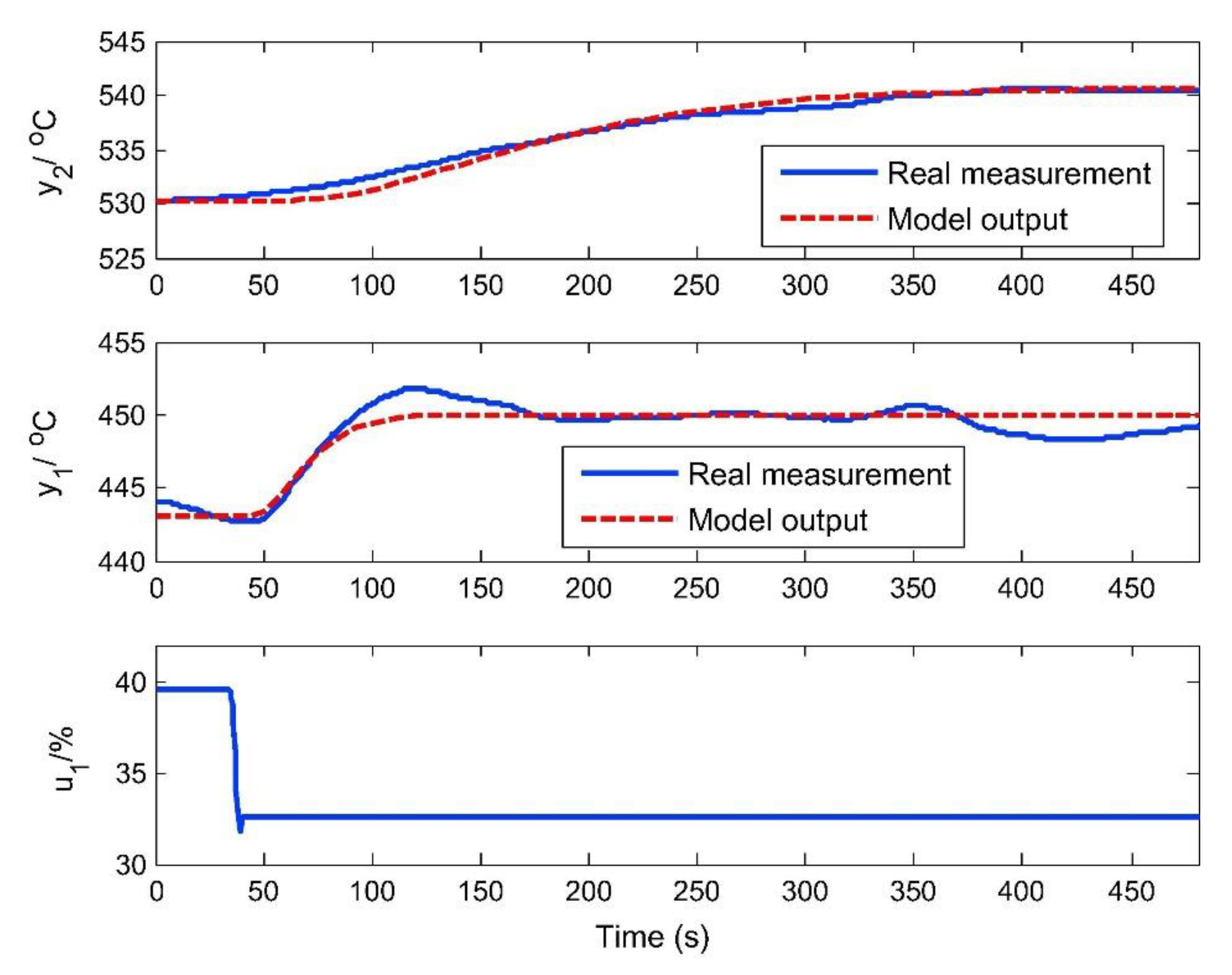
The comparison between experimental measurements and model outputs are shown in Figure 3. It can be considered that the identification model can well reflect the dynamic characteristics of SST. By comparison, it can also be seen that the inner-loop dynamic is significantly faster than the outer-loop.

It should be noted that the following control difficulties were faced in the actual operation:

• The influence of multiple disturbances makes the control parameters of the inner- and outer-loop deviate from target value.
• High order and large lag dynamics of the superheater lead to slow responses to the disturbances.
• Due to the high complexity and nonlinearity of the SST system, it is difficult to obtain an accurate mathematical model. The transfer function varies with time and operating conditions, so the control system is required to be robust enough withstand modelling uncertainties.

In this paper, DOB is regarded as a control system patch, that is, the controller and the observer can be designed separately. Further, the parameters of the inner- and outer-loop controllers are optimized separately for the following two considerations:

(a) The inner-loop dynamics are significantly faster than the outer-loop. The main and auxiliary loop controllers can be designed separately;

(b) The main disturbance channels of the inner- and outer-loop are different. The inner-loop disturbance mainly acts on the pressure-flow channel, while the outer-loop disturbance is in the enthalpy-temperature channel.

2.2. Control Objectives

This section describes the control objectives of the SST cascaded control system and some index functions to evaluate control performance or robustness.

For the inner-loop, both disturbance rejection and set-point tracking capabilities need to be considered. At the same time, the control system needs to be robust enough to deal with model uncertainties.

For the outer-loop, the primary task is to restrain the influence of disturbance and ensure the robustness of the control system against model uncertainties. The ability to track reference is weakened because the SST set-point is generally constant.

The integrated absolute error (IAE) index reflects the integral error between the control output and the reference. It is used as an evaluation index of control performance.

$$IAE={\displaystyle {\int }_0^{\infty }\left|r(t)-y(t)\right|}dt$$

(2)

where $r(t)$ is the reference, and $y(t)$ is the controlled output in response to the set-point tracking or disturbance rejection. In practical application, the integration time is set large enough to make the output track the set-point completely.

The robustness index used in this paper is the maximum sensitivity function, defined as:

$$M_S=\underset{\omega }{\max }\left|\frac{1}{1+L(j\omega )}\right|$$

(3)

where $L(s)$ is the open-loop transfer function of the control system. The robustness index $M_S$ physically represents how significantly the closed-loop control system will vary in the presence of open-loop modelling perturbation [32]. Considering traditional frequency domain analysis, the $M_S$ index represents the reciprocal of the distance between the frequency response curve of the open-loop transfer function and the point (−1, j0). The smaller the $M_S$ index is, the farther the distance from the critical point, and the better the robustness.

In this paper, the disturbance rejection performance and the robustness to model uncertainty of the inner- and outer-loops will be improved by the cascaded DOB system. The above tradeoff problems for disturbance rejection, set-point tracking and robustness will be solved via multi-objective optimization.

3. Analysis of Cascaded DOB-PI System

The cascaded DOB-PI control strategy is proposed in this section, based on analysis of the cascaded DOB control structure.

3.1. Cascaded Disturbance Observer

As shown in Figure 4, the cascaded DOB control structure is mentioned firstly in [33], and it is a natural extension of the traditional single-loop DOB.

The inner-loop of the cascaded DOB structure is the traditional single-loop DOB, which is the basis of the cascaded DOB.

Figure 5 shows the general structure of a disturbance observer for a Single-input and single-output (SISO) plant. There are three inputs to the system, namely, command input, disturbance and sensor noise, denoted as $c_1$, $d_1$ and ${\zeta }_1$, respectively. $u_1$ is the control input, which will act on the physical plant and be sent to DOB for disturbance observation. $G_1(s)$ represents the actual controlled plant, while $G_{1n}(s)$ is the nominal plant model. DOB observes the lumped disturbance of external disturbance and model mismatch, and feeds back the disturbance estimation ${\widehat{d}}_1$ to eliminate disturbance. $Q_1(s)$ is a low-pass filter with unity gain that needs to be designed.

For the single loop DOB, the transfer function from each input to output $y_1$ is

$$y_1=G_{yc}(s)\cdot c_1+G_{yd}(s)\cdot d_1+G_{y\xi }(s)\cdot {\xi }_1,$$

(4)

where (for simplicity, the ‘s’ in the right formula is omitted):

$$G_{yc}(s)=\frac{G_1\cdot G_{1n}}{G_{1n}-Q_1{G}_{1n}+Q_1{G}_1},$$

(5)

$$G_{yd}(s)=\frac{G_1\cdot G_{1n}(1-Q_1)}{G_{1n}-Q_1{G}_{1n}+Q_1{G}_1},$$

(6)

$$G_{y\xi }(s)=\frac{G_1\cdot Q_1}{G_{1n}-Q_1{G}_{1n}+Q_1{G}_1}.$$

(7)

If the filter $Q_1(s)$ is selected as a low-pass form, that is, $\underset{s\to 0}{\lim }{Q}_1(s)=1$, then (4) becomes $y_1=G_{1n}(s)\cdot c_1+{\xi }_1$. This indicates that DOB rejects the lumped disturbance and restores the plant to the nominal state in the low-frequency domain.

Based on Mayson’s rule, the following closed-loop transfer functions can be obtained:

$$D_1(s)=\frac{{\widehat{d}}_1}{d_1}=\frac{G_1{Q}_1{G}_{1n}^{-1}}{1-Q_1+Q_1{G}_1{G}_{1n}^{-1}}=\frac{G_1{Q}_1}{G_{1n}-Q_1{G}_{1n}+Q_1{G}_1}.$$

(8)

Since $Q_1(s)$ is of unity gain, the DOB can provide an accurate estimation of the real disturbance. On the other hand, the sensor noise is generally considered to be high frequency, at this time $Q_1(s)\approx 0$, so (4) becomes $y_1=G_1(s)\cdot c_1+G_1(s)\cdot d_1$. The disturbance observer loop is basically inactive, and the output is not affected by high frequency sensor noise.

The abilities of the inner-loop DOB are introduced above, then the outer-loop DOB is analyzed.

As can be seen from Figure 4, the working principle of the outer-loop DOB is basically the same as that of the inner-loop. When the inner-loop plant is recovered as the nominal model, it is the equivalent of adding a unit gain low-pass filter $Q_3(s)$ to the feedback channel.

It should be noted that the design of the outer-loop filter $Q_2(s),Q_3(s)$ needs to consider not only the performance of the disturbance observation but also the effect on the inner-loop. Since the cancellation signal of the outer-loop is fed back into the front of the inner-loop, the set-point of the inner-loop will be changed, thus affecting the inner-loop output. In the SST control system, the allowable fluctuation ranges of the 1st stage superheated steam temperature and valve opening are limited, so the outer-loop cannot blindly pursue the performance of disturbance rejection. This problem will be considered in the filter design.

3.2. Cascaded DOB-PI Control System

By applying the above cascaded DOB to the traditional cascaded SST control system, the following control system can be obtained (Figure 6).

It is a natural combination of these two systems, and will not change the original cascaded control system structure, where $G_{e1}(s)$ is the equivalent transfer function of the inner-loop.

$$G_{e1}(s)=\frac{G_{C1}{G}_1}{1+G_{C1}{G}_1}$$

(9)

Therefore, the outer-loop DOB is here consistent with that in 3.1. It should be especially pointed out that, compared with the outer-loop, the dynamic of the inner-loop is very fast, so it has less influence on the outer-loop. In contrast to the traditional cascaded control system, the set-point of the inner-loop is given by the output of the main controller and the outer-loop DOB. During the action of disturbance $d_2$, the outer-loop DOB can quickly estimate and feedback disturbance (change the set-point of the inner-loop). So, the SST fluctuation caused by this disturbance can be quickly stabilized by adjusting the opening of the spray valve. As for inner-loop disturbance $d_1$, the disturbance is estimated and fed back directly through the inner-loop DOB, and then suppressed by adjusting the opening of the spray valve. This is the key advantage of the cascaded DOB-PI control system compared with traditional cascaded control systems. This point of view will be verified by subsequent simulations. In the cascaded DOB-PI control system, the Q filters and inner- and outer-loop controller parameters need to be further designed.

The stability of the control system needs special consideration. In this paper, the controller parameter stability region drawing method in [11] is adopted and used as the initialization region for multi-objective optimization.

Based on the Nyquist stability criterion, for an open-loop stable plant $G(s)$, the control system is stable if and only if the Nyquist plot of $G_C(s)G(s)$ does not encircle the critical point (−1, j0). Then, equations including $k_p,k_i$ and $\omega$ can be obtained by

$$G_C(j\omega )G(j\omega )=-1,$$

(10)

where $G_C(j\omega )$ and $G(j\omega )$ are the transfer functions of the controller and the controlled object, respectively. That is, let the real and imaginary part of $G_C(j\omega )G(j\omega )+1$ are equal to 0 respectively. By gradually increasing the value of $\omega$ from 0, the corresponding stable region of the controller parameters can be obtained by numerical method. The stable region will be used as the search area for controller optimization.

4. Design and Simulation

In this section, firstly, the low-pass filters for the cascaded DOB system are designed. Then, the parameters of the inner and outer-loop PI controllers are introduced in Section 3.2 and optimized using the multi-objective optimization algorithm. In the cascaded DOB simulation in Section 4.2, no feedback controller is introduced (the control structure is detailed in Figure 4). The controller simulations in Section 4.3 and Section 4.4 are based on the designed cascaded DOB system (i.e., the control structure in Figure 6). In this section simulation, the actual model is taken as the nominal model.

4.1. Multi-Objective Artificial Bee Colony Optimization

In this section, the principles of MOABC are briefly introduced.

Artificial Bee Colony algorithm (ABC) is a bionic intelligent algorithm that simulates the honey collection process of honeybees. The basic models of the algorithm include food sources and three different bee species, namely, employed bee, onlooker bee and scout bee. At the same time, the model defines two behaviors, namely recruiting bees for food sources and abandoning food sources. The three kinds of bees perform their own functions and work together to complete the task of searching for and collecting food sources, accurately and quickly.

The equation for a general multi-objective optimization problem is shown below:

$$\begin{array}{l}\underset{x}{\min }J=[J_1(x),J_2(x),\dots J_N(x)]\\ s.t:X_{\min }\le x\le X_{\max },i=1,\dots ,m\end{array}$$

(11)

where $x$ is an m-dimensional decision variable; $X_{\min }$ and $X_{\max }$ are lower and upper bounds, respectively; $J$ is the objective function vector. When N ≥ 2, it is a multi-objective optimization problem. According to whether the constraint is satisfied or not, the solutions can be divided into feasible solution and infeasible solutions, and the constraint problem can be dealt with conveniently.

The core principle of the ABC algorithm is the role of transformation and division of labor and cooperation between different bee species. In the ABC algorithm, there are three ways to evolve solutions.

4.1.1. Solutions Evolve In Employed Bee

The initial solution is evolved through employed bees, as shown in the following formula:

$$x_{{}_{i,d}}^{\mathrm{new}}=x_{i,d}+{\varphi }_{i,d}\cdot (x_{i,d}-x_{\mathrm{k},d}),$$

(12)

where $x_{\mathrm{k},d}$ represents the $d$ dimensional variable of the adjacent food source of $x_{i,d}$, and ${\varphi }_{i,d}$ represents the speed of the solution change.

This kind of evolution method is adjacent to local evolution. After obtaining a new solution, it is necessary to evaluate the objective function so as to judge whether or not to replace the old solution.

4.1.2. Solutions Evolve in Onlooker Bee

At this stage, the onlooker bee chooses the employed bee to follow by roulette, that is, the more nectar the corresponding food source of the employment bee is, the higher the quality of the feasible solution is, and the greater the probability that it will be selected. The onlooker bees use the following formula to conduct local searches and evolutions around the food source, producing new individuals of higher quality:

$$x_{{}_{i,d}}^{\mathrm{new}}=x_{i,d}+{\varphi }_{i,d}\cdot (x_{i,d}-x_{\mathrm{q},d}),$$

(13)

where $x_q$ represents a food source that is different from $x_k$.

4.1.3. Solutions Evolve in Scout Bee

The scout bee is used to detect updates of the solutions. If a food source is not updated after many evolutions, it abandons the current food source when it reaches the set number of times, denoted as $Limit$, and randomly generates new food sources to avoid falling into local optimization prematurely.

For multi-objective optimization problems, the Pareto domination mechanism is usually used for ranking. In a problem solution set, one feasible solution $x_1$ dominates another feasible solution provided that the objective function $J(x_1)$ is better than or equal to the corresponding element in $J(x_2)$, and there exists at least one objective function strictly superior to $J(x_2)$. If two feasible solutions do not dominate each other, then they are two non-dominant solutions. $x_n$ is a pareto optimal solution if and only if there is no other feasible solution to dominate it. All pareto optimal solutions form the pareto front [34].

In the MOABC algorithm, first, the population size, maximum number of cycles, and upper and lower limits of the optimization variable need to be set, denoted as $N_p$, $\max cycle$, $U_b$ and $L_b$ respectively. Then, the initial solution is randomly generated in the initial solution space. Iterative optimization and Pareto dominated sorting occur according to the above evolution method. Through density evaluation, non-dominated solutions are uniformly distributed along the Pareto front to avoid the algorithm converging to a local area [35].

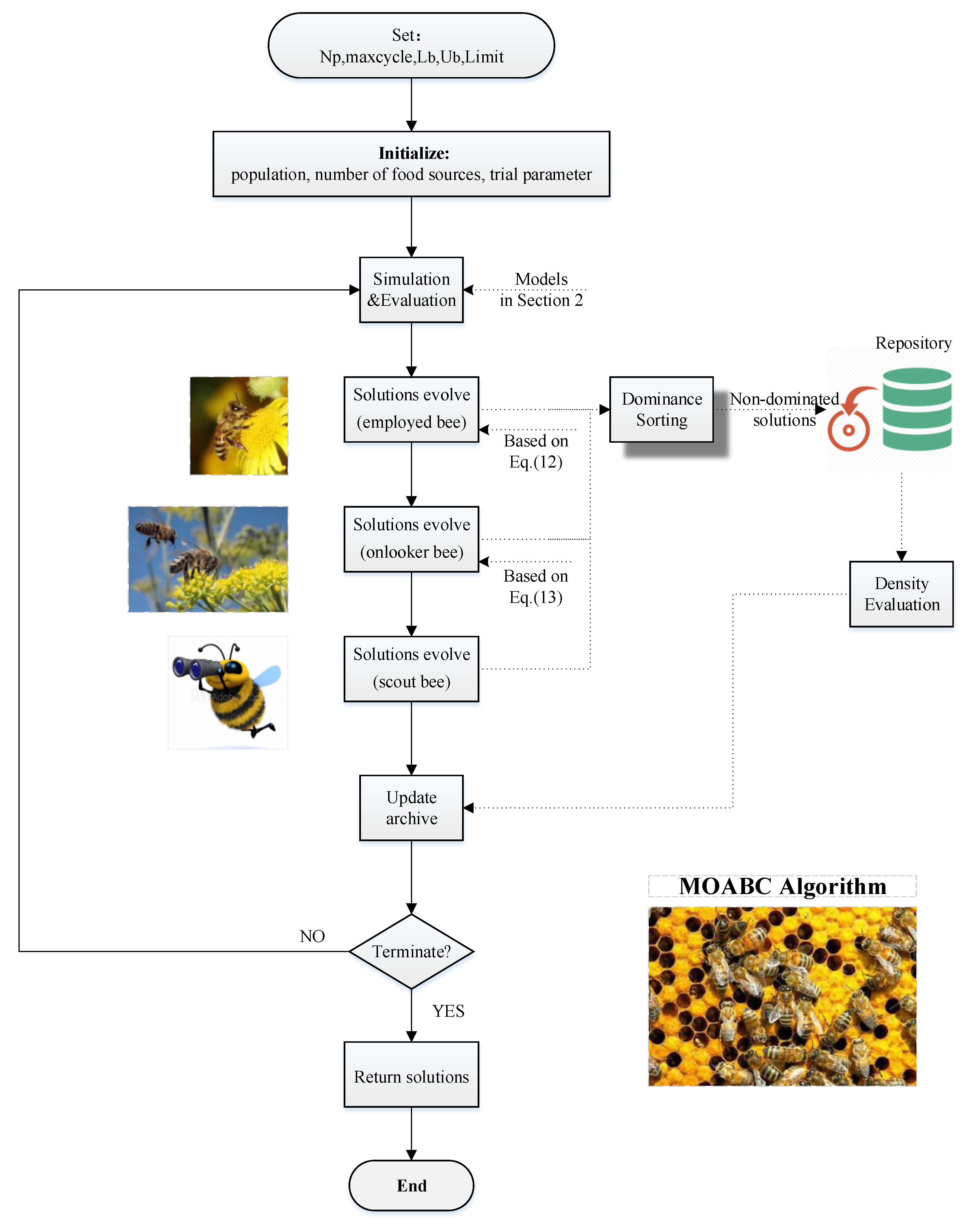
The flow chart of the artificial bee colony algorithm is shown in Figure 7. For more details and demos of MOABC, please refer to [29,30].

4.2. Q-Filter Design

This section mainly designs the Q filter for the cascaded DOB system.

For the inner-loop DOB, the following filter $Q_1(s)$ is designed,

$$Q_1(s)=\frac{1}{{(1+T_{1}s)}^4}.$$

(14)

The design principle of parameter $T_1$ could be found in [36,37,38,39] to achieve an appropriate system bandwidth. $T_1$ is set to 2 here.

In order to handle model uncertainty, we need to pay special attention to the robustness of the system. Based on Figure 5, in the nominal state, the open-loop transfer function of the inner-loop DOB is:

$$G_{L1}(s)=\frac{Q_1(s)}{1-Q_1(s)}.$$

(15)

The closed-loop robustness can be evaluated for $G_{L1}(s)$ in two popular robustness indices, sensitivity index $M_S$ and complementary sensitivity index $M_t$, defined as follows:

$$M_S=\max \left|\frac{1}{1+G_{L1}(jw)}\right|foranyw,$$

(16)

$$M_t=\max \left|\frac{G_{L1}(jw)}{1+G_{L1}(jw)}\right|foranyw.$$

(17)

The robustness constraints on the inner-loop DOB are chosen as: $M_S\le 1.4$ and $M_t\le 1.4$, which are relatively strong robustness requirements. They can be satisfied by shaping the Nyquist plot of $G_{L1}(s)$ outside the curve of each robustness index (Figure 8).

It can be seen from the figure that the designed filter $Q_1(s)$ satisfies the above robustness constraints.

For the outer-loop DOB, the following low-pass filters need to be designed,

$$Q_2(s)=\frac{1}{{(1+T_{2}s)}^2},$$

(18)

$$Q_3(s)=\frac{1}{{(1+T_{3}s)}^4}.$$

(19)

Similar to the design of Q₁, the disturbance rejection performance and robustness of the system should be taken into account when designing Q₂. Increasing the time constant T₂ will produce worse disturbance rejection performance and better robustness. The design of Q₃ mainly needs to consider the following two limitations: (1) the outer-loop robustness of cascaded DOB system and (2) the influence of the outer-loop feedback value on the inner-loop, which should not lead to the obvious oscillation of $y_1$ or the drastic change to the valve opening.

When $T_2=10$ is selected, the largest $T_3=2.6$ can be obtained by drawing the open-loop frequency response curve of the outer-loop, as shown in Figure 9. Through the following simulation, we can also know that the $T_3$ obtained here is reasonable. The robustness constraints on the outer-loop DOB are chosen as: $M_S\le 1.4$ and $M_t\le 1.4$. The equivalent open-loop transfer function of the outer-loop DOB is:

$$G_{L2}(s)=\frac{Q_3(s)Q_2(s)}{1-Q_3(s)Q_2(s)}.$$

(20)

We selected three Q₃ parameters to compare, and they were 1.5, 2.6 and 3.5, namely, candidate ‘A’, ’B’ and ’C’, respectively. Then, we made the following disturbance simulation for cascaded DOB system, adding unit step disturbance $d_1$ and $d_2$ at 1000 s and 2000 s, respectively. The simulation results are shown in Figure 10. The corresponding disturbances estimation for $T_3=2.6$ is shown in Figure 11.

It is shown that the parameters of the outer-loop filters do not affect the inner-loop disturbance rejection performance. Among the three parameters, candidate ‘A’ has a more radical disturbance suppression effect, which also leads to a drastic change in the valve opening, while ‘C’ is conservative. In summary, candidate ‘B’ is chosen as the final solution because it balances the disturbance rejection and the influence on the inner-loop. Figure 10 shows the good disturbance estimation ability of the cascaded DOB system.

4.3. Inner-Loop Controller Optimization

As mentioned earlier, for the inner-loop PI controller, both set-point tracking performance and disturbance rejection ability need to be considered. At the same time, the robustness index is considered as a constraint to reduce computational complexity.

$$M_S\le 1.6$$

(21)

We define the inner-loop PI controller in the following form:

$$G_{C1}=k_{p1}+\frac{k_{i1}}{s}.$$

(22)

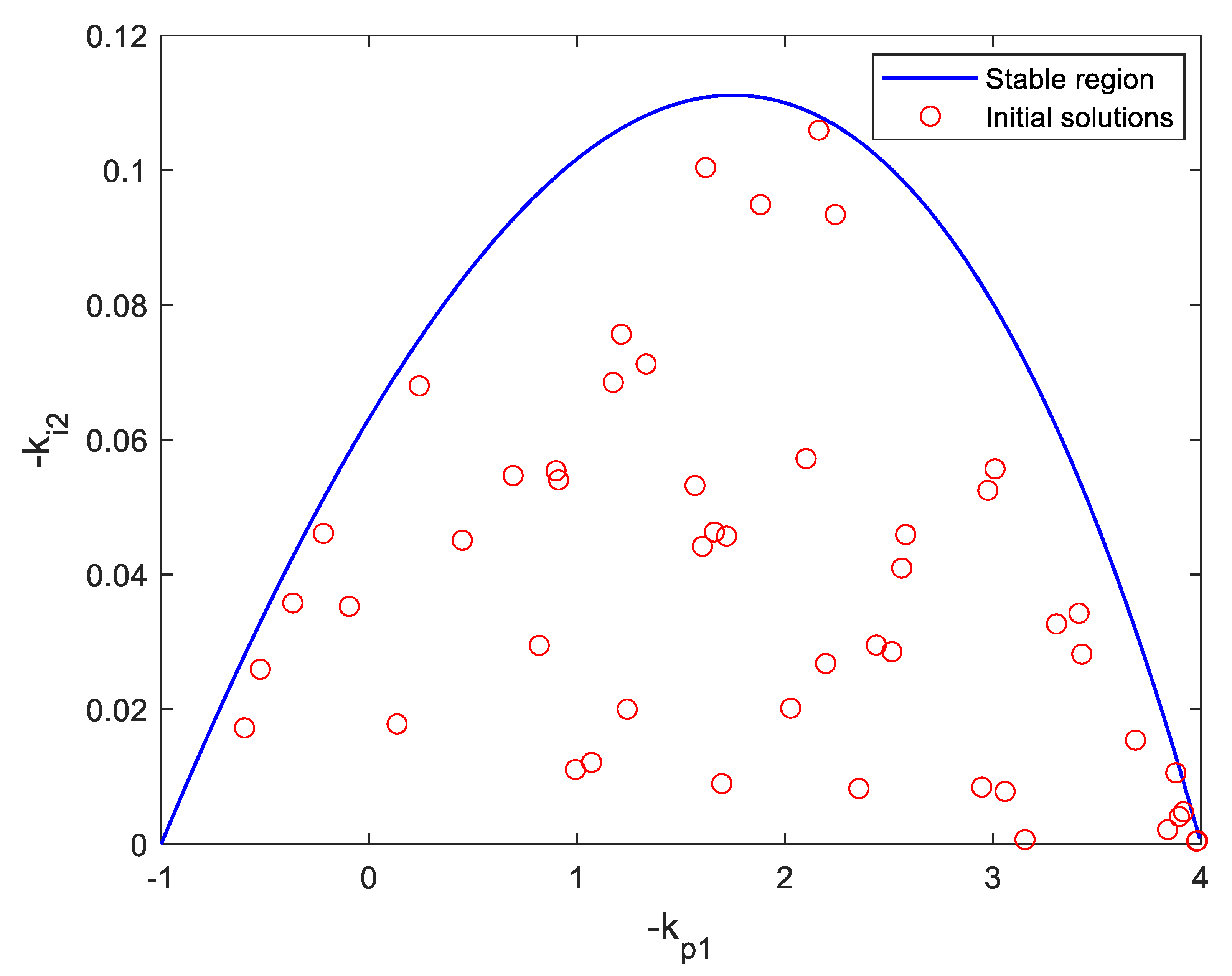
IAE₁ and IAE₂ are recorded as the IAE index of set-point tracking and disturbance rejection, respectively. As analyzed in Section 3.1, DOB has the ability to recover the nominal characteristics of the plant. Therefore, for the inner-loop, the equivalent controlled model is the nominal model of the inner-loop. So, its stable region is the same as that in [11]. It is used as the search space of inner-loop parameter optimization. As shown in Figure 12, the initial solutions of MOABC are randomly generated in the stable region.

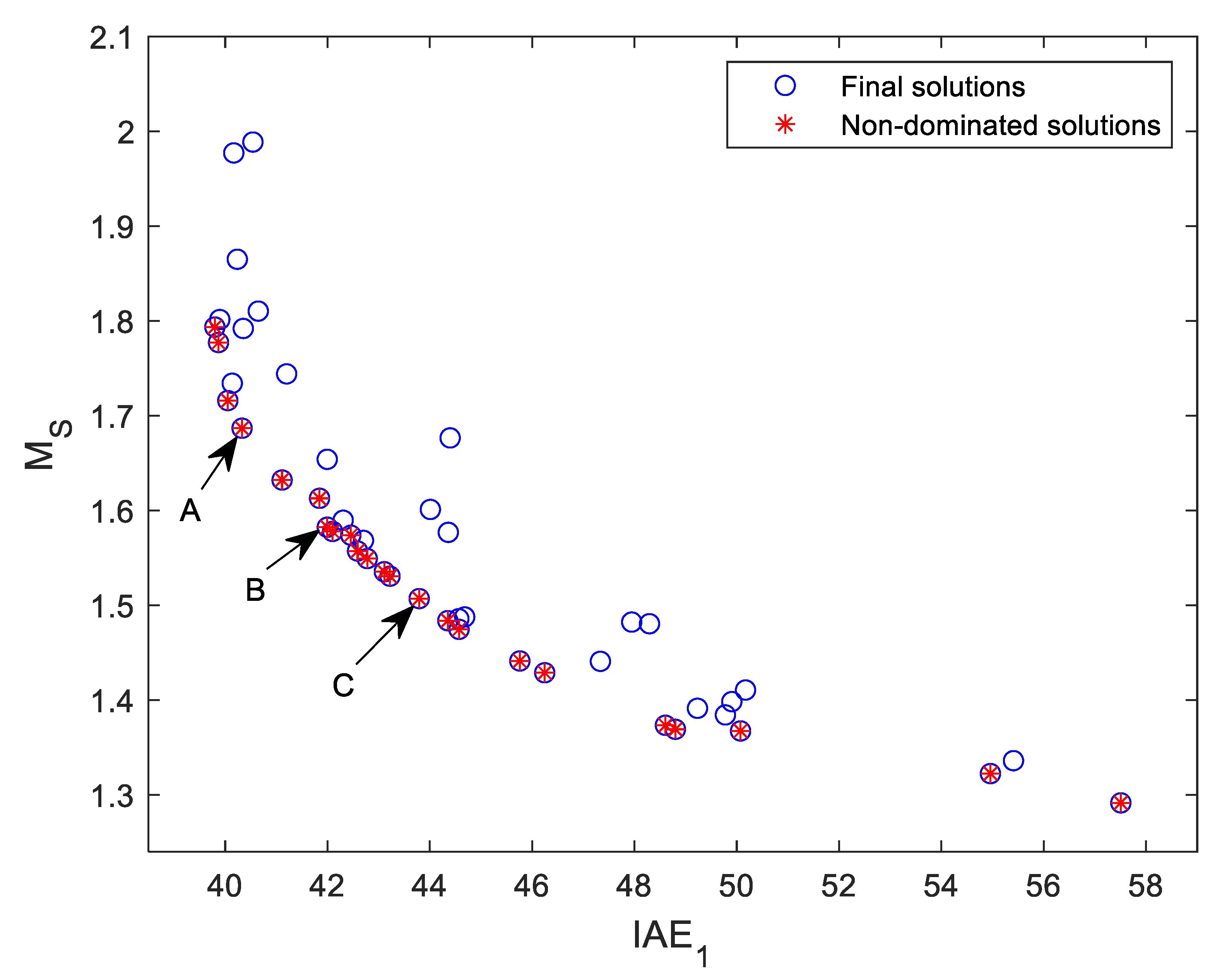
The final solutions and non-dominated solutions are shown in Figure 13. Among them, we select three candidates, ‘A’, ‘B’ and ‘C’, from the Pareto front.

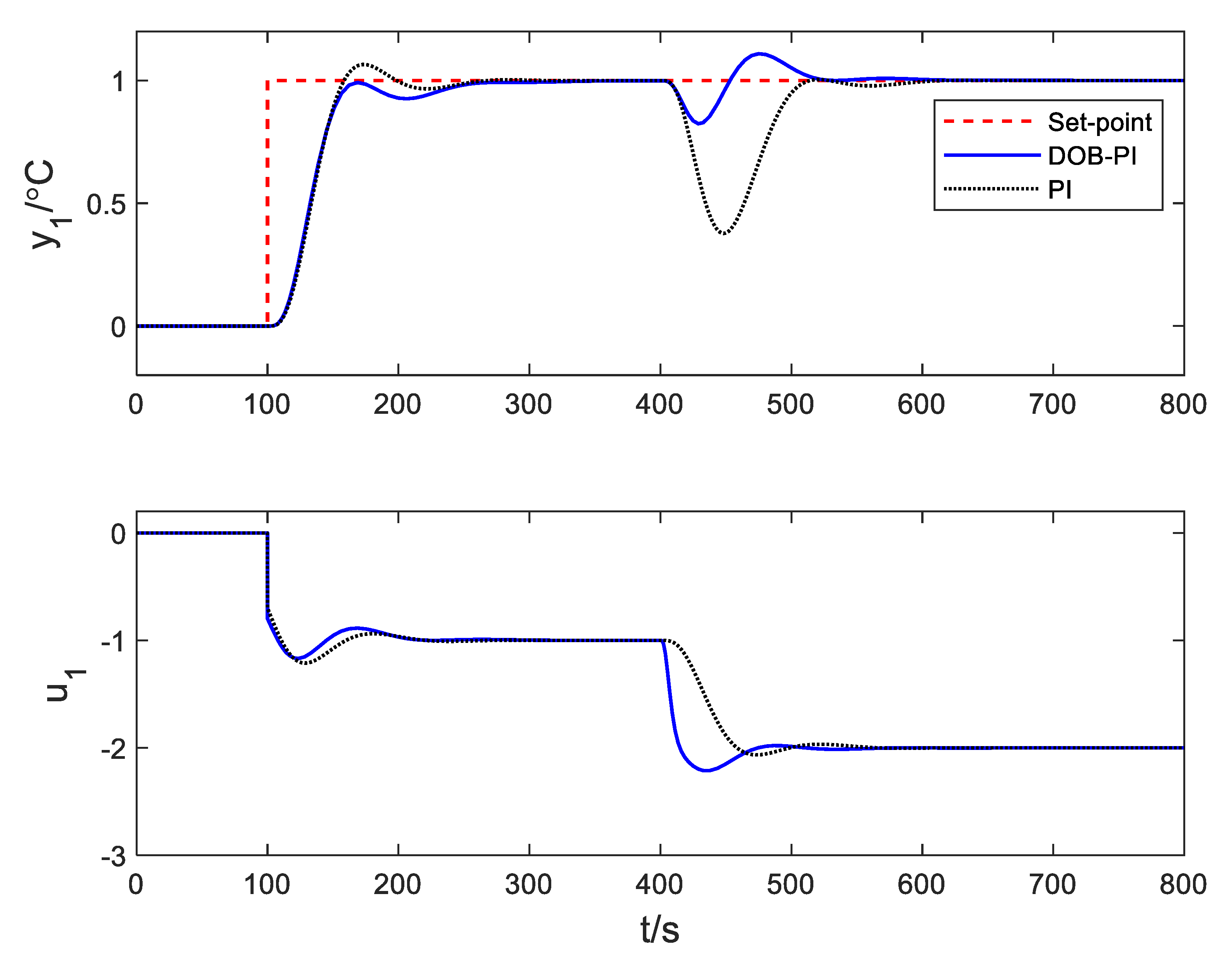
The following figure shows the relevant simulation results, in which the unit step set-point disturbance and $d_1$ disturbance are added at 100 s and 400 s respectively (Figure 14). The controller parameters and related indicators of the three non-dominated inner-loop controllers are shown in

Table 1. Comparison of indices for the three non-dominated inner-loop controller candidates of cascaded DOB-PI.

Candidates	kp1	ki1	T1	IAE1	IAE2
A	−0.72	−0.027	2	36.98	9.81
B	−0.79	−0.026	2	38.78	9.63
C	−0.84	−0.025	2	40.75	9.54

.

It can be seen that, the parameters of the PI controller have almost no effect on inner-loop disturbance suppression, which also proves that the disturbance suppression of the inner-loop is mainly undertaken by DOB. The selected solution ‘B’ is a tradeoff between the set-point tracking performance and the disturbance rejection.

4.4. Outer-Loop Controller Optimization

For the outer-loop controller design, the main consideration is the disturbance rejection performance because the set-point of SST is generally a constant. On the other hand, in order to ensure the robustness of the control system, the robustness index is optimized as another objective. Therefore, the objective functions of outer-loop multi-objective optimization are the IAE index in terms of disturbance $d_2$ and the M_S index.

For the outer-loop, we considered the following PI controller:

$$G_{C2}=-\left(k_{p2}+\frac{k_{i2}}{s}\right).$$

(23)

Similar to the analysis in Section 4.3, the outer-loop DOB can also recover the nominal model of the plant, so the stable region of the outer-loop PI controller is the same as that in [11]. It should be noted that since the outer-loop disturbance suppression is mainly undertaken by DOB, the integral value obtained by optimization is close to 0, so in order to ensure the steady-state of the closed-loop system is error free, the minimum integral parameter is set to 0.003. At this point, the controlled model of the outer-loop is as follows:

$$G_{e2}=\frac{G_{C1}{G}_1}{1+G_{C1}{G}_1}{G}_2=G_{e1}{G}_2.$$

(24)

As can be seen from Figure 15, the final solutions of the outer-loop controller parameter optimization are all in the stable region.

Figure 16 shows the final solutions and non-dominated solutions of multi-objective optimization. Among them, we select three candidates, ‘A’, ‘B’ and ‘C’, from the Pareto front.

The following figure shows the relevant simulation results, in which a unit step disturbance $d_2$ is added at 100s (Figure 17). The controller parameters and related indicators of the three non-dominated outer-loop controllers are shown in

Table 2. Comparison of indices for the three non-dominated outer-loop controller candidates of cascaded DOB-PI.

Candidates	kp2	ki2	T1	T2	T3	IAE	MS
A	0.93	0.003	2	10	2.6	40.3	1.69
B	0.81	0.003	2	10	2.6	42.0	1.58
C	0.71	0.003	2	10	2.6	43.8	1.51

.

It can be seen that, there is little difference between the three PI controllers, due to the strong disturbance rejection ability of cascaded DOB. The selected solution ‘B’ is the control parameter that has the minimum IAE index under the certain robustness index ($M_S\le 1.6$).

5. Comparison and Mismatch Test

This section verifies the superiority and robustness of the proposed control strategy through comparison with conventional cascaded PI controllers and mismatch simulations.

In Section 5.1, the parameters of the conventional inner and outer-loop PI controller are taken from multi-objective optimization solution in [11]. In Section 5.2, control performance in the case of time constant and the gain mismatch of the inner and outer-loop are compared, respectively (based on the control structure of Figure 6).

5.1. Comparison with Cascaded PI Scheme

5.1.1. Inner-Loop Simulation

The same simulation is carried out using the optimized DOB-PI and PI controller parameters. The results are shown in Figure 18, and the related indicators are shown in

Table 3. Indices comparison of inner-loop controller.

Control Strategy	kp1	ki1	IAE1	IAE2
DOB-PI	−0.79	−0.026	38.78	9.63
PI	−0.7	−0.03	36.6	35.6

.

It can be seen that the inner-loop has a significant improvement in disturbance rejection performance. The setpoint tracking ability is slightly worse due to the relatively small integral effect.

5.1.2. Outer-Loop Simulation

A similar comparative simulation is carried out in the outer-loop, and the results are shown in Figure 19. The related indices are summarized in

Table 4. Indices comparison of outer-loop controller.

Control Strategy	kp2	ki2	IAE	MS
Cascaded DOB-PI	0.81	0.003	42.0	1.58
Cascaded PI	0.53	0.0055	184	1.59

.

It can be seen that the cascaded DOB-PI control strategy has better disturbance rejection performance under the same robustness index. A smaller SST fluctuation means that the power plant can participate in a wider range of load dispatching, which is conducive to the consumption of renewable energy.

5.2. Mismatch Simulations

This part carries out the control simulation under the condition of inner- and outer-loop model mismatch, in order to verify the robustness of the control system against model uncertainties.

5.2.1. Inner-Loop Model Mismatch

Simulations are made under the nominal case and model mismatch cases. Two model mismatch conditions for $G_1(s)$ are considered: process gain varies from 1 to 1.3 and time constant varies from 9 to 11. The simulation results are shown on Figure 20. A unit step command disturbance and $d_1$ disturbance are added at 100 s and 400 s, respectively.

As can be seen from the figure, the inner-loop can still achieve a good control performance when the gain change is about 30%. When the time constant changes to about 20%, $y_1$ oscillates obviously but remain stable. In particular, there is no obvious change in disturbance rejection. This also shows the superiority of the DOB-PI control strategy in disturbance suppression.

5.2.2. Outer-Loop Model Mismatch

Similarly, simulations are made under the nominal case and model mismatch cases for the outer-loop. Two model mismatch conditions for $G_2(s)$ are considered: process gain varies from 1.5 to 2 and time constant varies from 60 to 80. The simulation results are shown in Figure 21. A unit step disturbance $d_2$ is added at 100 s.

It can be seen that, when the gain varies to 2, the control effect of $y_1$ and $y_2$ changes little, but the valve opening $u_1$ increases for a short time. When the time constant varies to 80, due to the slower dynamic, $y_1$ and $y_2$ fluctuate obviously but still remain stable.

Through the above comparison and simulation, the superiority and robustness of the proposed control strategy are verified.

6. Conclusions

In this paper, the control difficulties of SST caused by unknown disturbances and model uncertainties are introduced based on the description of an SST system. In order to improve the control performance, a cascaded DOB-PI control strategy is proposed in this paper. The multi-objective optimization models of inner- and outer-loop PI controllers are established to achieve the best control performance on the premise of robustness.

The optimized Pareto front and simulation results show that the cascaded DOB-PI control strategy can significantly improve the disturbance rejection performance of the SST control system while maintaining its strong robustness and traditional cascaded control structure. Due to the wide applicability of DOB, this control structure is suitable not only for the SST control system, but also for other cascaded systems affected by disturbances. At the same time, from the comparison in Section 5.1.1, we can see that the optimal solution in this paper sacrifices part of the inner-loop tracking performance. Compared with the traditional cascaded PI control system, the control structure adopted in this paper is more complex. The design method of the Q filter can be further improved with reference to advanced design methods, such as $H_{\infty }$ optimization.

Compared with the traditional cascaded PI scheme, the proposed SST control strategy has good disturbance suppression performance and promising prospects for practical application when it comes to increasing demand for more renewables in the power grid.