Abstract
CO2 emissions account for 80% of greenhouse gases, which lead to the largest contributions to climate change. As the problem of CO2 emission becomes more and more prominent, research on sustainable technologies to reduce CO2 emission among environmental loads is continuously being conducted. In-situ production of precast concrete members has advantages over in-plant production in reducing costs, securing equal or enhanced quality under equal conditions, and reducing CO2 emission. When applying in-situ production to real projects, it is vital to calculate the optimal quantity. This paper presents a dynamic optimization model for estimating in-situ production quantity of precast concrete members subjected to environmental loads. After defining various factors and deriving the objective function, an optimization model is developed using system dynamics. As a result of optimizing the quantity by applying it to the case project, it was confirmed that the optimal case can save 7557 t-CO2 in CO2 emissions and 6,966,000 USD in cost, which resulted in 14.58% and 10.53% for environmental loads and cost, respectively. The model developed here can be used to calculate the quantity of in-situ production quickly and easily in consideration of dynamically changing field conditions.
1. Introduction
Due to climate change, problems such as droughts, heatwaves, and rising sea levels are globally occurring [1]. One of the biggest causes of climate change is greenhouse gas [2], and international regulations on greenhouse gas emissions are being strengthened [3]. CO2 accounts for 80% of greenhouse gases, and the problem of CO2 emission becomes more and more prominent [4]. In particular, research on sustainable technologies to reduce CO2 emission among environmental loads is continuously being conducted [5,6,7,8,9]. The construction industry is recognized as a major cause of environmental pollution [10], and it is important to quantify and evaluate the environmental load.
In studies related to the calculation of environmental loads of construction, Tae et al. evaluated the CO2 generated during the life cycle of a building and its economic efficiency to assess the environmental loads and costs of buildings that use plaster board drywall [11]. Priatla et al. proposed a methodology to quantify CO2 emissions by life cycle in water supply construction projects [12]. Park et al. studied correlation analysis between the environmental load computed through life cycle assessment (LCA) using the database of national highway construction cases and the inventory of available information that can be extracted in the road planning stage [13]. Lee et al. developed and validated an environmental load estimating model for the New Austrian Tunneling Method (NATM) tunnel based on the standard quantity of major works in the early design phase [10]. These studies were conducted to develop decision-support tools using quantified environmental loads, or to evaluate environmental loads by applying life cycle cost (LCC) or environmental valuation methodologies.
In-situ production of precast concrete (PC) members not only reduces the cost by 14.5–39.4% compared to in-plant production, but can also result in equal or enhanced quality under equal conditions [14,15,16,17,18]. Through an experiment in which the amount of CO2 emission reduction was analyzed according to the increase in quantity, it was proved that in-situ production is an eco-friendly technology with a high CO2 reduction effect [19]. However, in order to apply in-situ production to a project, additional research is needed to calculate the optimal quantity considering the environmental load.
However, it is difficult to produce all quantities in situ due to various field constraints, as well as the given time. The in-situ production quantity is affected by various factors, such as lead-time, number of molds, and number of cranes [17,20]. Although quantity is an important factor that determines the in-situ production scale, it is difficult to estimate it because it is indirectly affected by most of the influencing factors. Therefore, a simple method is necessary to calculate the optimal quantity to apply in-situ production in real projects.
Therefore, the objective of this paper is to develop a dynamic optimization model for estimating the in-situ production quantity of PC members subjected to environmental load. By defining various factors and deriving the objective function, the optimization model is developed using system dynamics and then applied to a case project for verification. The model developed here can be used to calculate the possible quantities of in-situ production quickly and easily in consideration of dynamically changing field conditions.
This study is carried out as follows.
- (1)
- The influencing factors of in-situ production for CO2 emission are defined.
- (2)
- The development process for the optimization model is explained.
- (3)
- The objective function to minimize CO2 emission is derived.
- (4)
- A dynamic optimization model reflecting the objective function is developed.
- (5)
- The environmental loads for the members applied to the actual in-situ production are calculated.
- (6)
- The optimization model is simulated using Monte Carlo simulation.
- (7)
- The control range of each influencing factor is derived using system dynamics.
- (8)
- Dynamic optimization model is applied in the case project for verification.
2. Preliminary Study
Under equal production conditions, it was verified through experimental studies that in-situ production of PC members secures equivalent or enhanced quality compared to in-plant production while significantly reducing costs [17,18,20,21]. Lee studied the management model and necessary conditions for in-situ production of composite PC members, and suggested cost, quality, process, resources, and safety management as management factors [22]. Park et al. studied the manufacturing technology for in-situ production of ultra-high-strength PC piles and suggested optimal production conditions through experimental production [23]. Won et al. studied the energy efficiency of in-situ production of PC members using steam curing and suggested necessary equipment and production concepts [24]. Lim et al. introduced a detailed management process through a case study of in-situ production and showed that the cost effectiveness ratio increased as the quantity increased [18]. Kim et al. presented the embedded energy efficiency of their proposed precast concrete frames based on the material, structure, and construction characteristics [25]. These studies analyzed specific plans for in-situ production of PC members and items to be considered when planning and showed that they were advantageous in terms of quality and cost of in-situ production.
Recently, CO2 has been one of the most important causes of global climate change [2], and a method that can apply in-situ production of PC members is needed. Several studies were conducted to reduce CO2 emissions of the PC method. Dong et al. showed that the PC method is a way to reduce carbon emissions by comparing to the cast in-situ construction method through experiments using life cycle assessments [26]. Yepes et al. proposed a methodology to optimize CO2 emissions when designing a PC road and developed a hybrid glowworm swarm optimization algorithm [27]. Kim and Chae presented that a considerable amount of CO2 is emitted during the steam curing stage when making PCs, and proposed a method of evaluating CO2 emissions throughout the PC life cycle using life cycle assessment [28]. Lim et al. calculated CO2 emissions with the LCA method through an experimental study of in-situ production and determined that the amount of CO2 emission reduction increases as the quantity of in-situ production increases [19]. These studies were reviewed from the eco-friendly perspective for field application through optimization and evaluation methods for the existing PC method’s CO2 emissions. In addition, it was confirmed that it is advantageous to apply in-situ production in terms of CO2 emissions, but more research on minimizing CO2 emissions is needed.
Several studies used system dynamics in the production and installation of PC members to analyze influencing factors. Tan et al. applied the Pull-Driven Scheduling (PDS) simulation technique for the Singapore Light Rail Transit (LRT) project to produce PC members. The installation process was dynamically analyzed [29]. Ballard et al. conducted a study to improve the productivity of in-plant production for PC members using dynamic analysis techniques based on the measured data [30]. Cho et al. expressed the production, transportation, and construction process for PC-structured apartment houses as an Entity–Relationship Diagram (ERD) [31]. Lim et al. analyzed the factors that influence the calculation of the in-situ production volume and applied the developed simulation model to six scenarios to derive the in-situ production volume [20]. These papers showed that the dynamic relationships of various influence factors have been considered, and more research using them is being conducted. Therefore, in order to minimize CO2 emissions, this paper aims to calculate the optimal quantity considering the dynamic relationship of various factors such as lead-time, number of molds, and number of cranes.
3. Methodology for the Optimization Model
The authors describe system dynamics and the Monte Carlo simulation method as applied techniques for developing an optimization model for estimating CO2 emissions, followed by the definition of influence factors for in-situ production of PC members with details in step-by-step processes. Then, a dynamic optimization model is developed to minimize environmental loads in the sequence of a generation model, simulation model, and optimization model.
3.1. Applied Techniques for Simulation
3.1.1. System Dynamics
In carrying out in-situ production of PC materials, there is a limit to the complexity of the relationship between these influencing factors, which is why it is difficult to clarify this with general static analysis [17]. Static analysis is used because the one-way independent variable affects the dependent variable, it expresses the causes and effects of temporary events, and it views things from a partial perspective. Therefore, a system dynamics technique is needed as a means to grasp and quantify the dynamic relationship between influencing factors.
System dynamics can be defined as follows: (1) Rather than obtaining estimated values of a one-time event or variable, more attention is paid to what kind of dynamic change tends to occur over time in the variable of interest. (2) All phenomena are viewed from the perspective of an internal and cyclical closed-loop thinking, and are understood to be caused by circular dynamic interactions [32]. (3) The research focuses on the process of change and how it is actually happening. In other words, system dynamics is a methodology for understanding complex systems, and is a research methodology that explains the changes in the system over time, focusing on the causal relationship and the feedback relationship [33,34].
3.1.2. Monte Carlo Simulation
The dynamic optimization model was developed using the Powersim Studio 10 Expert program and the simulation was run by utilizing influencing factors such as in-situ production quantity, lead-time, number of molds, and number of cranes. Many values for factors must be derived through simulation, and control ranges for the values need to be set. A random number that follows the probability distribution for each factor is generated using Monte Carlo simulation. Using a computer program is the most effective way to generate a series of random numbers [35]. Monte Carlo simulation is performed by generating 100,000 random numbers, assuming a deviation of 0.1. Various values are presented by random numbers for each variable generated through Monte Carlo simulation. In other words, it attempted to overcome the mathematical limitations of the deterministic method by using the probabilistic method [36].
3.2. Definition of Influencing Factors for In-Situ Production
In-situ production of PC members is carried out in the same manner as in-plant production—applying demolding oil, pouring concrete, finishing the surface of the member, curing, demolding, and yard stocking [21]. In-situ production can be carried out at the same level as the factory by placing the assembled reinforcing bars in the steel formwork, as shown in Figure 1a. As shown in Figure 1b, steam curing is performed using a boiler, and the cured PC member is stacked. All processes are accomplished by establishing a production plan that can be supplied in the just-in-time delivery method of PC members according to the installation plan.
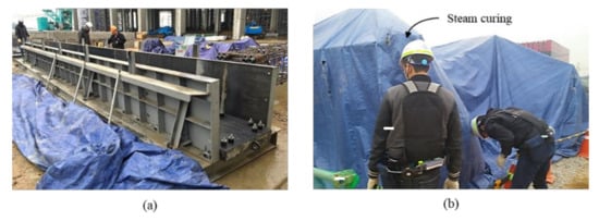
Figure 1.
Major process of in-situ production: (a) manufactured steel mold [20]; (b) steam curing [18].
A survey conducted by Lim found that quantity was the most important influence factor for in-situ production [17]. The importance of influence factors was in the following order: number of cranes, number of molds, lead-time, yard stock area, production area, production cycle, erection cycle, material and traffic control, and crane location. In the study, only the factors that directly affect the calculation of the in-situ production quantity were considered by reflecting the results of the existing studies and the field application cases, and five influencing factors were selected, including cost, quantity, lead-time, number of molds, and number of cranes. Figure 2 is a causal loop diagram illustrating in-situ production cost, quantity, lead-time, number of molds, and number of cranes using system dynamics.
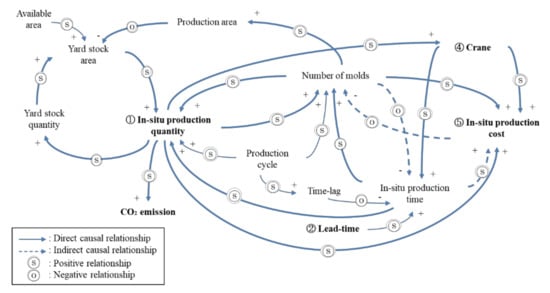
Figure 2.
Causal loop diagram for estimating in-situ production quantity.
Details for each influencing factor are as follows.
- In-situ production quantity: Since CO2 emissions can be calculated only by the quantity, quantity is the factor that has the greatest influence on CO2 emissions, and is a key influence factor and result of this study. Equation (1) shows how the quantity can be calculated using the in-situ production time, number of molds, and production cycle. In Figure 2, the in-situ production quantity affects the stock volume, and the stock quantity is determined by the difference between the accumulated production quantity and the accumulated installation quantity. As the stock volume increases, the yard stock area increases, and as the yard stock area increases, the in-situ production quantity can be increased.where QSITU: in-situ production quantity (unit); TSITU: in-situ production time (day); NMOLD: number of molds (unit); TPC: production cycle time (day).
- Lead-time: When applying in-situ production, a separate process plan for the site is required. Figure 3 shows that the lead-time is the time of in-situ production in advance before the PC member is installed and is the period from the start of production of the PC member to the start of installation. Considering the curing period, not all PC members can be produced during the installation period, so members must be produced in advance [17,20]. As the in-situ production time increases, the amount of in-situ production available increases, so it is important to secure lead-time, as shown in Figure 2. The lead-time can be calculated using the production cycle, quantity during lead-time, and number of molds, as shown in Equation (2).where TLEAD: lead-time (day); TPC: production cycle time (day); QSLi: in-situ production quantity during lead-time (unit); NMTi: number of mold types (unit); i: number of mold types (1, …, n).
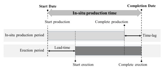 Figure 3. Calculation of in-situ production time [20].
 - Number of molds: As the number of molds increases, the quantity of production per unit of time is increased, resulting in a strong effect of shortening the time, while the cost of in-situ production increases rapidly. The reason is that the steel mold manufacturing cost is high. PC members of various sizes cannot be produced with molds of the same size. Table 1 shows five mold types classified according to the size of the member. Figure 2 shows that as the in-situ production quantity increases, the number of molds increases, and the number of molds affects the production area. The number of molds also affects the in-situ production quantity, so they affect each other. Since the in-situ production cost indirectly increases as the amount of time increases, it is necessary to calculate an appropriate number of molds through a feedback routine. The number of molds is a key influence factor in calculating the quantity of in-situ production, considering the time and cost. In Equation (3), the number of molds can be calculated by using in-situ production quantity, production cycle, and time.where NMOLD: number of molds (unit); QMOLDi: in-situ production quantity of each mold type (unit); TPC: production cycle time (day); TSITU: in-situ production time (day); i: number of mold types (1, …, n).
 Table 1. The shapes of precast concrete (PC) members.
 - Number of cranes: The large-scale building covered in this paper has a large floor area but not a high number of floors, making it difficult to use a tower crane, so a mobile crane was used. A crane is used to move the module and to lift and install the PC members. Equation (4) shows that the number of cranes can be calculated by dividing the installation time by the product of the unit usage time per member and the number of installation members, and the number of cranes are an integer equal to or greater than 1.where Ncrane: number of cranes (unit); TUE: unit erection time (day); QSITU: in-situ production quantity (unit); Terec: erection time (day).
- In-situ production cost: The cost is less than the in-plant production cost and is proportional to the quantity and number of molds. If the cost is not satisfied, in-situ production cannot be applied, so it is a limiting condition for minimizing CO2 emission. If the total production cost of PC components is high, the in-situ production volume, which is lower than the in-plant production cost, is increased [16]. Figure 2 shows that all influence factors affect cost and can finally be collected. Equation (5) shows that cost can be calculated by the number of mold types, unit mold production cost for mold type, in-situ production quantity, and unit PC member production cost.where CSITU: in-situ production cost (USD); NMOLDi: number of mold types (unit); CMOLDi: unit mold production cost for mold type (unit); QMOLDi: in-situ production quantity for mold type (unit); CPRODi: unit PC member production cost for mold type (USD); i: number of mold types (1, …, n).
3.3. Dynamic Optimization Model to Minimize Environmental Loads
The dynamic optimization model was developed sequentially through the generation model and simulation model. The generation model determines one case, and the simulation model derives the control range through simulation. The optimization model is used to find the most suitable value for the field condition among simulated values. This development process is shown in Figure 4.
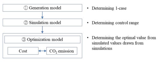
Figure 4.
Development process for the optimization model.
3.3.1. Generation Model
The generation model determines one case by deriving the in-situ production cost and time for various influence factors. For instance, the 72 columns of in-situ production conducted in this experimental study are a generation model. Using the quantity calculated based on the design drawings, the CO2 emissions for the 72 columns generated during in-situ production of total PC members were calculated. Influencing factors each have one value, and Figure 5 shows the mathematical connection of the relationship between influencing factors and CO2 emissions. That is, an equation defines five influencing factors of in-situ production cost, quantity, lead-time, number of molds, and number of cranes, and calculates CO2 emissions by substituting the influence factors into each equation. This generation model can be expressed as shown in Figure 5. All the influence factors have a dynamic relationship with each other, as shown in Figure 2.
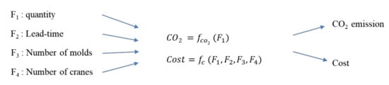
Figure 5.
Concept of the generation model.
In this study, CO2 emission sources, such as material, oil, electricity, and transportation, are classified and calculated for the analysis of the CO2 emission reduction effect on in-situ production. After defining basic units of CO2 emission or estimation equations for each source in advance, the quantity of CO2 emissions generated by in-plant production is calculated using the quantity of sources. Next, the CO2 emissions by in-situ production are calculated and compared with in-plant production. In order to calculate the material use, each basic unit of CO2 emission per material quantity is used [37]. Concrete 140 kg-CO2/m3 and Steel 3500 kg-CO2/t can be used to calculate CO2 emissions. In the studies of Hong et al., Lee et al. and Lim et al., the CO2 emissions generated in the construction stage of the building were calculated in the same way [19,38,39,40,41,42].
For the CO2 emissions of the erection process, CO2 emissions according to the use of oil and electricity must be calculated. Kim et al. analyzed using the LCA technique and proposed a CO2 emission regression equation at the construction stage [37]. Since this regression equation has a gross floor area as a variable, it is easy to estimate CO2 emission according to oil use and power consumption. First, the equation for calculating the CO2 emissions of the construction work according to the use of oil in the construction stage is the same as Equation (7), which can be calculated using Equation (6), an equation for calculating energy consumption [37]. The oil use of in-situ and in-plant production was the same with the same production conditions. The equation for calculating CO2 emissions at the construction stage according to power consumption is the same as Equation (9), which can be calculated using Equation (8), an equation for calculating energy consumption. CO2 emissions by transportation equipment use are only applicable when moving PC members manufactured at the plant to the construction site. Unlike in-situ production, in-plant production requires transport of members, and basic units of CO2 emission are 0.464 kg-CO2/ton·km and 31.080 kg-CO2/number of units of equipment [37].
where ECO: energy (oil) consumption during the construction stage; Af: total floor area (m2); QCO2O: CO2 emissions based on oil use in the construction stage (t-CO2); ECE: power consumption in the construction stage; QCO2E: CO2 emissions based on power consumption in the construction stage (t-CO2).
3.3.2. Simulation Model
The simulation model was created based on the generation model [43]. The five influencing factors, such as in-situ production quantity, lead-time, number of molds, and number of cranes, can derive a range value according to the site conditions. The dynamic optimization model was developed using the Powersim Studio 10 Expert program in this paper and can be simulated using the derived influencing factors. Various values are presented by random numbers for each variable generated through the Monte Carlo simulation by using a number of cases as a result of the influencing factor, cost, and the minimum value, which is the control range of CO2 emissions. The minimum value (Min) and maximum value (Max) can be derived, and Figure 6 is a schematic diagram.
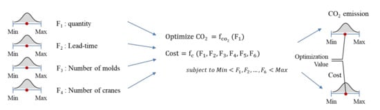
Figure 6.
Concept of the simulation model.
3.3.3. Optimization Model
When the simulation model is developed, an optimization model is created using the derived values. The optimization model calculates one most appropriate value from the Min–Max of CO2 emission, which is obtained from the results of the simulation model. It is possible to derive appropriate values of in-situ production cost, quantity, lead-time, number of molds, and number of cranes, which are influencing factors corresponding to optimal CO2 emissions. Figure 7 is a schematic of the optimization model, and it can be derived using the Powersim Studio 10 Expert program.
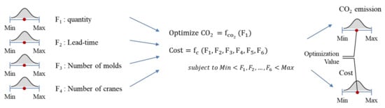
Figure 7.
Concept of the optimization model.
Environmental load assessment measures whether CO2 emission is minimized within the range possible for in-situ production. Environmental loads can be calculated for in-situ and in-plant production. The larger the difference between these values, the more CO2 emissions are minimized. The cost, time, and yard stock area are within the allowable range. Equation (10) is an objective function and boundary condition to minimize environmental loads. Among the various values generated through the Monte Carlo simulation within the range satisfying these constraints, the maximum difference between in-plant and in-situ production for environmental loads is derived. Equations (11) and (12) are methods of estimating environmental loads for in-situ and in-plant production, respectively. They can be calculated by multiplying the quantity by the sum of the values for each item of material use, oil use, electronic use, and transportation equipment use. Transportation equipment use is calculated only in the case of in-plant production, and these values can be accumulated by member type.
where QCO2P: CO2 emissions of in-plant production (t-CO2); QCO2S: CO2 emissions of in-situ production (t-CO2); Creq: required cost (USD); Cavail: available cost (USD); Treq: required time (month); Tavail: available time (month); Areq: required area (m2); Aavail: available area (m2); QPi: in-plant production quantity of mold types (t-CO2); QCO2M: CO2 emissions of material use (t-CO2); QCO2O: CO2 emissions of oil use (t-CO2); QCO2E: CO2 emissions of power consumption (t-CO2); QCO2T: CO2 emissions of transport equipment use (t-CO2); QSi: in-situ production quantity of mold types (t-CO2); i: number of mold types (1, …, n).
4. Development of the Dynamic Optimization Model
Based on the previously mentioned causal loop diagram and the dynamic optimization model, the cost and CO2 emission simulation models were created using the Powersim Studio 10 Expert program. The mold type derived based on the previously analyzed PC column and PC beam shape was applied.
4.1. Cost Model
The cost simulation model created for one mold type is shown in Figure 8. From the cost model, the in-situ production time is calculated using time-lag, lead-time, installation start date, and installation completion date (A). By entering the production cycle of two days and five working days per week, the number of parts per week is calculated, and the number of units of production is applied to the calculation of the number of molds together with the quantity and the in-situ production time (B). Material cost, labor cost, and equipment cost can be calculated using these calculated values.
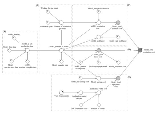
Figure 8.
Cost estimation simulation model (mold type 1 for in-situ production); in-situ production time (A), production time (B), total material cost (C), total labor cost (D), total equipment cost (E).
Material cost is calculated by dividing into PC member production cost and mold cost (C). PC member production cost is calculated using the material cost for the production of one member composed of concrete and rebar, the number of parts produced per week, and the quantity of production, and the mold cost can be calculated using the number of molds and the unit cost of the mold. Labor cost is calculated as the input manpower during the period in which the mold was used. The labor cost is calculated using the number of molds, the amount of manpower, the number of working days per week, and the labor unit cost (D). Equipment cost is classified into curing cost and crane rental cost (E). Curing cost is calculated using the number of molds and curing unit cost. Since the stack quantity is determined by the difference between the production quantity and the installation quantity occurring over time, the crane utilization period is calculated based on the quantity of the yard. The crane rental cost is determined by the crane utilization period, unit rental cost, and number of units. The total production cost for one mold type is calculated by summing the material cost, labor cost, and equipment cost. For the production of PC members, the total in-situ production cost is calculated by summing the production cost for each mold type. The calculated in-situ production cost is then compared with in-plant production to determine whether the cost is reduced.
4.2. Environmental Load Model
The environmental load simulation model developed for one mold type is shown in Figure 9. From the perspective of in-plant production, environmental load is calculated by dividing into material use (B), oil use, electric use (C), and transport equipment use (D). First, in (A) of Figure 9, material use is calculated by summing reinforcement works of high-tensile deformed-bar (HD) 13, HD 16, HD 19, super-high-tensile deformed-bar (SHD) 22, SHD 32, SHD 35, embedded steel, etc. by checking the drawing to calculate the rebar weight of the member corresponding to mold type 1. Material use is calculated using this rebar weight, and the amount of concrete is calculated by checking the drawing, the actual steel form used, and the CO2 base unit of steel and concrete. Oil use and electric use are calculated using the total floor area and number of total members, while transport equipment use is calculated using trailer size, distance from site to factory, CO2 emission base unit of distance, and transport equipment use.
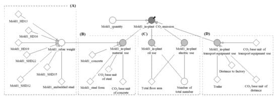
Figure 9.
Environmental load simulation model (mold type 1 for in-plant production); material use (A), in-plant production material use (B), oil and electric use (C), transport equipment use (D)
Total CO2 emissions are calculated by summing material use, oil use, electric use, and transport equipment use. If the total CO2 emissions for one mold type of in-plant production are calculated, the total in-plant production CO2 emissions are calculated by summing the production cost for each mold type. CO2 emissions for in-situ production are calculated excluding the use of transport equipment in all processes. The calculated in-situ production CO2 emissions can be compared with the in-plant production to determine the degree of CO2 emission reduction.
5. Application of the Dynamic Optimization Model
5.1. Estimation of Environmental Loads for the Case Study
5.1.1. Estimation of In-Situ Production Quantity
A case study was selected to apply the developed dynamic optimization model. The case project is located in Cheonan-si, Chungcheongnam-do, Republic of Korea, and has a site area of 53,055.60 m2, building area of 42,406.07 m2 (246 m long × 178 m width), and total floor area of 167,614.82 m2. The case project has a scale of four stories above the ground, with 2–4 stories above the ground with a PC structure, a core structure of reinforced concrete, and a roof structure of steel. Therefore, this study targets the 2–4 floors above ground because they are built with a PC structure. A total of 72 members are produced in-situ in the case project. The members to be constructed are columns, girders, and slabs. However, the members capable of in-situ production are limited to columns and girders that require a small production area. The columns and girders are thin and long, so the production space is not wide, but slabs require a large space, making in-situ production difficult in a limited area.
The number of PC members capable of in-situ production at the case site is 1,004 columns and 1252 girders, a total of 2256 members. Table 2 shows that the quantity per column and the 72 columns, as well as the quantity per girder, are calculated. As the resource input for column production is the same in in-situ and in-plant production, the quantity is calculated the same way. Since the material to be actually put in is the same, in-situ and in-plant production were calculated equally. It was confirmed that each quantity was almost proportional to the quantity of each column, as well as the number of columns. The reason is that all 72 columns have similar size and rebar details.
Table 2.
Quantity of each column and the 72 columns.
The material of the mold used in the case site is the same as in the steel mold used in the factory. As shown in Figure 1a, the steel mold applied in the in-situ production is the same as in the in-plant production, and the same specification was ordered for manufacturers and suppliers to the plant. The steel form is not used once, but is reused at least 50 times. Therefore, the amount of CO2 generated during one column’s production is calculated and reflected. Steel molds have high durability and high cost. Therefore, if the number of uses is small and reuse is possible, resale is possible. In this paper, each mold was used 36 times and then resold. The quantity of steel forms per column can be calculated as follows. For 72 columns’ in-situ production, the purchase cost of two molds was 24,942 USD, and after production, they were resold for 14,000 USD. In other words, the mold cost actually used as input for 36 columns’ in-situ production was 5471 USD, and it was determined that 82 columns could be produced when converted. When the total weight of the steel form was 1.297 t and divided by the number of reuses (82 times), the steel form input for production of one column was calculated as 0.016 t.
5.1.2. Estimation of Environmental Loads (CO2 Emission)
The CO2 emissions for 72 columns, 1004 columns, and total members were calculated, as shown in Table 3, by using the previously calculated quantities for each column and each beam, as well as using the CO2 emission calculation formula. For 72 columns, they were calculated as 65,155 kg-CO2 for concrete, 505,947 kg-CO2 for steel, and 571 t-CO2 in total. Here, since the same amount of material was input by applying column members with the same size and reinforcement details, in-situ and in-plant production were calculated equally. In the case of in-situ production, if the total floor area of 167,615 m2 and Equations (6) and (7) were substituted, the CO2 emissions from oil use of total members were calculated as 987 t-CO2. When the areas occupied by the production of members and the mold area were converted into the sum of 72 columns, the emissions were calculated as 147 t-CO2. If they were calculated by substituting the same total floor area and using Equations (8) and (9), the CO2 emissions from electric use of total members were calculated as 543 t-CO2, and if 72 columns were calculated, they were calculated as 40 t-CO2.
Table 3.
CO2 emission comparison of 72 columns, 1,004 columns, and total members (unit: t-CO2).
In the case of in-plant production, overhead and gantry cranes installed in the factory were used, and an area of 41,292 m2 used in the production of the members was applied. The CO2 emissions from transportation equipment use were applied only in the case of in-plant production; the equipment used for transportation is a 25 t trailer, and the distance from the factory to the site is 97.55 km. That is, in the case of 72 columns, CO2 emissions from in-situ production were calculated as 758 t-CO2, and from in-plant production, they were 936 t-CO2, so CO2 emissions from in-situ production were reduced by 178 t-CO2 compared to in-plant production.
The CO2 emissions from 1004 columns were calculated as 14,470 t-CO2 for in-situ production and 16,891 t-CO2 for in-plant production, so in-situ production decreased emissions by 2421 t-CO2 compared to in-plant production. The quantity of 1004 columns and CO2 emissions are not 1004 times those of one column. The reason is that 72 columns were selected as the largest number of members, because the size of these members and the amount of reinforcement are smaller than those of other columns. As a result of calculating the CO2 emissions of total columns and girders (1004 columns, 1252 girders), CO2 emissions from in-situ production were calculated as 33,699 t-CO2, and from in-plant production, they were calculated as 39,095 t-CO2. CO2 emissions from in-situ production was reduced by 5397 t-CO2 compared to in-plant production, and it was confirmed that CO2 emissions increased as the quantity of in-situ production increased. The CO2 emissions of in-situ production without PC were reduced by more than 13.8% compared to in-plant production. Material use accounts for more than 61.0% of the total CO2 emissions, so the quantity has the greatest effect on the CO2 emissions. Among them, the environmental loads of the members increased as the amounts of reinforcing bars with large basic units of CO2 emissions increased.
Table 4 shows that the costs of in-plant and in-situ production with 72 columns applied were calculated by dividing them into material cost, labor cost, equipment cost, transport cost, and overhead and profit (O&P). The cost applied in this paper was the unit price contracted with the PC company and the cost input for actual in-situ production. Service costs were used for transportation costs, and data from PC factories were used for O&P. When calculating the cost, only direct costs, excluding overhead costs, are calculated. The reason for this is that even if the PC member is produced in-plant, as in in-situ production, on-site management costs and on-site land costs are required, so there is no need to additionally calculate additional overhead costs. In-plant production cost is 200,648 USD and in-situ production cost is 160,544 USD, which reduces construction cost by 40,104 USD for in-situ production compared to in-plant production. When 72 PC columns were produced in in-situ production, the cost of each column was reduced by 20% compared to in-plant production.
Table 4.
Production cost analysis of in-plant and in-situ production.
5.2. Derivation of Control Range (Min–Max) by Factors
A Monte Carlo simulation was performed using the dynamic optimization model developed in this paper. Through the simulation, the number of possible occurrences for factors such as in-situ production quantity, lead time, number of molds, and number of cranes was derived, and the Min and Max for each factor were derived. It was assumed that the construction time was within the allowable range, and this was considered to comply with the 18 months required by the owner and aimed to reduce environmental loads by 10% within the range of cost reduction by more than 10%.
As a result of deriving the management range of Figure 10a, for in-situ production quantity, the number of members was calculated as Min 1757 members and Max 2256. Column type 1 is Min 704 and Max 736, column type 2 is Min 239 and Max 268, beam type 1 is Min 60 and Max 96, beam type 2 is Min 637 and Max 960, and Beam Type 3 is Min 117 and Max 196. The reason for why the number of members does not decrease below a certain number is that the cost reduction ratio increases as the number of members increases. In Figure 10b, as a result of deriving the Min–Max range of lead-time, Min was set to 3.8 weeks and Max was set to 8 weeks. The reason for why the lead-time does not decrease to less than 3.8 weeks is that only PC members that have been produced can be installed, so it is necessary to secure the production time of the members.
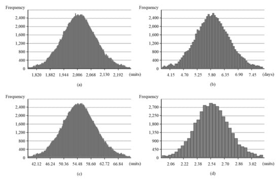
Figure 10.
Control ranges of influencing factors: (a) in-situ production quantity; (b) lead-time; (c) number of molds; (d) number of cranes.
As a result of deriving the Min–Max range of Figure 10c, the number of molds was set to Min 37 units and Max 70 units. Column type 1 is Min 11 and Max 20, column type 2 is Min 5 and Max 10, beam type 1 is Min 2 and Max 7, beam type 2 is Min 16 and Max 26, and beam Type 3 is 3 Min and 7 Max. The reason that the number of individual molds does not decrease below a certain number is that if the number of molds decreases, the timely completion of the in-situ production is impossible. In Figure 10d, as a result of deriving the Min-Max range of the crane, Min was set to two units and Max was set to four units. The number of cranes is the result of calculating the in-situ production cost by rounding up the decimal point of the value derived by the simulation. If a crane is added during construction, it is advantageous to shorten the construction time, but this did not increase above a certain level because the cost and CO2 emissions increase. Since the crane was partially added during construction, the number after the decimal point was derived.
In Figure 11, as a result of deriving the management range of in-situ production cost, Min was set to 615 USD and Max was set to 775 USD. In the case of CO2 emission reduction, Min was set to 4557 t-CO2 and Max was set to 5622 t-CO2. That is, it is possible to save more than 14.38%. These values are the results derived for Min 1757 members and Max 2256 members. As a result of analyzing the management scope as described above, the cost and CO2 emissions according to the fluctuations of each factor are generally proportional to each other; thus, a graph of similar shape was found. Using simulation, project participants can predict the management range for in-situ production volume, number of molds, lead-time, and number of cranes under various conditions. In addition, the management scope can be changed according to the site conditions.
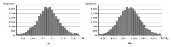
Figure 11.
Control range of cost and CO2 emissions: (a) in-situ production cost; (b) CO2 emission reduction.
5.3. Optimization for Estimating In-Situ Production Quantity
The optimal case is derived by utilizing each management range, such as in-situ production volume, lead-time, mold number, and crane number, which were derived through the Monte Carlo simulation. Lim et al. explained six assumptions about the available area, which is selected as the main influencing factor, and derived the highest cost reduction rate among the scenarios applicable to the case project [20]. However, in this study, factors influencing CO2 emissions are selected and the Min–Max of the influencing factor is derived through simulation. From the derived control range, an optimal value is derived to reduce environmental loads by 10% within a range that can reduce costs by 10% or more.
For simulation, it is assumed that the 18 months required by the client are observed. Table 5 shows the values of the influence factors corresponding to the highest value of the CO2 emission reduction ratio of 14.58%. The quantity is 1,757 members, accounting for 78% of the total quantity, lead-time is 3.8 weeks, number of molds is 37 units, and number of cranes is two units. In-situ production reduced costs by 6,966,000 USD and CO2 emission by 7557 t-CO2 compared to in-plant production. In-situ production costs can be reduced by 10.53% compared to in-plant production. The proposed dynamic optimization model can derive an optimal case in consideration of the CO2 emission reduction ratio and the cost reduction ratio. In addition, it can support decision-making on whether or not in-situ production can be applied to the field.
Table 5.
Optimization result of estimating in-situ production quantity.
5.4. Discussion
The construction industry has the potential to improve productivity by applying prefabrication for building [44]. However, automation and robotics are still not common in the construction field [44,45]. Prefabrication has been plagued by dependence on conventional methods [46], complex interfacing [47], scheduling complexity [48], underutilization of factory space [44], cost barriers [49], fragmented information [50], and inconsistent quality [51].
The in-situ production proceeds in the order of installation of rebar setting, pouring concrete, curing, and stacking [16], and is performed at the same level as in-plant production. After stacking the cured PC members, quality checks and finishing work are done by the manpower if there is partial damage to the surface. In other words, PC members are manufactured at the factory, but the production process is mostly performed by manpower rather than automation or robotics. In the case of in-plant production, there is no actual mechanization except for the use of overhead and gantry cranes in the factory. It was assumed that the idle time of the crane used for erection of PC members is used during in-situ production in this study. In general, although the same sizes of PC columns and beams are designed, the rebar arrangements are not designed with the same PC members. In order for PC members to be manufactured, checked, and installed in the same manner as in the design drawing, work by manpower is required. Therefore, to apply in-situ production in the future, it is required to design PC members with the same size and reinforcement details.
Some of the members that have been produced in-plant have had to be reproduced due to issues with cracks, size, and breakage, as well as rebar arrangements that are different from the drawings. According to an interview with a PC factory official, it was confirmed that if the factory owner does not obtain more than 20% of the production cost as a profit, the official does not contract, because this does not cover the factory management overhead [17]. Through several studies, it has been possible to secure the quality and economic feasibility of in-situ production [14,15,16,17,19]. This study examined in-situ production at a construction site that complied with the PC production and installation guidelines of the KCI (Korea Concrete Institute); it was confirmed that there were no problems with cracks, breakages, size, or strength quality standards.
This study focused only on the factors of in-situ production quantity, lead-time, number of molds, and number of cranes with respect to CO2 emissions. It was assumed that the production time and area were sufficient. However, if various field conditions, such as time and production, are additionally considered, different results will be derived. In-situ production can be applied only to sites where the production area is secured due to concerns about interference with ongoing construction, interference around the site, and safety issues.
In this study, a simulation for in-situ production was performed only for PC columns and beams. This means that slender parts, such as columns and beams, can be produced on-site. PC slabs, such as double-T and rib-plus slabs, occupy a large space during production, so in-plant production is more advantageous than in-situ production [18]. That is, in-plant production can be more advantageous depending on the type and number of members. Long-span and heavily loaded buildings, such as the case project examined in this study, can easily secure a production area due to the long distance between columns. However, different results from this study can be derived depending on the site characteristics and the building size.
6. Conclusions
This paper presented a dynamic optimization model that can dynamically predict, control, monitor, and manage five major influencing factors that affect environmental loads during in-situ production. In order to minimize environmental loads, the in-situ production quantity can be adjusted within the range of fluctuations in influence factors. The effect of the model was verified through the simulation results, and the findings are as follows.
First, the optimization model easily and quickly calculated the range of changes in environmental loads by analyzing the dynamic relationship of influencing factors. According to the simulation of the optimization model, in-situ production can reduce a Min of 4557 t-CO2 and Max of 5622 t-CO2 compared to in-plant production, which resulted in saving more than 14.58%. Second, the optimization model uses simulation results to create the control range of each influence factor to achieve the target environmental load reduction rate within the target cost reduction range. In the case project, the control range of the in-situ production quantity was 1757–2256 members to achieve the target environmental load reduction rate of 10% or more. In other words, project participants can predict the extent to which influencing factors are managed under various conditions. Third, the proposed dynamic model supports decision-making as to whether in-situ production can be applied in the field. The derived optimal case to minimize the environmental loads from the case project resulted in a quantity of 1757 members through the simulation model. In-situ production was able to reduce environmental loads by 14.58% and cost by 10.53% compared to in-plant production. Fourth, material use accounts for more than 61.0% of total CO2 emissions, so its quantity has the greatest effect on CO2 emissions. As the amount of reinforcing bar with a large basic unit of CO2 emissions increases, the environmental loads of the member increase. Overdesign should be avoided.
The model developed in this paper can control the influence factors of in-situ production and can easily and quickly simulate the influences of factors that change during project execution to derive the optimum value according to the situation. When applying in-situ production using this model, environmental loads of CO2 emissions can be calculated at the design stage. Furthermore, it is possible to evaluate whether it is applicable at the initial stage of the project in order to establish and review a construction plan. All these values can be used to analyze economic and environmental feasibility. In addition, they can be used to develop a data management system and build a risk management model for analyzing environmental loads of in-situ production in the future. Further research is needed to calculate the optimal in-situ production quantity considering environmental load through more field applications.
Author Contributions
Conceptualization, J.L.; methodology, J.L.; validation, J.L.; formal analysis, J.L.; investigation, J.L.; data curation, J.L.; writing—original draft preparation, J.L. and J.J.K.; writing—review and editing, J.L. and J.J.K.; visualization, J.L.; supervision, J.J.K.; project administration, J.L and J.J.K.; funding acquisition, J.L. All authors have read and agreed to the published version of the manuscript.
Funding
This work was supported by the National Research Foundation of Korea (NRF) grant funded by the Korea government (MOE) (No. NRF-2019R1A6A3A12032427).
Conflicts of Interest
The authors declare no conflict of interest. The funders had no role in the design of the study; in the collection, analyses, or interpretation of data; in the writing of the manuscript, or in the decision to publish the results.
References
- Intergovernmental Panel on Climate Change (IPCC). Working Group I Contribution to the IPCC Fifth Assessment Report Climate Change 2013; Cambridge University Press: Cambridge, UK, 2013. [Google Scholar]
- Jung, K.O.; Chung, Y.K. The pollution and economic growth based on the multi-country comparative analysis. J. Ind. Econ. Bus. 2004, 17, 1077–1098. [Google Scholar]
- Sartori, I.; Hestnes, A.G. Energy use in the lifecycle of conventional and low energy buildings: A review article. Energy Build. 2007, 39, 249–257. [Google Scholar] [CrossRef]
- Giesekam, J.; Barrett, J.; Taylor, P.; Owen, A. The greenhouse gas emissions and mitigation options for materials used in UK construction. Energy Build. 2014, 78, 202–214. [Google Scholar] [CrossRef]
- Ecoinvent. Ecoinvent Database. Available online: http://www.ecoinvent.org/ (accessed on 1 August 2019).
- Giama, E. Life cycle versus carbon footprint analysis for construction materials. In Energy Performance of Buildings; Springer: Cham, Switzerland, 2016; pp. 95–106. [Google Scholar] [CrossRef]
- Jeong, K.; Hong, T.; Kim, J. Development of a CO2 emission benchmark for achieving the national CO2 emission reduction target by 2030. Energy Build. 2018, 158, 86–90. [Google Scholar] [CrossRef]
- Lee, M.C. Reducing CO2 emissions in the individual hot water circulation piping system. Energy Build. 2014, 84, 475–482. [Google Scholar] [CrossRef]
- Mergos, P.E. Seismic design of reinforced concrete frames for minimum embodied CO2 emissions. Energy Build. 2018, 162, 177–186. [Google Scholar] [CrossRef]
- Lee, J.H.; Kim, K.; Kim, H. Environmental load estimating model of NATM tunnel based on standard quantity of major works in the early design phase. KSCE J. Civ. Eng. 2018, 22, 1040–1051. [Google Scholar] [CrossRef]
- Tae, S.; Shin, S.; Kim, H.; Ha, S.; Lee, J.; Han, S.; Rhee, J. Life cycle environmental loads and economic efficiencies of apartment buildings built with plaster board drywall. Renew. Sustain. Energy Rev. 2011, 15, 4145–4155. [Google Scholar] [CrossRef]
- Priatla, K.; Ariaratnam, S.; Cohen, A. Estimation of CO2 emissions from the life cycle of a potable water pipeline project. J. Manag. Eng. 2012, 28, 22–30. [Google Scholar] [CrossRef]
- Park, J.Y.; Lee, D.E.; Kim, B.S. A study on analysis of the environmental load impact factors in the planning stage for highway project. KSCE J. Civ. Eng. 2016, 20, 2162–2169. [Google Scholar] [CrossRef]
- Hong, W.K.; Lee, G.; Lee, S.; Kim, S. Algorithms for in-situ production layout of composite precast concrete members. Autom. Constr. 2014, 41, 50–59. [Google Scholar] [CrossRef]
- Lim, C. Construction Planning Model for In-situ Production and Installation of Composite Precast Concrete Frame. Ph.D. Thesis, Kyung Hee University, Seoul, Korea, 2016. [Google Scholar]
- Oh, O.J. A Model for Production and Erection Integration Management of Large Scale PC Structures Using System Dynamics. Ph.D. Thesis, Kyung Hee University, Seoul, Korea, 2017. [Google Scholar]
- Lim, J. A Risk Management Model for In-situ Production of Precast Concrete Members Focused on Time and Cost Using System Dynamics. Ph.D. Thesis, Kyung Hee University, Seoul, Korea, 2018. [Google Scholar]
- Lim, J.; Park, K.; Son, S.; Kim, S. Cost reduction effects of in-situ PC production for heavily loaded long-span buildings. J. Asian Archit. Build. Eng. 2020, 19, 242–253. [Google Scholar] [CrossRef]
- Lim, J.; Kim, S. Evaluation of CO2 emission reduction effect using in-situ production of precast concrete components. J. Asian Archit. Build. Eng. 2020, 19, 176–186. [Google Scholar] [CrossRef]
- Lim, J.; Kim, S.; Kim, J.J. Dynamic simulation model for estimating in-situ production quantity of PC members. Int. J. Civ. Eng. 2020, 18, 935–950. [Google Scholar] [CrossRef]
- Na, Y.J.; Kim, S.K. A process for the efficient in-situ production of precast concrete members. J. Reg. Assoc. Archit. Inst. Korea 2017, 19, 153–161. [Google Scholar]
- Lee, G.J. A Study of In-situ Production Management Model of Composite Precast Concrete Members. Ph.D. Thesis, Kyung Hee University, Seoul, Korea, 2012. [Google Scholar]
- Park, S.H.; Lim, C.Y.; Lee, W.J.; Kim, D.S.; Jung, Y.S. The experimental study on concrete manufacturing technologies for ultra high strength concrete pile. In Proceeding of the 2013 Spring Annual Conference of the Korea Concrete Institute, Seoul, Korea, 8–10 May 2013; Volume 25, pp. 67–68. [Google Scholar]
- Won, I.; Na, Y.; Kim, J.T.; Kim, S. Energy-efficient algorithms of the steam curing for the in situ production of precast concrete members. Energy Build. 2013, 64, 275–284. [Google Scholar] [CrossRef]
- Kim, S.; Hong, W.K.; Kim, J.H.; Kim, J.T. The development of modularized construction of enhanced precast composite structural systems (Smart Green frame) and its embedded energy efficiency. Energy Build. 2013, 66, 16–21. [Google Scholar] [CrossRef]
- Dong, Y.H.; Jaillon, L.; Chu, P.; Poon, C.S. Comparing carbon emissions of precast and cast-in-situ construction methods—A case study of high-rise private building. Constr. Build. Mater. 2015, 99, 39–53. [Google Scholar] [CrossRef]
- Yepes, V.; Martí, J.V.; García-Segura, T. Cost and CO2 emission optimization of precast–prestressed concrete U-beam road bridges by a hybrid glowworm swarm algorithm. Autom. Constr. 2015, 49, 123–134. [Google Scholar] [CrossRef]
- Kim, T.; Chae, C.U. Evaluation analysis of the CO2 emission and absorption life cycle for precast concrete in Korea. Sustainability 2016, 8, 663. [Google Scholar] [CrossRef]
- Tan, B.; Huat, D.C.K.; Messner, J.I.; Horman, M.J. Using simulation for pull-driven scheduling with buffer for precast concrete component fabrication and erection. In Proceedings of the 16th CIB World Building Congress, Rotterdam, The Netherlands, 1–7 May 2004; pp. 10–21. [Google Scholar]
- Ballard, G.; Harper, N.; Zabelle, T. Learning to see work flow: An application of lean concepts to precast concrete fabrication. Eng. Constr. Archit. Manag. 2003, 10, 6–14. [Google Scholar] [CrossRef]
- Cho, G.H.; Kim, J.J. Integrated management of the production, transportation and installation of precast concrete panels. J. Archit. Inst. Korea 1996, 12, 185–193. [Google Scholar]
- Karnopp, D.C.; Margolis, D.L.; Rosenberg, R.C. System Dynamics: Modeling, Simulation, and Control of Mechatronic Systems, 5th ed.; John Wiley & Sons: New Jersey, NJ, USA, 2012; ISBN 9781118160077. [Google Scholar]
- Kim, D.; Moon, T.; Kim, D. Chap. System Dynamics, 1st ed.; Daeyoung Book: Seoul, Korea, 1999; ISBN 9788976440600. [Google Scholar]
- Forrester, J.W. Lessons from system dynamics modeling. Syst. Dyn. Rev. 1987, 3, 136–149. [Google Scholar] [CrossRef]
- Kim, I. Risk Management in the Construction Projects, 1st ed.; Kimoondang: Seoul, Korea, 2001; ISBN 9788970864235. [Google Scholar]
- Maio, C.; Schexnayder, C.; Knitson, K.; Weber, S. Probability distribution function for construction simulation. J. Constr. Eng. Manag. 2000, 126, 285–292. [Google Scholar] [CrossRef]
- Korea Institute of Construction Technology (KICT). The Environmental Load Unit Composition and Program Development for LCA of Building, The Second Annual Report of the Construction Technology R&D Program. 2004. Available online: http://www.ndsl.kr/ndsl/search/detail/report/reportSearchResultDetail.do?cn=TRKO201000018952 (accessed on 20 May 2019).
- Hong, W.K.; Kim, J.M.; Park, S.C.; Lee, S.G.; Kim, S.I.; Yoon, K.J.; Kim, H.C.; Kim, J.T. A new apartment construction technology with effective CO2 emission reduction capabilities with effective CO2 emission reduction capabilities. Energy 2009, 35, 2639–2646. [Google Scholar] [CrossRef]
- Hong, W.K.; Park, S.C.; Kim, M.M.; Kim, S.I.; Lee, S.G.; Yun, D.Y.; Yoon, T.H.; Ryoo, B.Y. Development of structural composite hybrid systems and their application with regard to the reduction of CO2 emissions. Indoor Built Environ. 2010, 19, 151–162. [Google Scholar] [CrossRef]
- Lee, D.; Lim, C.; Kim, S. CO2 emission reduction effects of an innovative composite precast concrete structure applied to heavy loaded and long span buildings. Energy Build. 2016, 126, 36–43. [Google Scholar] [CrossRef]
- Lee, S.H.; Joo, J.K.; Kim, J.T.; Kim, S.K. An analysis of the CO2 reduction effect of a column-beam structure using composite precast concrete members. Indoor Built Environ. 2012, 21, 150–162. [Google Scholar] [CrossRef]
- Lim, C.; Lee, S.; Kim, S. Embodied Energy and CO2 emission reduction of a column-beam structure with enhanced composite precast concrete members. J. Asian Archit. Build. Eng. 2015, 14, 593–600. [Google Scholar] [CrossRef]
- Lee, K.; Son, S.; Kim, D.; Kim, S. A dynamic simulation model for economic feasibility of apartment development projects. Int. J. Strateg. Prop. Manag. 2019, 23, 305–316. [Google Scholar] [CrossRef]
- Pan, M.; Pan, W. Determinants of adoption of robotics in precast concrete production for buildings. J. Manag. Eng. 2019, 35. [Google Scholar] [CrossRef]
- Pan, M.; Pan, W. Advancing formwork systems for the production of precast concrete building elements: From manual to robotic. In Proceedings of the 2016 Modular and Offsite Construction (MOC) Summit, Banniff, AB, Canada, 29 September–1 October 2016; pp. 2–9. [Google Scholar]
- Mao, C.; Shen, Q.; Pan, W.; Ye, K. Major barriers to off-site construction: The developer’s perspective in China. J. Manag. Eng. 2015, 31. [Google Scholar] [CrossRef]
- Pan, W.; Gibb, A.G.F.; Dainty, A.R.J. Strategies for integrating the use of off-site production technologies in house building. J. Constr. Eng. Manag. 2012, 138, 1331–1340. [Google Scholar] [CrossRef]
- Arashpour, M.; Wakefield, R.; Abbasi, B.; Lee, E.W.M.; Minas, J. Off-site construction optimization: Sequencing multiple job classes with time constraints. Autom. Constr. 2016, 71, 262–270. [Google Scholar] [CrossRef]
- Pan, M.; Linner, T.; Pan, W.; Cheng, H.; Bock, T. A framework of indicators for assessing construction automation and robotics in the sustainability context. J. Clean. Prod. 2018, 182, 82–95. [Google Scholar] [CrossRef]
- Li, X.; Shen, G.Q.; Wu, P.; Fan, H.; Wu, H.; Teng, Y. RBL-PHP: Simulation of lean construction and information technologies for prefabrication housing production. J. Manag. Eng. 2018, 34. [Google Scholar] [CrossRef]
- Hwang, B.G.; Shan, M.; Looi, K.Y. Key constraints and mitigation strategies for prefabricated prefinished volumetric construction. J. Clean. Prod. 2018, 183, 183–193. [Google Scholar] [CrossRef]


© 2020 by the authors. Licensee MDPI, Basel, Switzerland. This article is an open access article distributed under the terms and conditions of the Creative Commons Attribution (CC BY) license (http://creativecommons.org/licenses/by/4.0/).