Modelling as a Tool for the Planning of the Transport System Performance in the Conditions of a Raw Material Mining

Abstract

This article is devoted to modelling of the extracted raw material removal from a mining area to the entry point for the next technological process. Two approaches were chosen for the process modelling. The first approach is regarded to traffic modelling by using available mathematical equations, based on capacity conversion and calculation of loading equipment efficiency. The second approach of modelling is computer simulation within the simulation system ExtendSim8. The modelling of the transport system and the determination of its efficiency were performed at the same conditions. The examined transport system was consisted of two lorries and one loader. The article presents the results of calculations and the results of simulation experiments, which also verified the results obtained by calculations. Calculations of the transport system performance and simulation experiments were performed for two time periods, for a time of 1 h and 6 h during a shift from three different loading places, which were 500, 1100 and 1450 m away from a place of unloading. The results obtained by both approaches are comparable. The main contribution, novelty, of this article is the modelling of the process in a quarry operation (loading and removal of mineral resources) not only on the basis of available mathematical formulas but also the application of simulation in the simulation tool EXTENDSim8, performing simulation experiments for specified conditions and their comparison with calculated values. Simulation is a suitable tool for determining and subsequently planning of the performance of both existing and projected transport systems.

1. Introduction

The essence of sustainable development is the efficient use of natural resources [1]. The mining and processing industry of raw materials contributes to a huge share in the national economy and delivers an invaluable resource for modern civilization [2].

Transport is the movement of goods over a certain distance or a change in the position of goods by means of transport. Technological processes in the mining industry include various raw material transportation operations which consume significant amounts of energy and generate a substantial share of overall mining costs [3]. In addition to excavation, mining, processing and shipping, transport is the most important service process in both deep and surface mines. Great attention is paid to transport in the extraction and processing of raw materials, because it cannot technically lag behind the mining technique and finally not to become as a brake on the entire technological process of mining [4]. The main task and goal of transport is to ensure the loading, unloading and transfer of the required amount of raw material from a place of extraction to a place of its further processing in the required amount, on time and with minimal costs [5]. In terms of the method of raw materials mining minerals, it is possible to identify two groups of transport systems: transport systems of raw materials in deep mining and transport systems of raw materials in surface mining. Existing transport methods that are feasible for deep mines include lorry transport, shaft systems, and belt conveyors [6,7]. Regarding the surface mining, it is the most common mining method worldwide, and open pit mining accounts for highest surface output. Open pit mining consists primarily of the removal of topsoil and overburden, drilling and blasting of ore, and the transportation of material uses a system of excavators or conveyors and dump trucks [8].

The amended Act no. 51/1988 Coll. of Law of the Slovak National Council on Mining Activities, Explosives and the State Mining Administration, effective from 1 September 2019, is valid for mining activities in the Slovak Republic. All mining activities must meet the requirements in terms of safety, health at work and reliability of operation set by Act no. 124/2006 Coll. of Law on the safety and health protection at work and on amendments to certain acts as amended and Decree (21/1989 Coll.) of the Slovak Mining Authority (from 29 December 1988) about the safety and health protection at work and operational safety in mining activities and activities performed mining underground in Slovakia.

The subject of research in this article is the transport of raw materials in a quarry. Various cyclic and continuous systems or their combinations are used for disposition of disjointed rocks in quarry operations, depending on operating conditions. While in the surface coal mines, long-distance belt conveyors are used on a large scale for the transport of coal [9], the most frequently used transport in quarries is by a lorry. Problems related to this area of transport are solved by several authors, the problems focused on e.g., selection of open-pit dump trucks during quarry reconstruction [10], a procedure to select loading and transportation machines for an open pit complex [11], the procedures are proposed to obtain an optimized number of trucks and to estimate the maximum mining capacity [12], problems to determine the optimal haulage routes of trucks in large scale open-pit mines multi-criteria evaluation [13], application of optimization in Open Pit Mining [14], safety problems [15], environmental impacts, e.g., a proposes a new technology of container carriage of rocks without construction of transport communications in an open-pit mine and with technological and energy-saving advantages [16], to improve the ecological safety of a pit transport [17] and other.

Operation of the transport system, selection of suitable means of transport, their compliance with the loading equipment have an impact on the evaluation of the transport system performance but also of the whole company [18,19].

The transport performance is the amount of material that the transport system can transport per time unit must correspond to the amount of material that needs to be removed from a quarry in a certain time for the needs of the next technological process. Fulfilment of the transport performance depends on specific mining conditions, amount of material on a dump, on the performance of used loading equipment and means of transport, on the transported distance, on the organization of work, on the length of the work shift and other conditions [20].

The main goal of the article is to model the transport system by a lorry, in order to determine its performance.

Modelling as a tool for planning of the transport system performance has been used for raw material extraction conditions. It is transformation of the transport system into a digital form, the application of a modern simulation tool, which should be a replacement for the classical approach (conventional calculations). This can be considered as a trial to create such a suitable tool e.g., for raw material extraction and removal planners. A planner can verify the functioning of real operation when changing the system parameters with the model situation (car failure, reduced loader power, idle times due to bad weather conditions, etc.). Modelling and models are applied in different forms and used in different areas of research. The research of modelling or a model creation is dealt with several authors in various areas of research, e.g., modelling of technological processes [21], transport, handling [22,23], logistics, economic, etc. Authors use and present various types of models - mathematical, graphical, simulation, heuristic, etc. Mathematical and graphic models are presented by authors e.g., Šaderová and Bindzár (mathematical and graphical models of loading and unloading process of mining output at a quarry) [24], Marasová (for the transport of backfill material) [22], Straka et al. (the graphic model of unloading with transport of unloaded mineral resources) [25]. Malindžák et al. present the heuristic model for production scheduling wide-strip rolling mill [26]. Petri nets were used for modelling of complex urban traffic networks by authors Flores-Geronimo et al. [27], for modelling interactions among various components as well as the subsystems of a plywood manufacturing plant by authors Kumar et al. [28], for solving problems related to resource planning in intermodal freight transport terminals by authors Cavone et al. [29], for modelling a process of chemical production by authors Trebuna et al. [30]. Currently, the simulation models are relatively widely used, by which authors use to solve mainly problems related to transport, handling, production, logistics and ecology [31,32,33]. Nowadays, several simulation tools are used for computer simulation such as Witness [34], Tecnomatix Plan Simulation [35,36], Extend [37,38], FlexSim [39] Arena [31,40] SimMin [6], MATLAB [33] and others.

Computer simulation has increased its popularity since the 1960s, in the mining industry. During the 1960s, many mining simulations were built by using a computer language called Fortran, subsequently, computer simulations such as the General Purpose Simulation System (GPSS), SIMBELT4, Monte Carlo simulation, a Method of IntegratedProcess Simulation [41] were used, in recent years, it has been SimEvents [42], MATLAB/Simulink [33], ARENA [40].

Based on the findings, the simulation tool EXTENDSim8 has not been utilized in the mining industry, the simulation approach in this article has not been used so far. It is possible to state, based on a short literature review, that the simulation tool chosen by the authors is most often used to model material flows in various areas, but not in the process of a quarry operation.

The main contribution of this article is the modelling of the process in the quarry operation (loading and removal of mineral resources) not only on the basis of available mathematical formulas but also the application of the simulation tool EXTENDSim8 (creation of a functional model), performing simulation experiments for specified conditions and their comparison with calculated values.

The main conclusion of the paper is to prove that the application of the simulation tool EXTENDSim8 is applicable in the conditions of the mining industry. However, any experiments are expensive and time consuming on a real system. The simulation can be performed without affecting the real operation.

Modelling of the removal of extracted raw material from a mining area to an entry point for the next technological process is performed by two approaches. The first approach presents traffic modelling by using available mathematical equations. The second approach of modelling is computer simulation in the simulation system ExtendSim8. Modelling in both approaches will be performed for the same conditions, which are based on real operation and conclusions will be drawn from their results. Other application possibilities of modelling in this case are: What type and number of transport equipment should be used? What is the throughput of the given system? Where are the bottlenecks? How many hours does it take to complete the planned tasks? What percentage of loading and transport vehicles are used?

This paper is processed by a sequence of the following steps: Workmanship of a methodology for determining of transport performance; Defining model conditions based on parameters obtained from selected quarry operation; Determination of the traffic performance of the system based on the capacity calculation of traffic in the quarry; Determination of traffic performance by simulation (creation of the simulation model, model verification, experiments, analysis of the results obtained from simulation experiments); Results discussion and Conclusion.

2. Materials and Methods

The transport system ensures the removal of bulk substrate from the place of extraction. Bulk substrate is a type of mineral raw material (quarry stone) with characteristic properties (physical and chemical), obtained by primary eventually by secondary blasting of the rock mass in a quarry, which can be in several places-levels. A loading (servicing) device loads the substrate and lorries ensure its removal. These lorries are returned to the same loading device after unloading of the substrate at an unloading point. The number of vehicles operating in the system is known in advance. It is a closed queuing system. The diagram of the system with one loading point is shown in Figure 1.

As it was mentioned in the introduction, two approaches were used to plan the performance of this type of transport system. The first approach—mathematical modelling based on available mathematical equations. The second approach—modelling by applying simulation in a selected simulation tool.

2.1. Modelling by Using Mathematical Equations

The basis for modelling of the above mentioned processes is the capacity calculation of road transport and the calculation of the loading equipment performance. The capacity recalculation of road transport consists of calculation of the following parameters [24]:

(A).

The hourly performance of a quarry lorry;

(B).

The number of lorry rounds per hour along a given route;

(C).

The number of lorries needed to handle the loader’s performance.

(A)

The calculation of the hourly performance of one lorry was done by the following Formula (1):

$$P_V=C·\frac{60}{Tc}$$

(1)

where: C—capacity of a lorry [t], Tc—time of one transport cycle (round) [min].

The vehicle turnaround time or the transport cycle time (this term will be used later) from the point of the transport system modelling in a quarry is very important parameter, if not the most important. The term of lorry turnover is an integral part composed of repeated journeys in a certain period of time (shift, day, etc.), which includes loading, driving to a destination, unloading and driving back to a place of loading. Based on this concept, the parameter transport cycle time Tc is given by the sum of loading time t₁, travel time t₂ (travel time with load and travel time without load), unloading time t₃ and possibly lost time or idle time (vehicle waiting, obstacles on the road, etc.) t₄:

$$Tc=t_1+t_2+t_3+t_4$$

(2)

The calculation of the loading time according to the following Formula (3):

$$t_1=\frac{C}{P_{L_E}}·60$$

(3)

where: $P_{L_E}$ is effective hourly loader performance in [t·h⁻¹].

The time of unloading the material from the body of a lorry (backwards or sideways) is given in the manufacturers’ brochures (for example Mining Track BELAZ 75600, the producer declare in its prospect: OPERATIONS TIME: Body raise time 31 s and Body lower time 20 s [43]), it depends on the body tilt control mechanism or time observation in operation, which is in the range from 60 to 90 s.

The lost time depends on the degree of work organization and should be close to zero. A lorry travel time for one transport cycle is calculated as the ratio of the transport distance and the average speed of a lorry. The duration of the transport cycle Tc in specific operating conditions is also determined by time observation.

The time of loading and other non-transport operations is constant for the certain operation and the selected type of lorries and the driving time increases linearly with the transport distance. Thus, if traffic performance is to be kept when the traffic distance is increased, it is necessary to either increase the capacity of a lorry or the number of lorries in proportion to the increasing distance.

The Tc parameter is one of the basic parameters that affect the performance of the transport system.

The performance of the transport system in a certain time period T in hours (shift, day, week, month or year), in which several means of transport provide transport, is calculated as the sum of their performance $P_{V_i}$ multiplied by the duration of the time period T and time utilization coefficient η:

$$P_{TS}=T·\eta ·\sum _{i=1}^n{P}_{V_i}$$

(4)

(B)

The number of lorry turns per hour for a given transport distance—the route is calculated as:

$$N_t=\frac{60}{Tc}$$

(5)

(C)

The number of lorries needed to handle its performance is calculated by the ratio of the effective performance of a loader $P_{L_E}$ and the performance of a lorry $P_V$:

$$N_V=\frac{P_{L_E}}{P_v}$$

(6)

The parameter $P_{L_E}$—effective hourly performance of a loader enters the relations (3) and (6). The effective hourly performance of a loader is determined by calculation based on the Formula (7) [24]:

$$P_{L_E}=\frac{3600}{t_{cl}}·v_b·\rho ·c_f·\eta$$

(7)

where: v_b—loader bucket volume [m³], ρ—bulk density of a raw material [t.m⁻³], c_f—bucket filling coefficient, η—time utilization coefficient, $t_{cl}$—loader working cycle time [s].

The working cycle time of a loader $t_{cl}$, in relation to this formula, can be obtained in two ways: from the technical documentation of an equipment (which often does not correspond to the operating conditions), or directly from the time observation in operation. Time observation is made for a loader work cycle or for particular work cycle operations: time to pick up raw material into a loader bucket, time to lift and turn over full bucket over a vehicle, emptying raw material from a bucket into a vehicle body, time to turn over a bucket and preparation for next bucket filling and lost times.

2.2. Modelling by Applying Simulation

Simulation is the method in which a real system is replaced by a computer model. The created model is set in motion and monitored its behavior in various situations during the simulation run. It is possible to perform a number of experiments with the simulation model, evaluate them and apply the results to a real system. The output of the simulation model can be used to verify the results, which can be obtained by calculation according to known mathematical formulas or by observations directly in operation [38].

The simulation of the transport of a lorry turnaround cycle consists of several steps. The basic steps are described in the following points and shown in Figure 2.

A.

Identification of the system and its graphical interpretation for the needs of a simulation model creation. In this step, the real transport system, elements of the system, its surroundings and basic characteristics of the system are identified. A graphical representation of the system is created.

B.

Creating a simulation model by the selected simulation tool. Currently, simulation packages are used for creating a simulation, which facilitate the work of creating a model. Their advantage is graphic symbolism, creation of statistics, 2D or 3D animation and flexibility both when changing the model itself and changing the input data.

C.

Simulation of experiments, in which the input parameters of the simulation model are changed. The task of the experiments is to see changes in the output parameters of the system.

D.

Analysis of simulation results and recommendations. Outputs from individual experiments (statistical parameters, performance parameters and graphical outputs) are used for analysis and behavior of the system under changed conditions. These results need to be interpreted and used correctly.

The results obtained from the simulation can be applied to a real system and can be used as an assessment of the current state of the system, finding a bottleneck in the system, etc. The advantage of the simulation is also at the visual side—display of both the system and the results obtained from experiments. A simulation also has its disadvantages and its application is also associated with some problems. One of disadvantages is the requirement for quality and relevant data, it is not possible to test the correctness of the function of the compiled model without them. Other disadvantages include: the construction of the model requires a perfect knowledge of the modelled object, the process but also the simulation environment itself, the level of detailed modelling depends on this knowledge; quantitative parameters are not standard (it is necessary to change the parameters in the model when changing the vehicle, loader, etc.); the obtained results are interpreted only for the purposes for which the model was formulated; it does not guarantee the acquisition of optimal values of the investigated system parameters; if the simulation model is reused, it is necessary to ensure its constant updating to changes that occur in the real system.

ExtendSim8 simulation tool was used in this study, which is based on discrete event simulation principles. This simulation tool is one of the open source simulation tools (possibility to rework and modify blocks according to the user’s needs), with the so-called “drag and drop” support. This unique simulation tool was not chosen by a chance. The given simulation tool, available to the authors, is used not only to support research but also as an innovative teaching support for the development of competencies in the field of logistics. ExtendSim8 allows simulation of a chosen system or process by creating its logical structure in an easy-to-use format, based on the authors’ previous experience. It has user-friendly interface, which is really good and easy to use.

3. Results

3.1. The Model Conditions

Modelling of the transport system performance was provided for these model conditions: for a loading device (a hydraulic excavator on a crawler chassis and the bucket volume of 2.5 m³), which is used to load a quarry stone in a quarry after blasting; and for a lorry with a load capacity of 15.2 tons (8 m³), which is used to transport a quarry stone. This loader must perform 3 work cycles to load one lorry, (it represents 13.2 tons, the capacity of a lorry is used to 87% and the volume of the body is used up to 94%) [44]. There are 3 loading places (floors) in a quarry, located at different distances from the unloading place. The loading of a quarry stone is provided at the given time from only one place in operation. The mentioned loader does not move among loading positions during the working shift. The specific place of stone loading depends on the mining process in a quarry. The basic operating parameters entering into the calculations are in

Table 1. Entering parameters for the process modelling.

Parameter	Value
Bulk density of a material, ρ [t·m−3]	1.8
Bucket filling coefficient, cf [-]	0.8
Excavator bucket volume, $v_b$ [m3]	2.5
Weight of material in the excavator bucket, [t]	4.4
Loader working cycle time, $t_{cl}$ [seconds]	48
A quarry lorry capacity, C [t]	13.2
Number of lorries in operation, [pcs]	2
Shift length, T [hours]	8
Time utilization coefficient per shift, η [-]	0.75
Raw material unloading time, t3 [seconds]	43
Place of loading	P1	P2	P3
Transport distance among the places of loading and unloading, D [km]	0.5	1.1	1.45
Average speed of a lorry with/without load, [km/h]	6/9	9/12	9/12

.

3.2. Capacity Calculation of Road Transport and Determination of the Transport Performance

The parameter t_cl—loader working cycle time was determined into relation (7) on the basis of time observation of the loader working cycle at the loading site. The basic working operations of the loader working cycle were measured: the time of loading the raw material into the bucket, the driving time with the full bucket, the emptying of the raw material from the bucket on the lorry body, the driving time with the empty bucket back to the preparation for next loading and lost times. The arithmetic mean of the measured values of the loader working cycle (48 s) was added into Equation (7). The effective hourly performance of the loader represents 1.640 tonnes of raw material per shift, calculated according to Formula (7)—$P_{L_E}$ = 205 tonnes per hour.

Table 2. Input data and calculation results for each loading position.

Place of Loading	Transport Distance [km]	Driving Time with the Load [min]	Driving Time without the Load [min]	Tc [min]	${\mathit{P}}_{\mathit{V}}$ [t/h]	${\mathit{N}}_{\mathit{t}}$ [pcs]	${\mathit{N}}_{\mathit{V}}$ [pcs]	${\mathit{P}}_{\mathit{T}\mathit{S}}$ [t/shift]
P1	0.5	5	3.34	13.92	56.9	4.3	3.6	682.92
P2	1.1	7.34	5.5	18.42	43	3.3	4.7	516.05
P3	1.45	9.67	7.25	22.5	35.2	2.66	5.8	422.40

involves the calculated values: driving time with the load, driving time without the load, traffic cycle time according to Formula (2), hourly lorry performance according to Formula (1), system traffic performance per shift according to Formula (4), number of lorry rounds per hour according to Formula (5) and the number of lorries needed to handle the loader performance according to Formula (6), the loading time being calculated according to Formula (3) t₁ = 3.9 min. Unloading time was determined to t₃ = 43 s by operation. This time includes bringing the vehicle to be unloaded, lifting the lorry body and emptying the raw material, lowering the lorry body to the transport position. Lost times were determined by estimating t₄ = 1 min.

Table 2 also shows that the performance of the transport system represents, at the best case, only 42% of the loader performance for the loading site P1 (31% for P2 and 26% for P3). This fact is also confirmed by the parameter N_V. It can be stated that the given transport system has reserves for increasing its performance based on the calculation.

3.3. Simulation

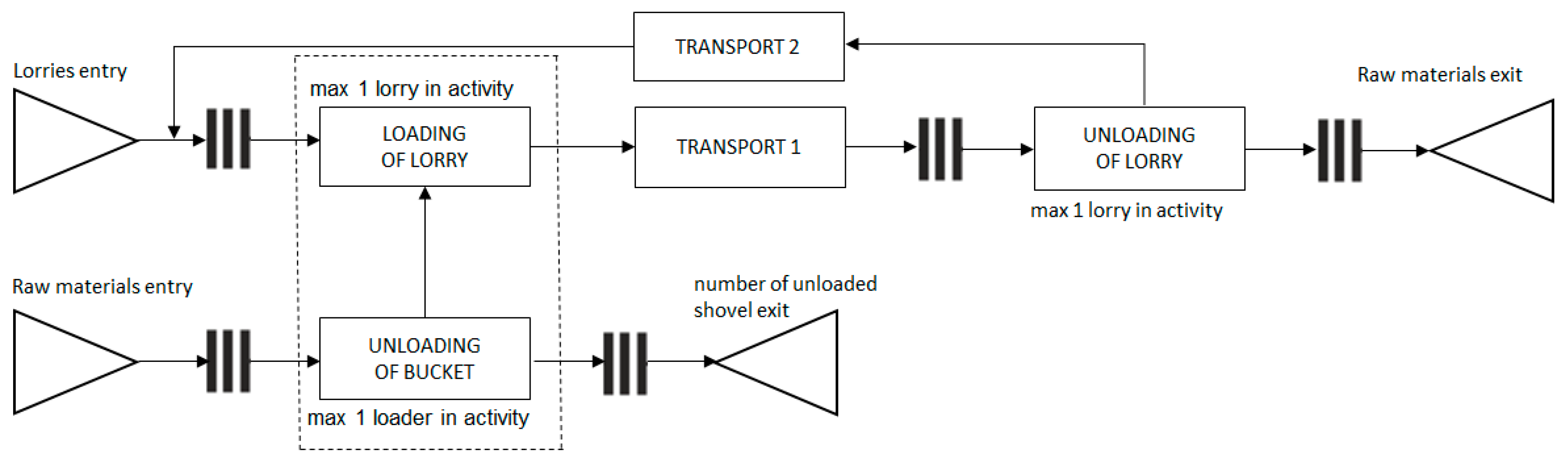
3.3.1. The Simulation Model

As it was stated above, the simulation model was created in ExtendSim8. The simulation model is created by blocks that are connected with junctions, which determine the direction of the flows (flow of raw materials, flow of lorries). Each used block represents the part of the process or operation in the simulation model. The blocks have its unique icon and name there expresses its basic usage within the model [45]. The created simulation model is the model of discrete simulation created from blocks taken from the “Discreet Event” and “Plotter” libraries.

The model is made up of two parts as it can be seen from Figure 3. The first part of the model represents the lorry rides. The second part of the model represents the work of the loader.

The first entry into the model represents requirements (lorries). The “Create1-Lorries” block was used to generate inputs, the number of generated requirements (lorries) entering the system is set in this block.

The block “Queue1” represents the queue of requirements (lorries waiting for loading).

The block “Gate1” provides control of the lorry loading. This block will ensure the delay of next lorry for the loading process, it will not allow its loading while previous lorry is being loaded. If the loading of the lorry is completed, the block will release next lorry for loading.

The block “Activity—Loading of Lorry” represents the loading of raw materials into the lorry.

“Gate 2”—block provides a check whether the lorry is already fully loaded. If the lorry is not yet full, then the “Gate 2” block will not let it go to the next operation (Transport). If the lorry is fully loaded, then the “Gate 2” block will let the lorry leave the activity loading. The “Gate2” block is informed of the fully loaded lorry via the “Decision” block provided the condition be met that is the given lorry maintained at least “A” pcs of loading buckets, what represents a discharge of one full lorry to next activity.

The block “Transport 1” is a journey that the lorry has to take from a place of loading to a place of unloading. The time is set in this block, which represents the driving time.

The block “Queue2” represents a series of requests (lorries waiting to be unloaded).

The block “Activity—Unloading of Lorry” represents unloading of raw materials from the lorry. The time that represents the unloading of raw materials from the lorry is set in this block.

The block “Transport 2” is the journey back that the lorry has to go from a place of unloading to a place of loading of raw materials. The time is set in this block, which represents the reverse travel time.

The block “Select Item In” is intended to ensure that returning lorries are get back to a queue for re-loading.

The second input to the model represents the requirements (batches of a raw material, which are loaded into the lorry by one loader bucket, equal to the volume/load capacity of the loader bucket). The block “Create2-Raw material” block was used to generate inputs. The number of generated requests (batches of a raw material) that enter the system is set in this block.

The block “Queue3” represents a series of requirements (batches of a raw material that will be loaded into the lorry).

The block “Gate3” provides control if there is an empty lorry available. If the lorry is available, the block “Gate3” will allow further loading of a raw material into the lorry. If the lorry is not available, then the “Gate3” block prevents the loading of a batch of a raw material.

The block “Activity—Loader duty cycle” block represents one work cycle of the loader, loading one batch of a raw material into the lorry. The time is set in this block, which represents the time of one working cycle of the loader.

The block “Information” indicates information whether the required number of “A” batches of a raw material (buckets) has been loaded to fill one lorry. The block sends this information to the “Holding Tank” block.

The block “Holding Tank” starts the cycle of loading one batch of a raw material into the lorry via the information block.

The block “Decision” compares the number of batches of a raw material with the value “A”, which represents the number of batches of a raw material (full buckets) for filling one lorry. The value of “A” was determined in advance (Section 3.1), based on the parameters of the lorry and the loader bucket.

The block “Math” performs the selected mathematical operation on the inputs and the result is on the output.

The block “Exit” represents the output of the requirements, the number of batches of a raw material that were loaded into the lorry in total.

The block “Discrete Event” draws graphs of the simulation performance from the input values and it writes the values of the monitored inputs to a table.

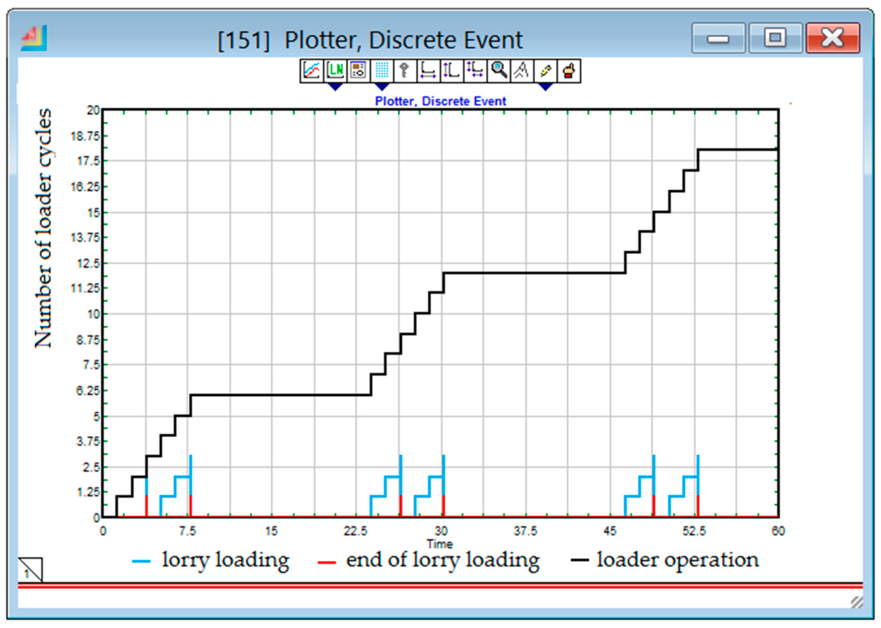
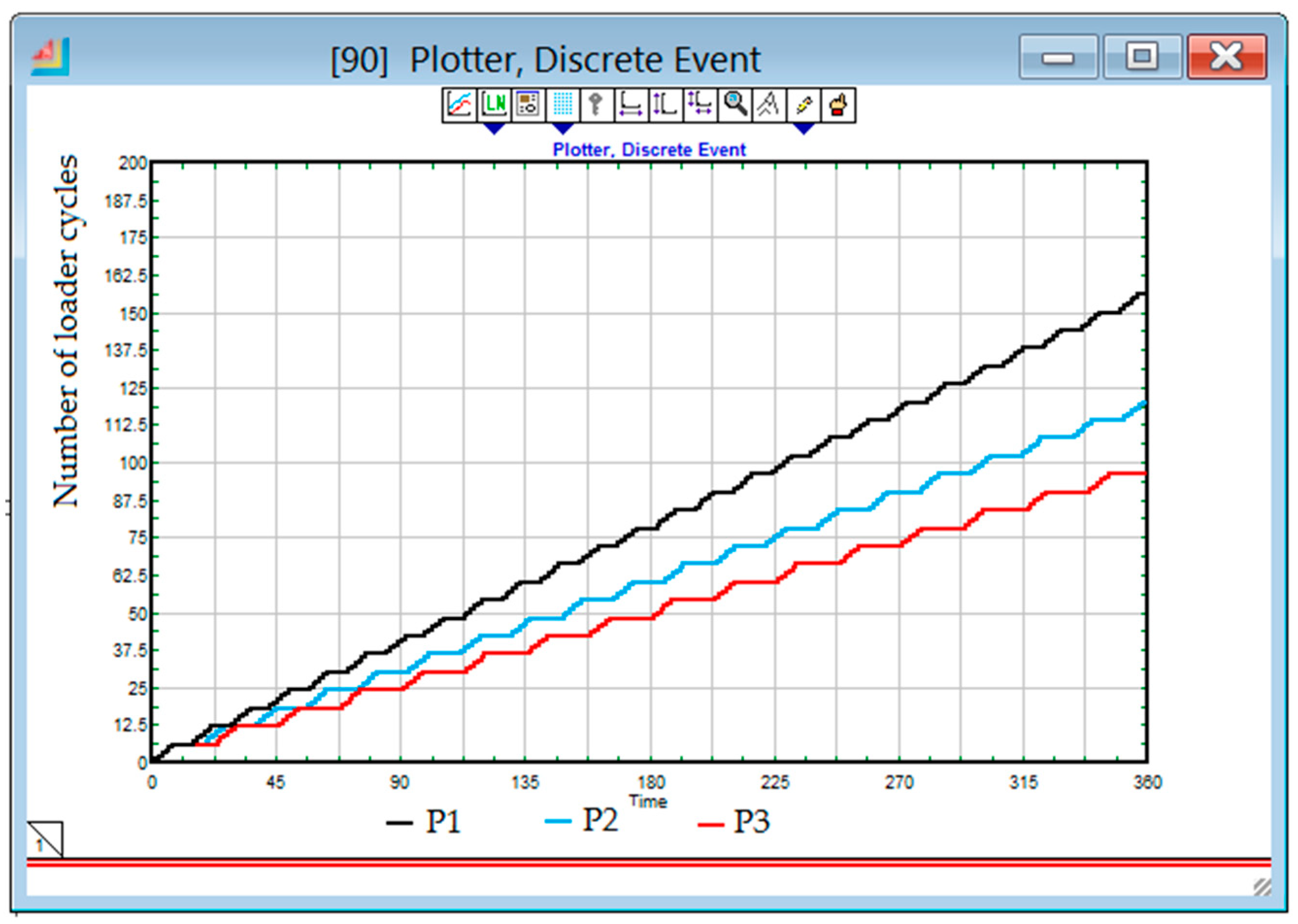
3.3.2. The Simulation Experiments and the Simulation Analysis

Experiments for model conditions were performed on the created simulation model. The setting of block parameters was performed in a similar way as in the article: Proposal for the simulation model of the combined raw materials transport system by authors Straka et al. [45]. The value “A” = 3 was set in the block “Decision”, so that the loader must perform 3 working cycles to load one lorry.

Experiment 1 has simulated the transport system for model conditions from the P1 loading site. During the simulated time of 60 min, the loader performed 27 working cycles. The time utilization of the loader was 59%. The loader loaded 9 lorries, 8 lorries were unloaded and lorries performed a total of 8 full cycles.

Experiment 2 has simulated the transport system for model conditions from the P2 loading site. During the simulated time of 60 min, the loader performed 21 working cycles. The time utilization of the loader was 47%. The rest of the time (53% of the simulated time) was the loader idle. During this simulation time, the loader loaded 7 lorries, 6 lorries were unloaded and they has made 6 turns.

Experiment 3 has simulated the transport system for model conditions from the P3 loading site. During the simulated time of 60 min, the loader performed 18 working cycles. The time utilization of the loader was 39%. The rest of the time (61% of the simulated time) was the loader idle. During this simulation time, the loader loaded 6 lorries, 5 lorries were unloaded and they has made 4 turns. The graphic diagram of loading the lorry at location P3 is shown in Figure 4.

The simulation was performed for a simulated time of 6 h for the above experiments, which represents the netto working time of one shift. The loading process of lorries for all three loading locations is shown in Figure 5. The results obtained from the simulation are in

Table 3. The simulation results for a simulated time of 6 h.

	Experiment 1	Experiment 2	Experiment 3
The number of cycles of a loader	155	120	96
Utilisation of a loader [%]	57	44	35
The number of loaded lorries	51	40	32
The number of unloaded lorries	51	38	32
The number of a lorry cycles	50	38	30
ML [t/shift]	682	528	422.4
$P_{TS}$ [t/shift]	673.2	501.6	396

.

There were 51 lorries loaded and unloaded in the simulated time (i.e., one lorry 26 and another lorry 25 times), a total of only 50 complete rounds were performed, at the end of the simulation, one lorry was still on the way back as it can be seen from Table 3 in the Experiment 1 (Figure 6).

The number of loaded and unloaded lorries in the simulated time is different within the Experiment 2. This is due to the fact that both cars were on the road towards the place of unloading (Figure 7) at the end of the simulation.

Assuming that the weight of a raw material in one bucket is 4.4 tons, it is possible to determine the amount of loaded raw material M_L based on the number of loaded lorries from the simulation results (Table 3). The performance of the transport system $P_{TS}$ can be determined on the basis of the number of lorries that have left the place of unloading (Table 3).

4. Discussion

The performance of the transport system for model conditions was determined by calculation and by application of the simulation. The comparison of the results obtained by both approaches is displayed in

Table 4. The comparison of the transport system performance.

Loading Lace Parameter	P1		P2		P3
	Calculation	Simulation	Calculation	Simulation	Calculation	Simulation
$P_V$ [t/hour]	56.9	35.2	43	26.4	35.2	22
$P_{TS}$ [t/hour]	682.92	673.2	516	501.6	422.4	396

. The comparison of the transport performance per one working shift is shown in Figure 8.

Table 3 and Table 4 and Figure 8 show that the traffic performance values obtained from the simulation are lower compared to the calculated values. This difference is due to the fact that the transport performance results obtained from the simulation has taken into account the number of lorries that were unloaded and left the place of unloading. The transport performance determined by mathematical calculation does not take into account whether the number of lorries, that were loaded in a given time period, was also unloaded. If the M_L values from Table 3 and the $P_{TS}$ traffic performance values from Table 4 obtained by the calculation are compared (the values are bold marked) for the loading sites P1 and P3, they are almost the same. The values are different for place P2, which is due to the form of calculation (1) and (4).

It can be stated that the results obtained from the simulation verified the results obtained by the mathematical calculation. Based on this finding, it can be concluded that the simulation is a suitable tool for determining and subsequently planning the performance of the transport system on the basis of relevant data. The main advantage of the simulation is that it is possible to build a model of a designed or existing system and explore several variants of the transport system quite fast. It is possible to change important variables in the model, which is difficult to change in real conditions. The simulation results can be used to optimize the system, or to determine e.g.,: system bottlenecks, idle time of equipment and other means, determine the limits of the existing system, determine how many vehicles of a given load capacity need to be put into real operation to meet daily capacity for: e.g., finishing mill—how the number of vehicles can be changed depending on the length of material transport track, what kind of vehicle to choose for the loader in terms of its load capacity, etc.

Other experiments were performed on the given simulation model. The example is graphically depicted in Figure 9 where the aim is to determine the number of lorries for each loading site to achieve a transport system performance of 800 tons per shift and 900 tons per shift.

In a similar way, the comparison of system performance, e.g., when loading railway wagons [44], mining rail transport performance [46], vertical transport performance [38]. It can be stated, based on the comparison of system performance values, that the performance achieved in mining practice (consultation directly in operation), whether underground or surface, are different compared to simulated values, in most cases lower, due to difficult operating conditions and unforeseen circumstances.

Nowadays and in the near foreseeable future, a quarry road transport will be the most common method of transport in a surface mining. This is due to many advantages of using trucks, their autonomy and also the use of dispatching control by automated systems, which have the effect of reducing transport costs, which often include most of the costs of surface mining. The economic viability of a modern quarry depends on careful planning and management. The paper gives an example of the transport system performance determining. The results obtained in the paper, also presented in simulation form, suitably not only replace, but also verify the accuracy of the calculated values.

Models in several papers are processed and applicable only for a quarry conditions for which they were solved. It can be stated that the model proposed in this article is applicable for the planning performance in several quarries where this type of transport system is used. The model will provide transport performance results for any loading point and transport route by changing the parameters in the corresponding blocks. The presented model is easily adaptable for different loading points, for increasing and decreasing the number of used lorries. It is also applicable for the situations where it is necessary to obtain system performance by changing the capacity of a loader or a lorry. It means that it is a suitable tool for data acquisition e.g., for multicriteria evaluation of several system variants. This case study confirmed that dynamic simulation can add value and predict planning of the transport system performance.

Company managers should make this change on the basis of data obtained by simulation (verification of several variants of change) and consider their acceptability on the basis of several criteria (functionality, performance or reliability) before the actual implementation of any system change. Simulation of a larger number of system variants can indicate both positive and negative changes after an intervention in a system. The specific steps of implementing a simulation may differ depending on whether simulations are performed directly in-house or outsourced. In case that a company wants to implement simulation itself, the implementation steps would include e.g.,: the selection of a person responsible for the simulation (necessary knowledge of a system), definition of simulation requirements, software selection, purchase of software and hardware, training in software use, first pilot project (model compilation, analysis of results), etc. Company managers will define the requirements for simulation experiments, evaluate the provided data and make decisions based on these data.

5. Conclusions

This article describes to the determination of the transport system performance in a quarry operation. Performance for the model situation was determined by two approaches, mathematically and based on the results obtained from the simulation. The results from these two approaches are comparable. The main parameters that affect the performance of the transport system, in addition to the duration of the transport cycle and the capacity of the vehicle, are also the performance of the loader and its compliance with the vehicle. The correlation between the number and capacity of loading equipment and the number of means of transport working in these systems is one of the most important optimization problems in the transport system. These two parameters are in a conflicting relationship. If there are assigned too many vehicles to the given system, it is not enough to operate a loading (servicing) device in the system of circulating vehicles and queues are formed, while the utilization of vehicles decreases. On the other hand, the lower number of vehicles causes unnecessary idle times of the loading device.

The simulation model is a suitable auxiliary tool for the decision-making process, whether in the design of new systems or the evaluation of existing systems based on the performed experiments.

The simulation of systems can be performed outside of a real object, without affecting the actual operation or without the existence of a real system. The simulation model presented in this article can be applied after modifications to other (similar) technological systems, not only to the transport system in a quarry. It is also possible to extend the model to other activities that future research should be addressed to. The future research will be also focused on creating a simulation model in another simulation tool. Plant Simulation, the standard software for simulation of very complex production systems, is available at the workplace, which can also include transport systems for the extraction and processing of raw materials. The results of experiments performed by created models will be analysed and compared, the advantages and disadvantages of created models will be also determined.

References

1. Behun, M.; Kascak, P.; Hrabcak, M.; Behunova, A.; Knapcikova, L.; Sofranko, M. Investigation of Sustainable Geopolymer Composite Using Automatic Identification Technology. Sustainability 2020, 12, 6377. [Google Scholar] [CrossRef]
2. Sofranko, M.; Khouri, S.; Vegsoova, O.; Kacmary, P.; Mudarri, T.; Koncek, M.; Tyulenev, M.; Simkova, Z. Possibilities of Uranium Deposit Kuriskova Mining and Its Influence on the Energy Potential of Slovakia from Own Resources. Energies 2020, 13, 4209. [Google Scholar] [CrossRef]
3. Krol, R.; Kawalec, W.; Gladysiewicz, L. An Effective Belt Conveyor for Underground Ore Transportation Systems. In Proceedings of the IOP Conference Series: Earth and Environmental Science, Prague, Czech Republic, 11–15 September 2017; Volume 95, pp. 1–10. [Google Scholar] [CrossRef]
4. Sofranko, M.; Listiakova, V.; Zilak, M. Optimizing transport in surface mines, taking into account the quality of extracted raw ore. Acta Montan. Slovaca 2012, 17, 103–110. [Google Scholar]
5. Saderova, J. The selection of loading and transportation means in quarry. In Proceedings of the SGEM 2019 Conference Proceedings, 1.3. Science and Technologies in Geology, Exploration and Mining: Exploration and Mining Mineral Processing, Albena, Bulgaria, 30 June–6 July 2019; STEF92 Technology: Sofia, Bulgaria, 2019; pp. 677–684. [Google Scholar] [CrossRef]
6. Greberg, J.; Salama, A.; Gustafson, A.; Skawina, B. Alternative Process Flow for Underground Mining Operations: Analysis of Conceptual Transport Methods Using Discrete Event Simulation. Minerals 2016, 6, 65. [Google Scholar] [CrossRef] [Green Version]
7. Wolny, S. Emergency braking of a mine hoist in the context of the braking system selection. Arch. Min. Sci. 2017, 62, 45–54. [Google Scholar] [CrossRef] [Green Version]
8. Manyele, S. Analysis of Waste-Rock Transportation Process Performance in an Open-Pit Mine Based on Statistical Analysis of Cycle Times Data. Engineering 2017, 9, 649–679. [Google Scholar] [CrossRef] [Green Version]
9. Marasova, D.; Zolotukhin, V.; Ambrisko, L. Application of the ecological closed transport systems in mining industry. In Proceedings of the SGEM 2019 Conference Proceedings, 1.3. Science and Technologies in Geology, Exploration and Mining: Exploration and Mining Mineral Processing, Albena, Bulgaria, 30 June–6 July 2019; STEF92 Technology: Sofia, Bulgaria, 2019; pp. 57–64. [Google Scholar]
10. Burmistrov, K.V.; Osintsev, N.A.; Shakshakpaev, A.N. Selection of Open-Pit Dump Trucks during Quarry Reconstruction. Procedia Eng. 2017, 206, 1696–1702. [Google Scholar] [CrossRef]
11. Kumykova, T.M.; Kumykov, V.K. Method of Shaping Loading-and-Transportation System in Deep Open Pit Complex Ore Mines. J. Min. Sci. 2017, 53, 708–717. [Google Scholar] [CrossRef]
12. Tan, Y.; Miwa, K.; Chinbat, U.; Takakuwa, S. Operations modeling and analysis of open pit copper mining using GPS tracking data. In Proceedings of the 2012 Winter Simulation Conference (WSC), Berlin, Germany, 9–12 December 2012; pp. 1–12. [Google Scholar] [CrossRef] [Green Version]
13. Yosoon Choi, Y.; Park, H.-D.; Sunwoo, C.; Clarke, K.C. Multi-criteria evaluation and least-cost path analysis for optimal haulage routing of dump trucks in large scale open-pit mines. Int. J. Geogr. Inf. Sci. 2009, 23, 1541–1567. [Google Scholar] [CrossRef]
14. Caccetta, L. Application of Optimisation Techniques in Open Pit Mining. In Handbook of Operations Research in Natural Resources; Weintraub, A., Romero, C., Bjørndal, T., Epstein, R., Miranda, J., Eds.; Springer: Boston, MA, USA, 2007; Volume 99. [Google Scholar] [CrossRef]
15. Abbaspour, H.; Drebenstedt, C.; Dindarloo, S.R. Evaluation of safety and social indexes in the selection of transportation system alternatives (Truck-Shovel and IPCCs) in open pit mines. Saf. Sci. 2018, 108, 1–12. [Google Scholar] [CrossRef]
16. Sergey Kuzmin, S.; Kadnikova, O.; Altynbayeva, G.; Turbit, A.; Khabdullina, Z. Development of a New Environmentally-Friendly Technology for Transportation of Mined Rock in the Opencast Mining. Environ. Clim. Technol. 2020, 24, 341–356. [Google Scholar] [CrossRef]
17. Koptev, V.Y.; Kopteva, A.V. Improving Pit Vehicle Ecology Safety. J. Phys. Conf. Series 2018, 1015, 052014. [Google Scholar] [CrossRef] [Green Version]
18. Kot, S. Cost structure in relation to the size of road transport enterprises. Promet 2015, 27, 387–394. [Google Scholar] [CrossRef] [Green Version]
19. Straka, M.; Rosova, A.; Malindzakova, M.; Khouri, S.; Culkova, K. Evaluating the Waste Incineration Process for Sustainable Development through Modelling, Logistics, and Simulation. Pol. J. Environ. Stud. 2018, 27, 2739–2748. [Google Scholar] [CrossRef]
20. Sofranko, M.; Wittenberger, G.; Skvarekova, E. Optimisation of technological transport in quarries using application software. Int. J. Min. Miner. Eng. 2015, 6, 1–13. [Google Scholar] [CrossRef]
21. Malindzakova, M.; Straka, M.; Rosova, A.; Kanuchova, M.; Trebuna, P. Modeling the process for incineration of municipal waste. Przem. Chem. 2015, 94, 1260–1264. [Google Scholar]
22. Marasova, D. Proposal of alternatives for the transport of backfill material based on the capacity calculation of truck transport in mining conditions: Case study. In Proceedings of the SGEM 2018 Conference Proceedings, 1.3. Science and Technologies in Geology: Exploration and Mining, Albena, Bulgaria, 2–8 July 2018; STEF92 Technology: Sofia, Bulgaria, 2018; pp. 685–692. [Google Scholar]
23. Saderova, J.; Marasova, D.; Gallikova, J. Simulation as logistic support to handling in the warehouse: Case study. TEM J. 2018, 7, 112–117. [Google Scholar] [CrossRef]
24. Saderova, J.; Bindzar, P. Using a model to approach the process of loading and unloading of mining output at a quarry. Gospod. Surowcami Miner. Miner. Resour. Manag. 2014, 30, 97–112. [Google Scholar] [CrossRef] [Green Version]
25. Straka, M.; Saderova, J.; Bindzar, P.; Malkus, T.; Lis, M. Computer simulation as a means of efficiency of transport processes of raw materials in relation to a cargo rail terminal: A case study. Acta Montan. Slovaca 2019, 24, 307–314. [Google Scholar]
26. Malindzak, D.; Michalikova, E.; Pandula, B. Heuristic model for production scheduling wide-strip rolling mill. Metal. Metall. 2019, 58, 117–119. [Google Scholar]
27. Flores-Geronimo, M.; Hernandez-Martinez, E.G.; Ferreira-Vazquez, E.D.; Flores-Godoy, J.J.; Fernandez-Anaya, G. A Hybrid Representation of Urban Traffic Networks using Multi-agent Systems and Petri Nets. In Proceedings of the 6th International Conference on Control, Decision and Information Technologies (CoDIT), Paris, France, 23–26 April 2019; pp. 1562–1567. [Google Scholar] [CrossRef]
28. Kumar, N.; Tewari, P.C.; Sachdeva, A. Petri Nets Modelling and Analysis of the Veneer Layup System of Plywood Manufacturing Plant. Eng. Model. 2020, 33, 95–107. [Google Scholar] [CrossRef]
29. Cavone, G.; Dotoli, M.; Seatzu, C. Resource planning of intermodal terminals using timed Petri nets. In Proceedings of the 13th International Workshop on Discrete Event Systems (WODES), Xi’an, China, 30 May–1 June 2016; pp. 44–50. [Google Scholar] [CrossRef]
30. Trebuna, P.; Straka, M.; Rosova, A.; Malindzakova, M. Petri nets as a tool for production streamlining. Przem. Chem. 2015, 94, 1605–1608. [Google Scholar]
31. Malandria, C.; Briccolia, M.; Mantecchinia, L.; Paganellia, F. A Discrete Event Simulation Model for Inbound Baggage Handling. Transp. Res. Procedia 2018, 35, 295–304. [Google Scholar] [CrossRef]
32. Straka, M.; Malindzakova, M.; Rosova, A.; Trebuna, P. The simulation model of the material flow of municipal waste recovery. Przem. Chem. 2016, 95, 773–777. [Google Scholar] [CrossRef]
33. Janic, P.; Jadlovska, S.; Zapach, J.; Koska, L. Modeling of underground mining processes in the environment of MATLAB / Simulink. Acta Montan. Slovaca 2019, 24, 44–52. [Google Scholar]
34. Onofrejova, D.; Janekova, J.; Grincova, A.; Soltysova, Z. Simulation and evaluation of production factors in manufacturing of fireplaces. Int. J. Simul. Model. 2020, 19, 77–88. [Google Scholar] [CrossRef]
35. Siderska, J. Application of Tecnomatix plant simulation for modeling production and logistics pro-cesses. Bus. Man. Educ. 2016, 14, 64–73. [Google Scholar] [CrossRef]
36. Marasova, M.; Saderova, J.; Ambriško, L. Simulation of the Use of the Material Handling Equipment in the Operation Process. Open Eng. 2020, 10, 216–223. [Google Scholar] [CrossRef]
37. Kazmierczak, M.; Sawicka, H. Redesign of warehousing process with an application of object-oriented simulation method. Res. Logist. Prod. 2017, 7, 351–366. [Google Scholar] [CrossRef] [Green Version]
38. Saderová, J.; Straka, M.; Erdeljan, D.J. New approach to increasing the vertical conveyance capacity through transport cycle modification. Arch. Min. Sci. 2019, 64, 709–723. [Google Scholar] [CrossRef]
39. Bardzinski, P.J.; Krol, R.; Jurdziak, L. Empirical model of discretized copper ore flow within the underground mine transport system. Int. J. Simul. Model. 2019, 18, 279–289. [Google Scholar] [CrossRef]
40. Hashemi, A.S.; Sattarvand, J. Application of ARENA Simulation Software for Evaluation of Open Pit Mining Transportation Systems—A Case Study. In Proceedings of the 12th International Symposium Continuous Surface Mining, Aachen, Germany, 22–24 September 2014; Springer International Publishing: Cham, Switzerland, 2015. [Google Scholar]
41. Muniappen, K.; Genc, B. Dynamic simulation of an opencast coal mine: A case study. Int. J. Coal. Sci. Technol. 2020, 7, 164–181. [Google Scholar] [CrossRef] [Green Version]
42. Bastos, G.S.; Souza, L.E.; Ramos, F.T.; Ribeiro, C.H.C. A single-dependent agent approach for stochastic time-dependent truck dispatching in open-pit mining. In Proceedings of the 14th International IEEE Conference on Intelligent Transportation Systems (ITSC), Washington, DC, USA, 5–7 October 2011; pp. 1057–1062. [Google Scholar] [CrossRef]
43. Available online: https://web.archive.org/web/20110707222339/http://www.belaz-export.com/pdf/75600_en.pdf (accessed on 11 September 2020).
44. Saderová, J.; Ristovic, I. Application of the model approach for the process of bulk material loading. In Proceedings of the SGEM 2018 Conference Proceedings, 1.3. Science and Technologies in Geology: Exploration and Mining, Albena, Bulgaria, 2–8 July 2018; STEF92 Technology: Sofia, Bulgaria, 2018; pp. 127–134. [Google Scholar]
45. Straka, M.; Rosová, A.; Lenort, R.; Besta, P.; Šaderová, J. Principles of computer simulation design for the needs of improvement of the raw materials combined transport system. Acta Montan. Slovaca 2018, 23, 163–174. [Google Scholar]
46. Saderova, J.; Marasova, D.; Gallikova, J. Determining of mining transport capacity by simulation. In Proceedings of the SGEM 2019 Conference Proceedings, 1.3. Science and Technologies in Geology, Exploration and Mining: Exploration and Mining Mineral Processing, Albena, Bulgaria, 30 June–6 July 2019; STEF92 Technology: Sofia, Bulgaria, 2019; pp. 217–224. [Google Scholar] [CrossRef]
Figure 1. The diagram of the system model.
Sustainability 12 08051 g001
Figure 2. Simple modelling methodology.
Sustainability 12 08051 g002
Figure 3. Print screen of the created simulation model.
Sustainability 12 08051 g003
Figure 4. Diagram of the process of loading lorries at the place of loading P3.
Sustainability 12 08051 g004
Figure 5. Diagram of the process of loading lorries at the places of loading P1–P3.
Sustainability 12 08051 g005
Figure 6. Experiment 1: The block “Transport2”—the simulation results.
Sustainability 12 08051 g006
Figure 7. Experiment 2: The block “Transport1”—the simulation results.
Sustainability 12 08051 g007
Figure 8. The transport system performance comparison.
Sustainability 12 08051 g008
Figure 9. The number of lorries for each loading site.
Sustainability 12 08051 g009