Evolution of Clustering Quantified by a Stochastic Method—Case Studies on Natural and Human Social Structures

Abstract

Clustering structures appearing from small to large scales are ubiquitous in the physical world. Interestingly, clustering structures are omnipresent in human history too, ranging from the mere organization of life in societies (e.g., urbanization) to the development of large-scale infrastructure and policies for meeting organizational needs. Indeed, in its struggle for survival and progress, mankind has perpetually sought the benefits of unions. At the same time, it is acknowledged that as the scale of the projects grows, the cost of the delivered products is reduced while their quantities are maximized. Thus, large-scale infrastructures and policies are considered advantageous and are constantly being pursued at even great scales. This work develops a general method to quantify the temporal evolution of clustering, using a stochastic computational tool called 2D-C, which is applicable for the study of both natural and human social spatial structures. As case studies, the evolution of the structure of the universe, of ecosystems and of human clustering structures such as urbanization, are investigated using novel sources of spatial information. Results suggest the clear existence both of periods of clustering and declustering in the natural world and in the human social structures; yet clustering is the general trend. In view of the ongoing COVID-19 pandemic, societal challenges arising from large-scale clustering structures are discussed.

1. Introduction

«αἰεὶ τὸν ὁμοῖον ἄγει θεὸς ὡς τὸν ὁμοῖν» (Oδύσσεια, ρ 218) [1]

“All ever, the god is bringing like and like together.” (Homer-Odyssey)

Seen from a stochastic viewpoint, both the evolution of the natural and the anthropogenic world are marked by the emergence of various types of clustering in space, increasing and decreasing in time. The existence of clustering can be claimed to be ubiquitous in the physical world, as it is found in galaxies, in ecosystems, in the societies of humans and animals and even in the mere biological organization of life. Indeed, we can see living creatures as the evolution of cells’ clustering: from the appearance of bacteria (~3.6 billion years ago), protozoa (~1.7 billion years ago), fish (~0.45 billion years ago), to dinosaurs (~0.25 billion years ago) to todays mammals (~0.22 billion years ago). [2,3,4,5]. Observing the omnipresent character of clustering structures, a first natural question that arises is: Is clustering useful in life? complemented by the more central one: If yes, does it have a limit?

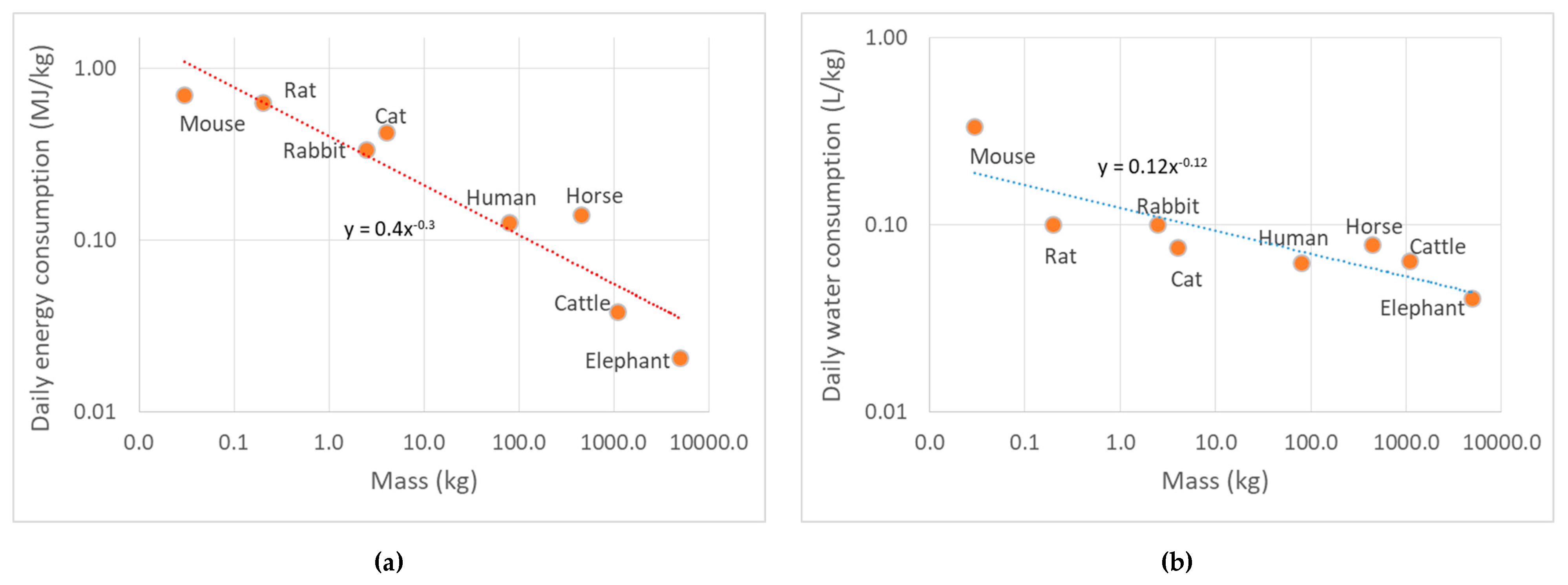
The first question has a seemingly straightforward answer. The plots in Figure 1 give a first positive reply to it. The average elephant, the biggest currently living animal on land, requires remarkably less energy per mass than a mouse in order to survive (Figure 1a) as the bigger the animal, the more efficiently it uses energy [6,7]. Larger scales also seem to increase efficiency for mammals in terms of water consumption for survival (Figure 1b). Clustering is also useful in human societies, as clustering of humans created what we now know as civilization. The clustering of human social processes along with their increase in spatial scale, is a primary principle for the societal world. This is because human clustering and interdependence structures enhance communication, promote science and exchange of ideas, boost trade and reduce the cost of basic social goods (such as access to water and energy), thereby improving the overall quality of human life [8,9,10]. In financial terms, the advantageous features of increased clustering are expressed through the classic concept of “economies of scale” [11].

A more holistic inspection of natural evolution however reveals hidden elements of clustering, which suggest that the second question also has a positive answer. Dinosaurs were the biggest living creatures on earth but about 66 million years ago they disappeared. Smaller animals such as mammals survived because of “Being small. If you’re small you probably have a large population and thus a wider genetic diversity.” [15]. Similar considerations might be drawn for human societies regarding the rise and fall of civilizations, the population and depopulation of large cities, followed by analogous trends in economic and agricultural activities over various spatial scales. The reasons behind the reverse trend in the clustering tendency might be less discernible for the anthropogenic world, however it becomes clear in this case as well that there is no single direction in terms of clustering but rather there is a certain stochastic element dominating its evolution.

With the stochastic tool 2D-Climacogram (2D-C), clustering is quantified from each image through cumulative variability over various scales, and a methodology is developed to allow the characterization of its temporal evolution. In the literature, there are many approaches to quantify clustering, calibrated for application in different fields as biology and ecosystems [16,17], life sciences [18,19,20,21], neural networks [22], physics and physical phenomena [23,24], maps [25,26] and more [27], yet there is no approach proposing a unifying stochastic view of 2D clustering in terms of variability vs. scale. Moreover, while the presence of 2D clustering is studied as a behavior, its temporal evolution is less explored as until recently, there was a scarcity of spatial information in time. Using various sources of spatial information, such as animated maps [28,29] and satellite images, an effort is made to characterize and interpret certain spatial aspects of the evolution of the natural and human world that provide quantitative insights for understanding the past. This understanding might serve as a basis for large-scale decision making for the future. This paper presents a stochastic methodology that quantifies clustering in 2D space and its temporal evolution by analyzing image sequences of the spatial structures over time.

We show the applicability of our tool in different fields by providing case studies from the analysis of clustering in ecosystems i.e., the evolution of forests and water bodies, of human structures, i.e., in terms of urbanization and urban expansion as well as in terms of cosmological simulations. The latter provide a very relevant quantification of clustering as the evolution of clustering in universe is widely studied [30,31,32,33,34] and it can be viewed as a macroscopic picture of clustering in nature.

We conclude our work with a theoretical discussion on the role of clustering in the human social structure. In view of the COVID-19 pandemic, we discuss the risk dynamics stemming from large-scale human clustering. Furthermore, by considering the way the latter was mitigated, i.e., through the destruction of large-scale social clustering structures, we draw wider considerations on the existence of an “optimal” scale and spatial distribution for human organization and society development.

2. Methodology

2.1. Stochastic Analysis of Clustering in 2D Space: The 2D-C Tool

The mathematical field of Stochastics has been introduced on the opposite side of deterministic approaches, as a way to model the so-called random, i.e., complex, unexplained or unpredictable, fluctuations observed in non-linear geophysical processes [35,36]. Stochastics helps to develop a unified perception of natural phenomena and expel dichotomies like random vs. deterministic. From the viewpoint of stochastics, there is no such thing as a “virus of randomness” that infects some phenomena to make them random, leaving other phenomena uninfected. Instead, both randomness and predictability coexist and are intrinsic to natural systems which can be deterministic and random at the same time, depending on the prediction horizon and the time scale [37]. This research aims to develop a stochastic analysis method to quantify both the spatial structures in terms of clustering and the temporal evolution thereof.

A stochastic computational tool called 2D-Climacogram, abbreviated as 2D-C [38,39], is used to study the clustering in 2D space, using images from various sources. 2D-C measures the degree of variability (change in variability vs. scale) in images using stochastic analysis. Here, we refer to spatial scale, defined as the ratio of the area of k × k adjacent cells (i.e., scale k) that are averaged to form the (scaled) spatial field, over the spatial resolution of the original field (i.e., at scale 1).

Image processing typically begins with filtering or enhancing an image using techniques to extract more information from the images [40] and image segmentation is one of the basic problems in image analysis. The importance and utility of image segmentation has resulted in extensive research and numerous proposed approaches based on intensity, color, texture etc. that are both automatic and interactive [41].

This analysis for image processing is based on a stochastic tool called climacogram. The term climacogram [42,43] comes from the Greek word climax (meaning scale). It is defined as the (plot of) variance of the averaged process (assuming stationary) versus the averaging scale k and is denoted as γ(k). The climacogram is useful for detecting both the short- and the long-term change (or else dependence, persistence and clustering) of a process, with the latter emerging particularly in complex systems as opposed to white-noise (absence of dependence) or Markov (i.e., short-range dependence) behavior [44].

In order to quantify the image variability, each image was first digitized in two dimensions (2D) based on the grayscale color intensity (thus, studying the brightness of an image), and the climacogram was calculated based on the geometric scales of adjacent pixels. Assuming that our sample is an area nΔ × nΔ, where n is the number of intervals (e.g., pixels) along each spatial direction and Δ is the discretization unit (determined by the image resolution, e.g., pixel length), the empirical classical estimator of the climacogram for a 2D process can be expressed in equation 1 as:

$$\underset{\_}{\widehat{\gamma }}\left(\kappa \right)=\frac{1}{n^2/{\kappa }^2-1}{\displaystyle \sum }_{i=1}^{n/\kappa }{\displaystyle \sum }_{j=1}^{n/\kappa }{\left({\underset{\_}{x}}_{i,j}^{\left(\kappa \right)}-\overline{\underset{\_}{x}}\right)}^2$$

(1)

where the ‘^’ over γ denotes an estimate, $\kappa$ is the dimensionless spatial scale, ${\underset{\_}{x}}_{i,j}^{\left(\kappa \right)}=\frac{1}{{\kappa }^2}{\displaystyle \sum }_{\psi =\kappa \left(j-1\right)+1}^{\kappa j}{\displaystyle \sum }_{\xi =\kappa \left(i-1\right)+1}^{\kappa i}{\underset{\_}{x}}_{\xi ,\psi }$ represents a local average of the space-averaged process at scale κ, and at grid cell (i,j), $\overline{\underset{\_}{x}}\equiv x_{1,1}^{\left(n\right)}$ is the global average and the underlined variables represent random variables as opposed to regular ones. Note that the maximum available scale for this estimator is n/2. The difference between the value in each element and the field mean is raised to the power of 2, since we are mostly interested in the magnitude of the difference rather than its sign, and in particular, in the variance estimation. Therefore, the 2D-C expressed the diversity in the color intensity among the different elements at each scale by quantifying the variability of their brightness intensities.

An important property of stochastic processes which characterizes the variability over scales is the Hurst–Kolmogorov (HK) behavior (persistence), which can be represented by the Hurst parameter [45]. This parameter can be estimated by minimizing the fitting error between the empirical (observed) and the modeled (Equation (2)) climacogram, both of which are derived from the large-scale values, i.e., the last 50 scales are used in the presented applications. The isotropic HK process with an arbitrary marginal distribution, i.e., the power-law decay of variance as a function of scale, can be defined for a 1D or 2D process as:

$$\gamma \left(k\right)=\frac{\lambda }{{(k/\Delta )}^{2d\left(1-H\right)}}$$

(2)

where $\lambda$ is the variance at scale k = Δ, Δ is the time or space unit, d is the dimensionality of the process/field (i.e., for a 1D process d = 1, for a 2D field d = 2, etc.) and H is the Hurst parameter (0 < H < 1). For 0 < H < 0.5 the HK process exhibits an anti-persistent behavior, H = 0.5 corresponds to the white noise process and for 0.5 < H < 1 the process exhibits persistence (i.e., clustering). In the case of clustering behavior due to heterogeneity of the brightness of the image, the high variability in brightness persists even in large scales. This clustering effect may substantially increase the diversity between the brightness in each pixel of the image, a phenomenon also observed in hydrometeorological processes (such as temperature, precipitation, wind etc. [36]), natural landscapes and music [46].

The algorithm that generates the climacogram in 2D was developed in MATLAB for rectangular images [47]. In particular, for the current analysis, the images are cropped to 400 × 400 pixels, 14.11 cm × 14.11 cm, in 72 dpi (dots per inch).

2.2. Temporal Evolution of 2D Clustering

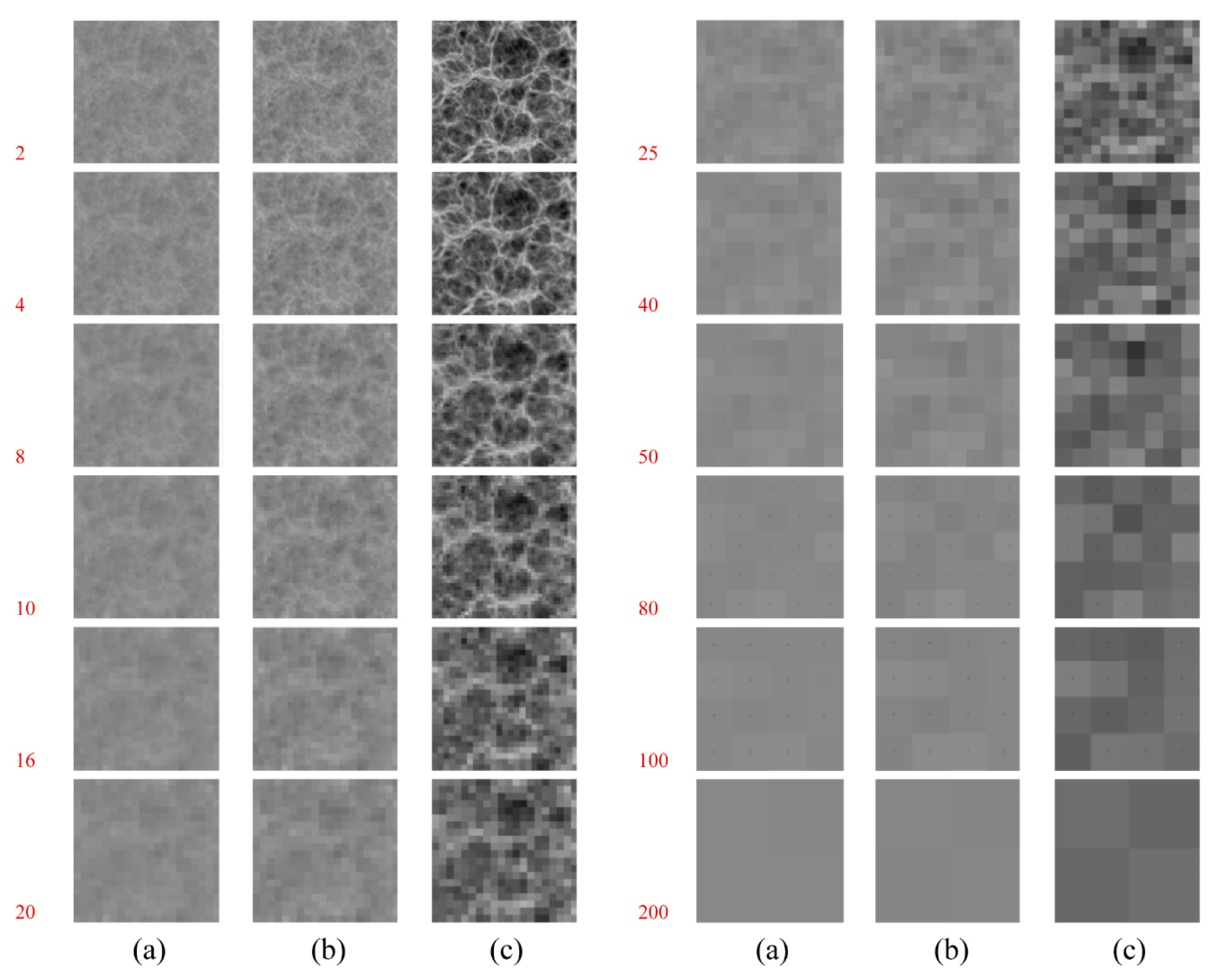
The pixels analyzed are represented by numbers denoting their color intensity in grayscale (white = 1, black = 0). Figure 2 presents images from three timeframes of the evolution of the universe as generated by a cosmological model of evolution [48]: (a) 500 million years after Big Bang, an image with faint clustering; (b) 1000 million years after the Big Bang, an image with clustering and (c) 10,000 million years after the Big Bang, an image with intense clustering. Figure 3 presents the steps of analysis and shows grouped pixels at scales k = 2, 4, 8, 16, 20, 25, 40, 50, 80, 100 and 200 that were used to calculate the climacogram.

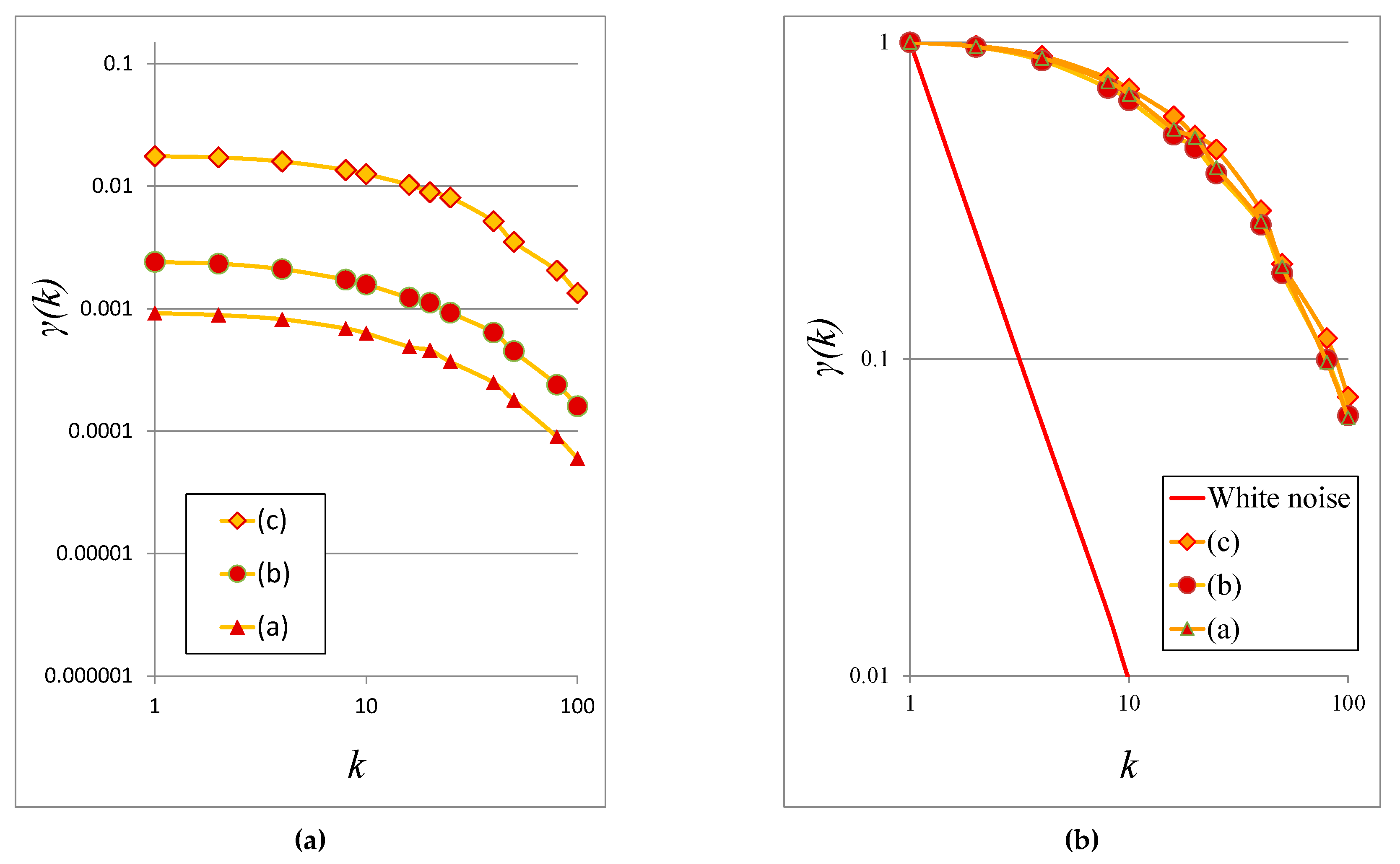
The presence of clustering is reflected in the climacogram, which shows a marked difference as clustering increases (Figure 4a,b). Specifically, the variance of the images is notably higher at all scales when clustering increases, indicating a greater degree of variability of the process.

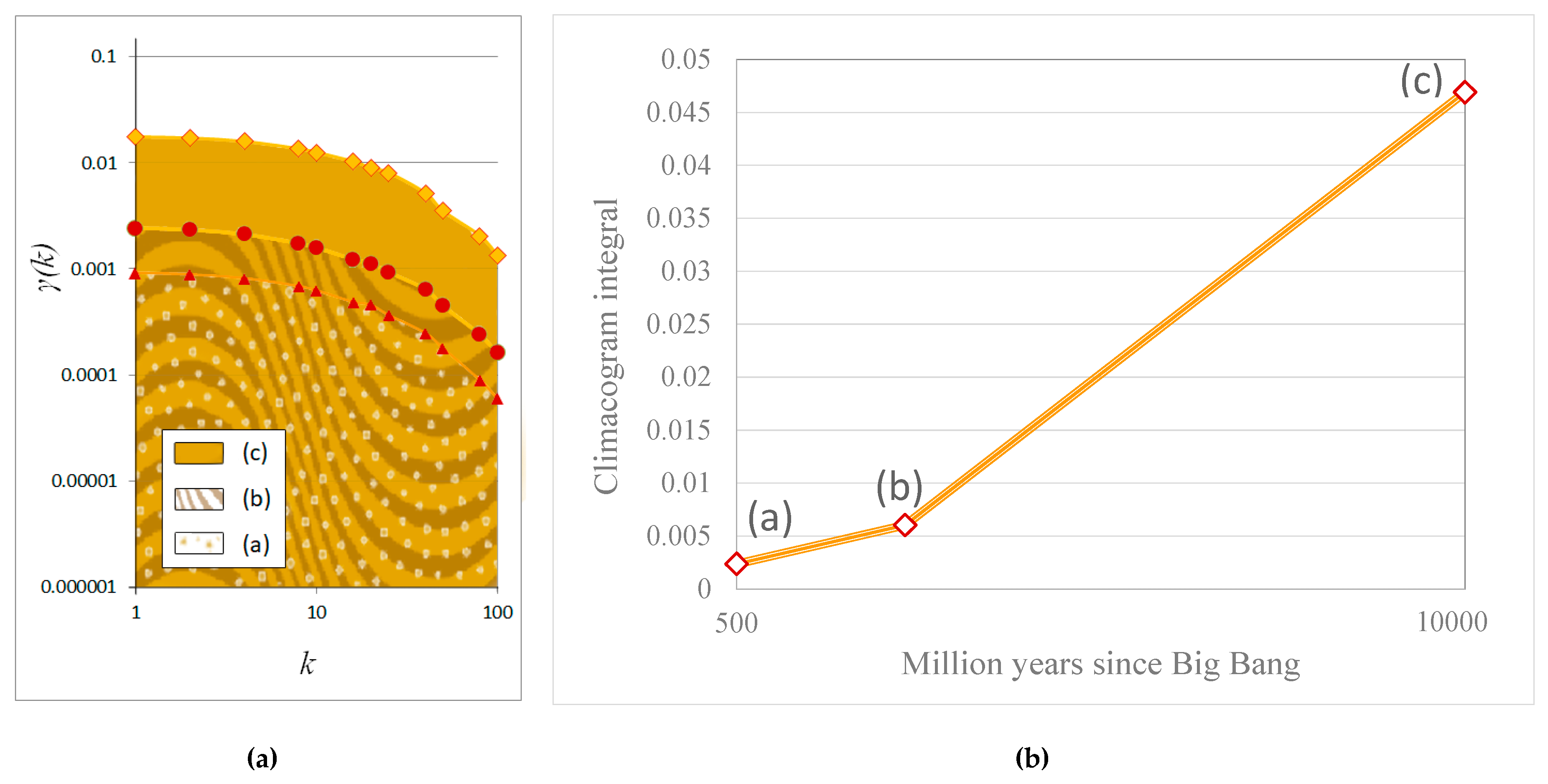
For the integration of all information contained in the 2D climacogram of each timeframe, we evaluated the cumulative areas underneath each one for all scales (Figure 5a), i.e., the climacogram integral ${{\displaystyle \int }}_{\Delta }^k\gamma \left(x\right)/x \mathrm{d}x$, where Δ and k are the minimum and maximum scale and we have divided by x in order for the integral to converge for an arbitrarily high k ($k\to \infty$). In the discrete case, this can be approximated as in Equation (3):

$$\mathrm{CI}\left(k\right)={\displaystyle \sum }_{i=1}^{n\left(k\right)-1}2\gamma \left(x_i\right)\frac{x_{i+1}-x_i}{x_{i+1}+x_i}$$

(3)

where $n\left(k\right)$ is the number of integration intervals up to scale k. We evaluated $\mathrm{CI}\left(k\right)$ at the maximum available spatial scale, in order for it to be the best approximation of the limit $\mathrm{CI}(\infty )$.

In Figure 5b, each climacogram is represented by the respective integral, thus we can evaluate the rate of alteration of clustering through time.

3. Case Studies

In order to present the applicability of our tool in different fields, we studied several examples as case studies illustrating clustering in nature from cosmological simulations as well as in ecosystems and human social structures such as the evolution of urbanization and urban expansion.

3.1. Evolution of Clustering in Nature

3.1.1. Cosmological Simulations

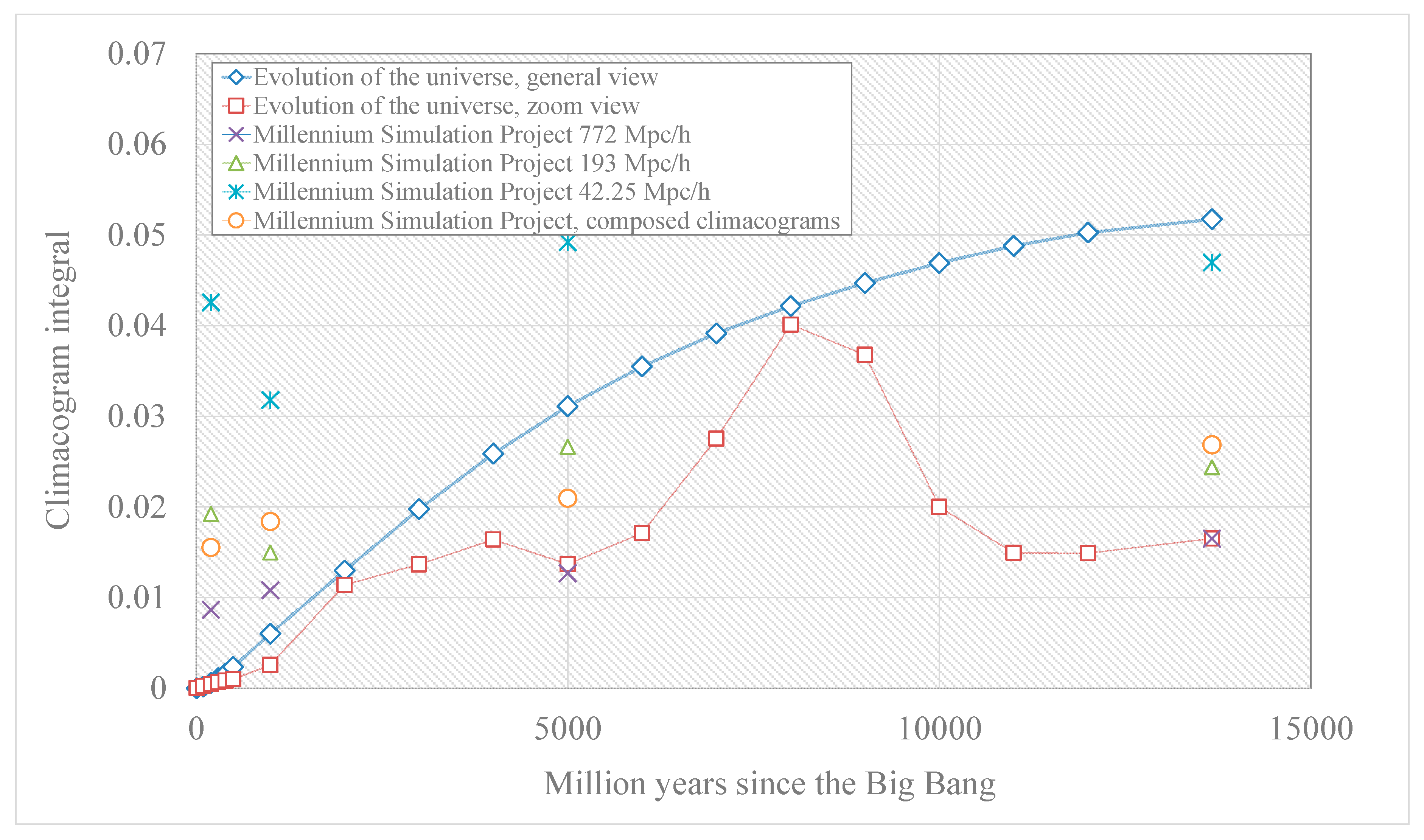
Some cosmological simulations of the growth of Black Holes and Galaxies [48] show that the evolution of the universe is characterized by a tendency for clustering through time [34]. We analyzed timeframes of a general view of one cosmological simulation model (Figure S1: General view of the direct Cosmological Simulations of the Growth of Black Holes and Galaxies [48,49]) and a closer zoom (Figure S3: Closer zoom in an area of the direct Cosmological Simulations of the Growth of Black Holes and Galaxies) using 2D-C plots (Figure S2: Climacograms of the Direct Cosmological Simulations of the Growth of Black Holes and Galaxies (Figure S1) and Figure S4: Climacograms of the closer zoom of Direct Cosmological Simulations of the Growth of Black Holes and Galaxies (Figure S2)). We evaluated the temporal evolution of clustering by following the methodology of Section 2, i.e., we found the cumulative areas underneath each time-referenced climacogram and plotted the temporal evolution of the integrals (Figure 6).

In addition, we evaluated the clustering behavior shown in the Millennium Simulation Project [50] (Figure S5: Evolution of the universe. Millennium Simulation Project [50]). Specifically, the Millennium simulation Project shows four timeframes of the evolution of a projected density field, with three different views. To unify the study of the stochastic behavior from the three distinct cosmological views of Millennium Simulation Project (772 Mpc/h, 193 Mpc/h, 48.25 Mpc/h) we employed the following procedure. For each scale, we formed the sample of empirical climacogram values estimated from each of the three series. For the range of scales at which the series overlap we matched the respective climacogram values with one another by minimizing the sum of their sample standard deviations for the given scales. For the (unconstrained) minimization we used the Generalized Reduced Gradient method [51,52] which is one of the most robust and reliable approaches to nonlinear optimization [53] (Figure S6: Fitting curves of composed climacograms of Millennium Simulation Project [50] (a) image series of 210 mil years after B.B.; (b) image series of 1000 mil years after B.B.; (c) image series of 4700 mil years after B.B.; (d) image series of 13,600 mil years after B.B.).

3.1.2. Ecosystems

Ecosystems are characterized by dynamic transformations involving spatial clustering. In order to show how the proposed stochastic tool could be applied in the study of ecosystems, we present the quantification of the evolution of clustering for three case studies:

• the deforestation of Borneo, Figure 7, Figure 9a, Figure S8: Deforestation in Borneo 1950–2005 (a) 1950; (b) 1985; (c) 2000 (d) 2005 [54], Figure S9: Climacograms of the deforestation in Borneo, Figure S10: Evaluation of climacograms and rhythm of clustering in demolition of fosters’ clustering in Borneo,
• the deforestation of the Amazon, Figure 8, Figure 9b, Figure S11: Deforestation of Amazon, creation of clustering of dry land and urban areas inside forest [55], Figure S12: Climacograms of the deforestation in Amazon, Figure S13: Evaluation of climacograms and rhythm of clustering evolution of dry-lands’ clustering in Amazon
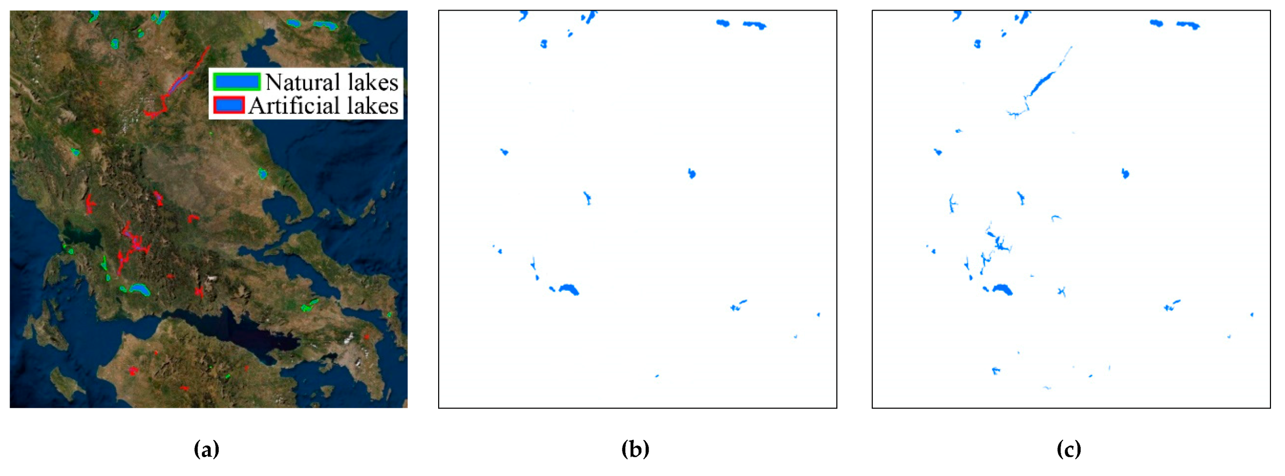
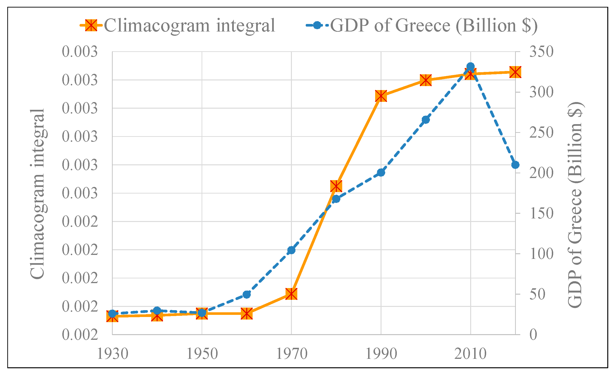
• the evolution of water bodies in Greece, Figure 10, Figure 11, Figure S14: Greece, natural and artificial lakes (a) overview map of the area with natural and artificial lakes in 2020; (b) layer of the map; natural and artificial lakes 2020; (c) layer of the map; lakes 2020, Figure S15: Evolution of water bodies in Greece as new big dams are constructed and new artificial lakes are created, Figure S16: Climacograms of the evolution of water bodies in Greece.

In these examples, we can see the demolition of the forests’ clustering in Borneo, and the evolution of clustering of dry lands and urban areas in the Amazon forest. An interesting insight is provided, showing the evolution of water bodies in Greece, as new artificial lakes are created, resulting in amplification of natural variability. Such an argument in favor of the integration of dams in the landscape was recently proposed [56]. Note that increasing clustering of water bodies is associated with the construction of large-scale dams and it is related to the economic growth; increasing clustering appears in periods of increasing Gross Domestic Product (GDP) (Figure 11).

3.2. Evolution of Human Social Clustering

Large-scale infrastructure projects are necessary when the human population is clustered and organized in large units. In order to understand and describe the changing scale of infrastructures, it is necessary to first assess the evolution of human social clustering. This is facilitated through the investigation of spatial databases. To this aim, we employed our stochastic methodology to characterize the temporal evolution of spatial information regarding human social clustering.

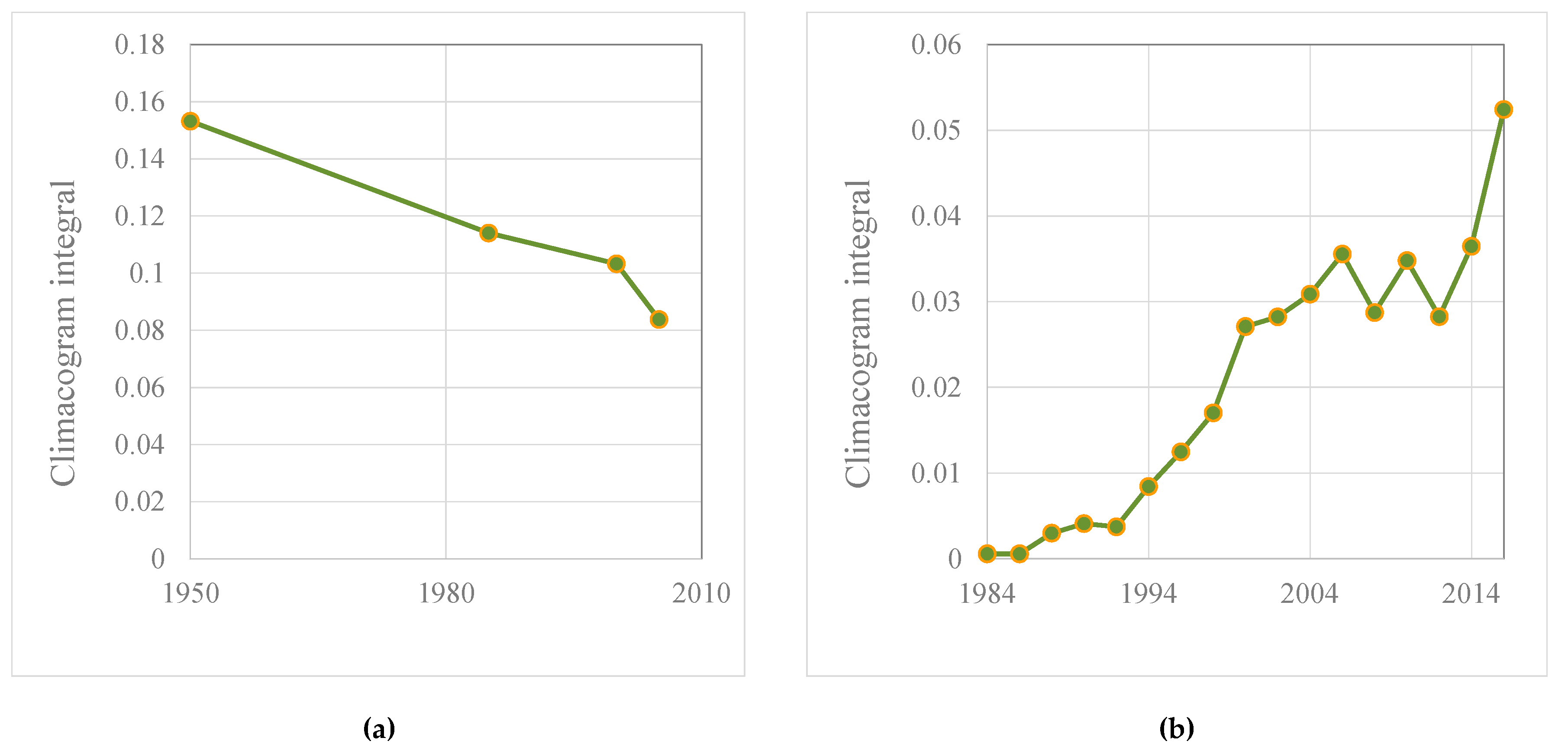
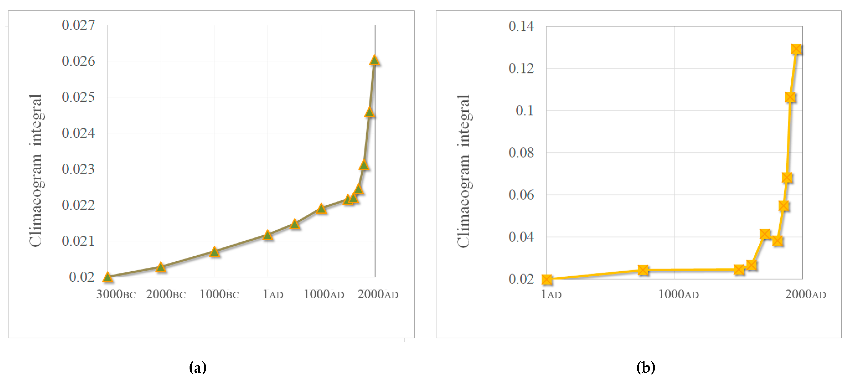
The beginning of human civilization is signaled by the organization of systematic agriculture through the clustering of cropland areas (Figure 12, Figure S18: Evolution of cropland area; historical data from 3000 BC to AD 2000. [57]) and the formation of human clustering structures, i.e., societies that stabilized in space forming cities and transforming their environment (Figure 13, Figure S20: Evolution of London; historical data from 1 AD to 1950 AD. [58]). We evaluated related historical data to quantify the evolution of clustering at the global (Figure 14a, Figure S19: Climacograms of cropland areas, Figure S22a: Evaluation of climacograms and rhythm of clustering of cropland land historical data) and local scale (Figure 14b, Figure S21: Climacograms. Clustering of urbanization of London, Figure S22b: Evaluation of climacograms and rhythm of clustering and evolution of urbanization in London area).

Figure 14a shows the evolution of cropland areas from 1000 BC to 2000 AD worldwide, derived from [57], whereas Figure 14b shows the evolution of settlements in London from 1 AD to 1900 AD, derived from [58]. It is interesting to note the radical increase in the rate of clustering occurring in both cases after 1700 AD (Figure 14), i.e., in the period after the industrial revolution.

It should be noted however that threats such as natural disasters and war demolish clustering of human social structures, as revealed by the inspection of satellite lights in Syria after the onset of the civil war (Figure 15, Figure S40: Satellite night lights of Syria taken from Reference [59]; (a) 2012; (b) 2014; (c) Rate of alteration of clustering after the onset of the civil war).

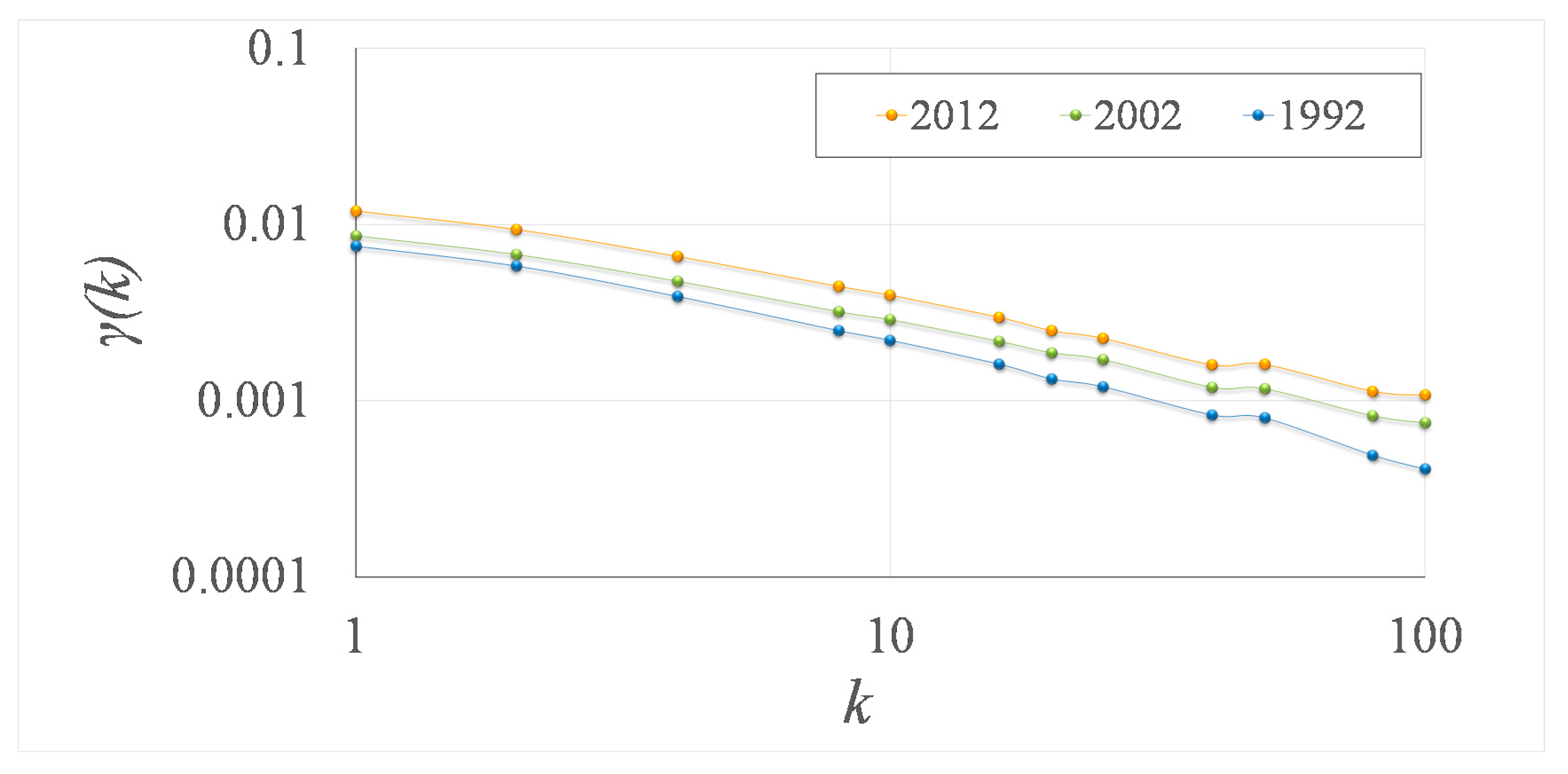
Next, we explored spatial data pertaining to urbanization taking place in the past century. The first information source examined was the spatial distribution of satellite night lights. The night lights have been widely used as an index of the population and density of settlements [60], economic activity [61], consumption and distribution of electricity [62], poverty and development status [63] and human exposure to natural disasters such as floods [64]. An example showing satellite images from city lights in Europe is shown in Figure 16, while their respective climacograms are shown in Figure 17.

The second information source examined was the spatial dataset on land uses. Large-scale geospatial data, including land-cover types, were obtained from the Historical Database of the Global Environment, HYDE 3.1 [57], of the National Centers For Environmental Information at the National Oceanic And Atmospheric Administration (NOAA). HYDE datasets are based on Food and Agriculture Organization of the United Nations agricultural statistics and land use (FAOSTAT) over the period 1960–2010 [65], a variety of other historical information prior to 1960, datasets for wood harvest by FAO and urban land extent [57] in combination with assumptions of other land cover change (e.g., forest areas, which are estimated by MODIS equipped satellites). This dataset was chosen because it contains valuable temporal information on urbanization.

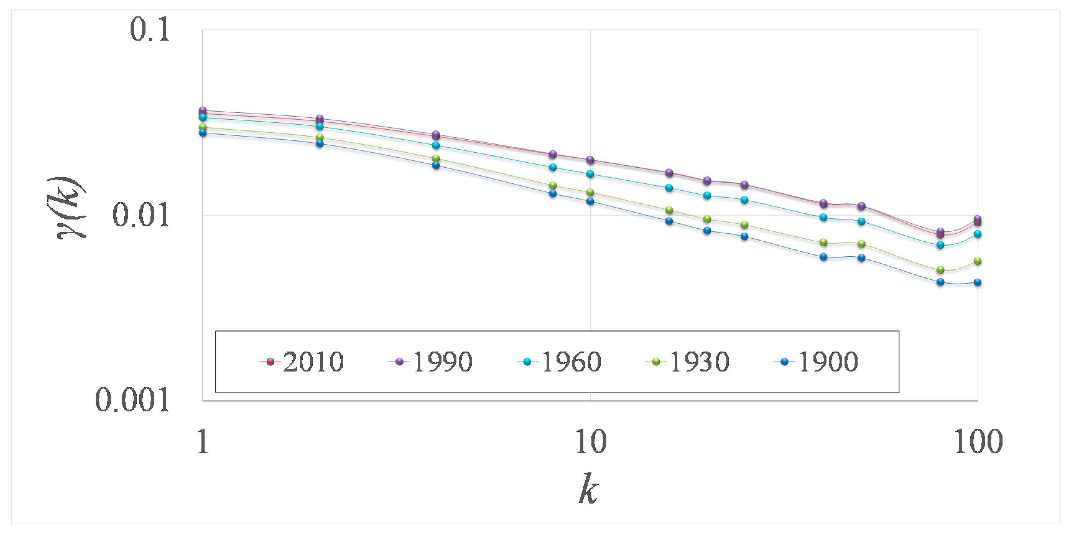
The land cover dataset was provided in form of NetCDF files at a spatial resolution of 0.5 × 0.5 degrees of latitude and longitude. Therefore, the size of each grid cell expands from 1.3475 × 10⁷ m² to 3.088224 × 10⁹ m². In addition, land cover geospatial data were provided at an annual time resolution using the WGS84 reference coordinate system. The longest record spans the years 1770–2010, but our studied period spans from 1900 to 2010. Land cover annual maps report the percentage of grid cell areas belonging to each of 28 land cover types, from which we focus on the urban land cover type. An example showing the extension of urban land cover in Europe is shown in Figure 18, while their respective climacograms are shown in Figure 19.

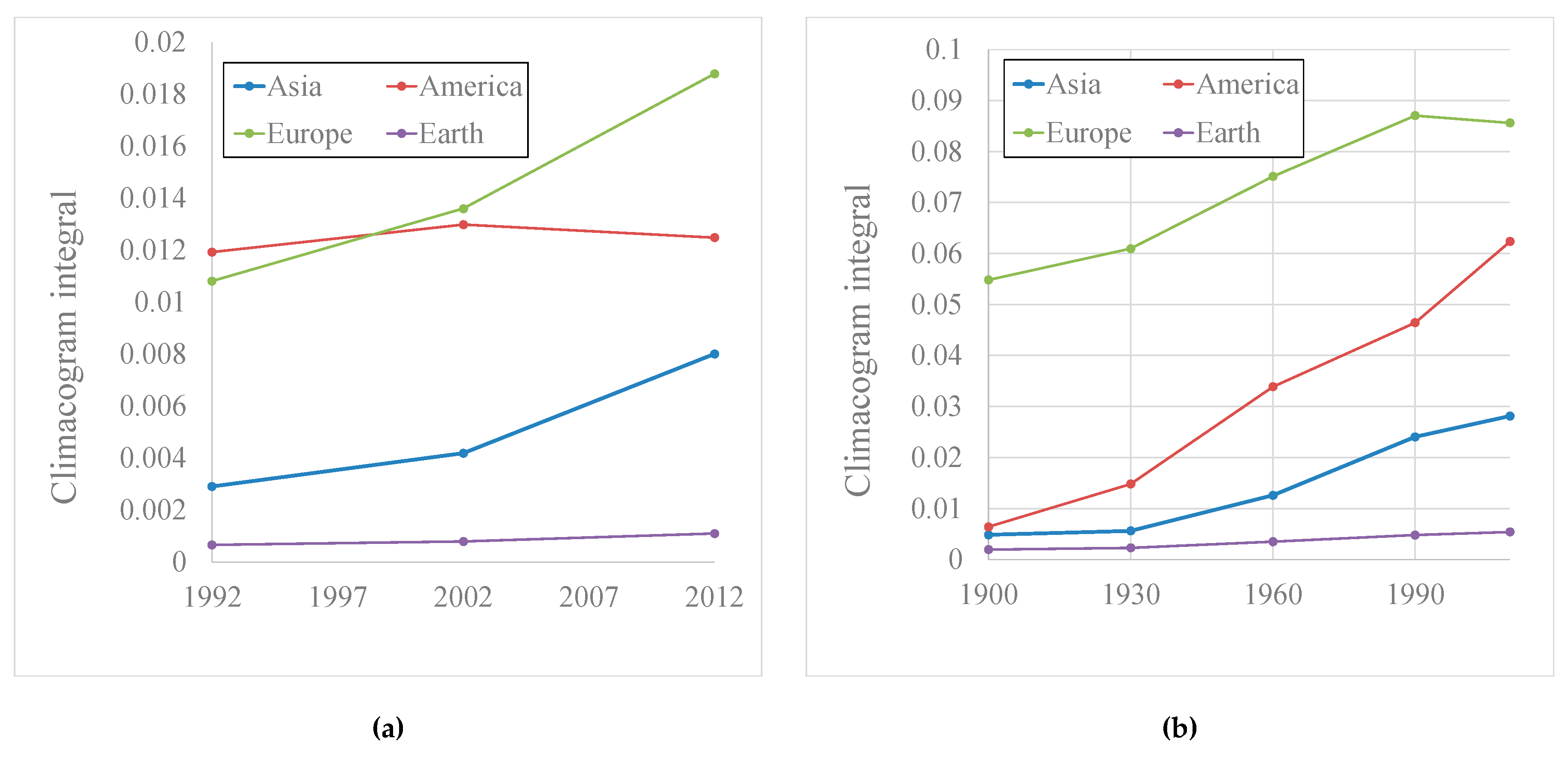
All studied images along with the complete climacogram analysis for Europe, Asia, America and the globe is presented in the Supplementary Material (Figures S23–S39) and summarized in Figure 20.

The temporal evolution of human social clustering from both information sources is presented in Figure 20. Overall, the analyses support the case for increased human social clustering during the 20th century in all three continents, i.e., Asia, Europe and America. A few differences arise from the comparison of the period that the information sources overlap, i.e., from the 1992 to 2010. Namely, although urbanization appears increasing in terms of land use in America, this trend is not confirmed by the evaluation of night lights for the same period, which appear to have slightly decreased. In contrast, the night lights in Europe have majorly increased during this period, despite the relative stability in the urban land use cover. These differences indicate the virtue of considering both information sources, as night lights appear to be a better index of population density, whereas the land use cover is more reflective of the spatial expansion of urban land uses. From this point of view, it appears that urban expansion has been more prominent in America, whereas Europe has experienced increased population density. Last, Asia shows consistent increases in both information sources over the last few decades.

4. Discussion

4.1. Human Social Clustering as a Means for Development and Progress

The idea of economies of scale as developed by Adam Smith [66] is that with the increase of growth comes a decrease of the cost per unit [10]. The advantages of economies of scale have theoretical limits, i.e., when reaching the optimal design point where the cost per additional unit begins to increase. Economies of scale are related to scale development of infrastructures where there are also additional limits induced due to lack of funds, technical difficulties as well as public opposition [67] and resources accessibility. Large scales of infrastructure have risks [68] but are also advantageous for local economies [69]. Previous work [8] has shown that changing the scale of water infrastructures results to changes in the cost of water in agreement with the so-called “0.6 rule” in macroeconomics [8,70,71].

This relationship is also addressed by Wenban–Smith [72], who uses the term “density effects” to describe the clustering trend towards concentration of population and large scales infrastructures. For instance, in Greece we can see this clustering trend in terms of infrastructure in the construction of large-scale dams. Other emblematic examples of large-scale projects include the controversial “North American Water and Power Alliance” [73,74] (not constructed yet), Tehri Dam [75] (constructed in India) and the Three Gorges Dam [76] (constructed in China).

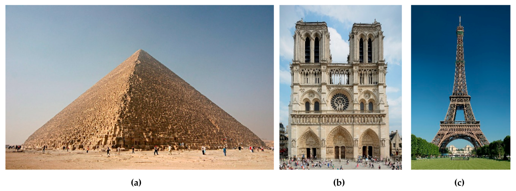
In order to solve the problem of the optimal scale of infrastructure, multi-criteria optimization is required. Despite the contributions of mathematicians, little progress has been made in this engineering problem until the last half of the 20th century, when high-speed digital computers made it possible to apply optimization techniques to large-scale structures with powerful and popular complex optimization methods [77]. Still, it is often the case that rather than cost-benefit optimization, political and aesthetical reasons (as the desire for creation of civilization signals), are the driving forces behind the choice of the scale of historical infrastructures; notable examples are shown in Figure 21.

What is common though in these large-scale projects, is the existence of an efficient state structure able to take the relevant decisions about political and administrative mechanisms for decisions clustering, as well as to impose and finance them. Thus, they reflect the presence of a stable social mechanism which, according to the theory of Tomas Hobbes [81], is represented by Leviathan. The latter metaphorically represents a central political entity that seeks to preserve law and peace by imposing a utilitarian egoism driven by the instinct of self-preservation (conatus) and the will to dominate, exercising absolute power only in favor of preserving social peace, i.e., the well-known social contract. Leviathian also undertakes the protection of citizens from external and internal factors, while also protecting citizens from the central entity itself. From this idea the Constitution originated as a self-limitation of power. As engineering development is intertwined with social peace and prosperity, we can assume that a form of centralized socio-political structure the likes of Leviathan is required in order to undertake decisions about large-scale development and infrastructure projects.

Another view on the creation of large infrastructure projects through centralized social structures is given by Aristotle [82]: “...καὶ τὸ πένητας ποιεῖν τοὺς ἀρχομένους τυραννικόν, ὅπως μήτε φυλακὴ τρέφηται καὶ πρὸς τῷ καθ᾽ ἡμέραν ὄντες ἄσχολοι ὦσιν ἐπιβουλεύειν. παράδειγμα δὲ τούτου αἵ τε πυραμίδες αἱ περὶ Aἴγυπτον καὶ τὰ ἀναθήματα τῶν Κυψελιδῶν καὶ τοῦ Ὀλυμπίου ἡ οἰκοδόμησις ὑπὸ τῶν Πεισιστρατιδῶν, καὶ τῶν περὶ Σάμον ἔργα Πολυκράτεια (πάντα γὰρ ταῦτα δύναται ταὐτόν, ἀσχολίαν καὶ πενίαν τῶν ἀρχομένων)”. English translation [83]: “And it is a device of tyranny to make the subjects poor, so that a guard may not be kept, and also that the people being busy with their daily affairs may not have leisure to plot against their ruler. Instances of this are the pyramids in Egypt and the votive offerings of the Cypselids, and the building of the temple of Olympian Zeus by the Pisistratidae and of the temples at Samos, works of Polycrates (for all these undertakings produce the same effect, constant occupation and poverty among the subject people)”. This example highlights the mutually dependent relation between central entities and large-scale development: the existence of the one often relies on the other.

4.2. Risks From Large-Scale Clustering

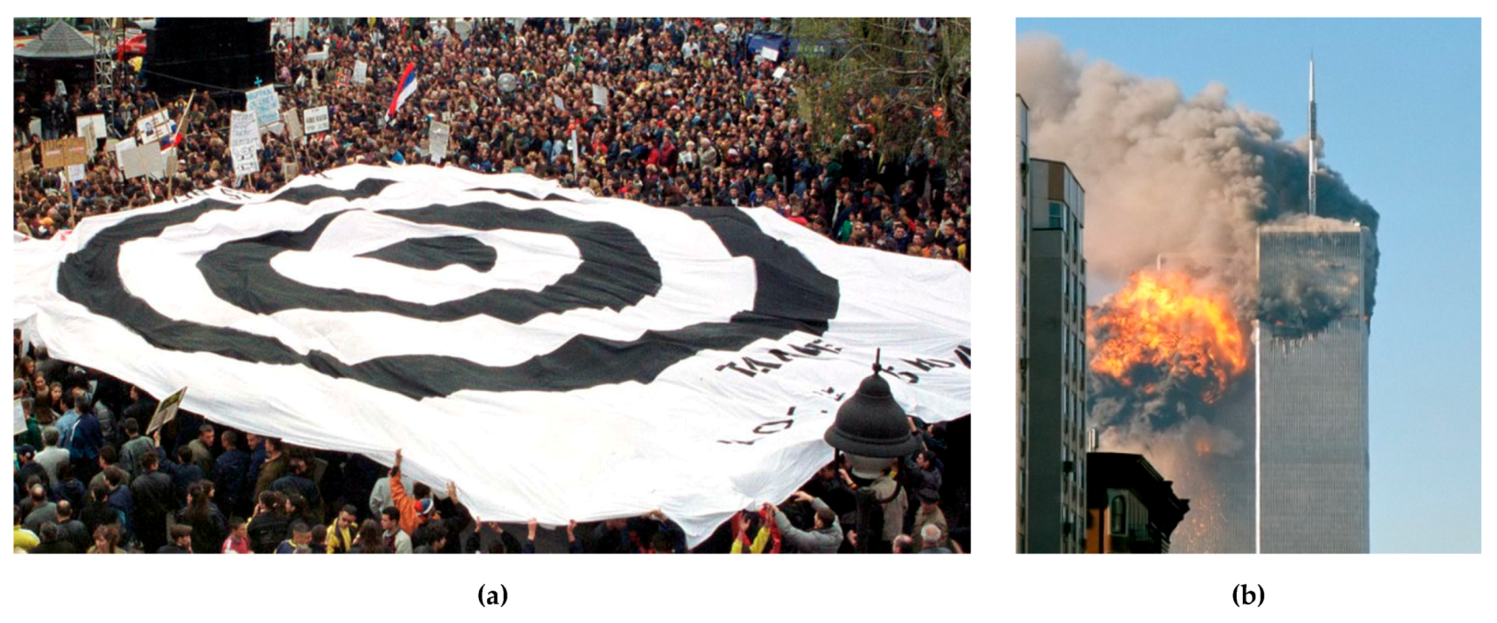
While human social clustering increases the chances for social progress and prosperity, it also increases exposure and vulnerability to different kinds of risk. For the first time in human history, more people live in cities than in rural areas. This rapid growth in the number of people living in cities and urban landscapes is increasing the world’s susceptibility to natural disasters [84,85] and other threats [86]. For instance, in the case of war, large-scale infrastructure projects are important and common targets. Figure 22a depicts Serbian civilians, forming human shields to protect their country’s infrastructure during the NATO bombing of Yugoslavia during the Kosovo War (1999). Large-scale infrastructures are also symbols of civilizations and this is why the World Trade Center was a target during the 9/11/2001 attack (Figure 22b).

On the other hand, modern large-scale infrastructure projects have a life of no more than 120 years due to aging of their materials and the difficulties in maintaining them [87]. As a simple example, consider the two collapses of large-scale bridges that have occurred in Italy in the past few years, causing fatalities and massive disruption of transportation [88,89]. Moreover, it is straightforward to see how a possible failure in large-scale water-supply infrastructures upon which societies are heavily reliant would create a vague gap in social functioning [88].

It is therefore evident that with the increase of the scale of the development along with the planned increase of benefits comes also an increase of risks, as the concentration of goods and services in one place makes the human communities more vulnerable to a destruction of this supply chain. Interestingly, metaphors on the existence of a limit in the scale of human works are present in various literature and theological works since antiquity, perhaps the most famous examples are found in the Holy Bible. In the latter the man is regarded as the crown of God’s Creation and by the fall of man in Original Sin, the whole Creation falls (Genesis 3.17 [90], St Paul, Epistle to the Romans; 8.20-22. [91]). After the fall of humans, the environment became hostile and man had to do work to survive. In the famous myth of the Babel tower, the Holy Bible explicitly communicates the notion of an upper limit in the scale of human works (Genesis 11, Job 38:1-41 [90]).

Recently, due to the ongoing COVID-19 pandemic, we have been collectively reminded of how large-scale human social clustering increases the risk of pandemics. In the developed world, the majority of measures to mitigate the spread of the pandemic have been based on forms of social distancing, with lock-downs being the ultimate measure. Nearly three billion people were in quarantine in April 2020 [94]. In this respect, the Epicurean philosopher Lucretius says that if there is no immediate risk of death, people are not afraid of death [95], but the fear of death can lead people to make social divisions and suspend their personal growth [96]. Indeed, when people are afraid of dying, it is common to believe that the avoidance of social contact will help them avoid danger, illness and death altogether. This phenomenon is well documented in social fear management studies [97] and in this context, it can also be viewed as another implicit communication of the risks of social clustering.

5. Conclusions

It is argued herein that clustering is both a natural and a human social tendency that comes with different qualitative consequences with scaling, i.e., the properties of large scales cannot be derived from the ones of small scales. In these terms, as both the scales of current societies and that of engineering projects increase, it is of paramount importance to understand both the structure of spatial clustering and its temporal evolution. To this aim, this research develops a stochastic method of general applicability for the quantification of the temporal evolution of spatial clustering as a tool to assess, monitor and potentially predict elements of global changes.

The tool called 2D-C (2D-Climacogram) quantifies the variability of images through the variance of the brightness intensity in grayscale. Upon a careful selection of images representing spatial information, we can derive a quantification of clustering over time that is useful for either quantitatively characterizing known spatial changes, as urbanization, and tracking their temporal evolution, or even revealing spatial patterns that are less expected, i.e., pertaining to feedback loops between anthropogenic interventions and natural variability. We present a range of applications for (a) the natural sciences, in terms of the evolution of the universe as suggested by cosmological simulations and of ecosystems, such as forests and lakes, and (b) for human sciences dealing with social structures, as revealed by the evolution of worldwide cropland data, satellite images of night lights and spatial data on urban land cover.

Our results support the concept that there is a tendency for clustering both in the natural and anthropic world, yet this tendency is scale-dependent as beyond a certain scale it may as well be dissolved or replaced by a structure of another quality. We have seen that in the evolution of the universe clustering increases and decreases depending on the scale of view, and structures that have grown and seem at a certain scale to be merging (galaxies, clusters, super clusters, etc.), in other scales are moving apart. In biological life clustering is related to saving of energy resources, as in in mammals, but it is not always stable; for instance, dinosaurs disappeared. The case studies on ecosystems, namely the Borneo and Amazon forests and the lakes in Greece, show that the clustering method offers an effective characterization of the evolution of ecosystems revealing clustering and declustering patterns. In many cases, the interplay of natural and human-driven variability is difficult to discern and proves unpredictable in terms of evolution. Such a counterintuitive case is the found increase in ecosystem variability stemming from anthropogenic interventions such as dams.

Clustering and declustering periods are apparent in nature as also revealed by our case studies, as well as in human social structures. There are local examples of declustering, i.e., related to wars, famines or nuclear and natural disasters, but our case studies show an overall positive clustering trend. Specifically, in our study of long-term worldwide cropland data and London’s evolution, we have found that the rhythm of clustering dramatically increased since the industrial revolution, whereas urbanization followed this overall positive trend till the present time. This is in accordance with the widespread belief that larger human clustering structures enhance efficiency (e.g., through economies of scale). Yet it is becoming increasingly evident that clustered human structures come with increased risks as well. For instance, in the economy increasing clustering comes with increase in systemic risks, while centralization of infrastructure and resources increases vulnerability of the population during failure or war. In this period, the society is forced to radically reassess the clustering structures in different social scales in order to tackle the risk from the COVID-19 pandemic.

Despite the vast benefits resulting from centralized social structures during the last centuries as presented in Figure 14 and Figure 20, at this point in time, it is tempting to consider an alternative social distribution in space, perhaps a sparser and more decentralized one, taking example of the evolution of natural structures that are driven by uncertainty. The COVID-19 circumstance presents an opportunity to reconsider the trade-offs resulting from our natural tendency to cluster in space. In addition, it is an opportunity to revise the criteria for selecting the optimal scale for development, as well as the meaning that terms such as sustainability bear under unprecedented conditions.

In any case, the answer to the question of an optimal scale of social organization and development, is a fascinating problem that engineers among others, are urged to set and solve [98,99,100]. Homo Sapiens survived the natural selection being a (small-scale) mammal and not a (large-scale) dinosaur. Yet humans were ultimately able not only to adapt to new conditions but also to shape new conditions and modify their environments through science and technology.

References

1. Homer, Odyssey. Available online: http://users.uoa.gr/~nektar/arts/tributes/omhros/od17.htm (accessed on 15 September 2020).
2. A Brief History of Dinosaurs. Available online: https://www.livescience.com/3945-history-dinosaurs (accessed on 3 February 2020).
3. Mammal. Available online: https://en.wikipedia.org/wiki/Mammal (accessed on 3 February 2020).
4. Upham, N.S.; Esselstyn, J.A.; Jetz, W. Mammals Inferring the mammal tree: Species-level sets of phylogenies for questions in ecology, evolution and conservation. PLoS Biol. 2019, 17. [Google Scholar] [CrossRef] [PubMed]
5. Urushihara, H. Developmental biology of the social amoeba: History, current knowledge and prospects. Dev. Growth Differ. 2008, 50. [Google Scholar] [CrossRef] [PubMed]
6. Kleiber’s Law. Available online: https://en.wikipedia.org/wiki/Kleiber%27s_law (accessed on 17 January 2020).
7. Of Mice and Elephants: A Matter of Scale. Available online: http://courses.missouristate.edu/chrisbarnhart/bio121/lab/respiration/of_mice_and_elephants.htm (accessed on 12 January 2020).
8. Sargentis, G.-F.; Ioannidis, R.; Karakatsanis, G.; Sigourou, S.; Lagaros, N.D.; Koutsoyiannis, D. The Development of the Athens Water Supply System and Inferences for Optimizing the Scale of Water Infrastructures. Sustainability 2019, 11, 2657. [Google Scholar] [CrossRef] [Green Version]
9. Sargentis, G.-F.; Dimitriadis, P.; Ioannidis, R.; Iliopoulou, T.; Frangedaki, E.; Koutsoyiannis, D. Optimal utilization of water resources for local communities in mainland Greece (case study of Karyes, Peloponnese). Procedia Manuf. 2020, 44, 253–260. [Google Scholar] [CrossRef]
10. Koutsoyiannis, D. Scale of water resources development and sustainability: Small is beautiful, large is great. Hydrol. Sci. J. 2011, 56, 553–575. [Google Scholar] [CrossRef]
11. Koutsoyiannis, A. Modern Microeconomics, 2nd ed.; Springer: London, UK, 1979. [Google Scholar]
12. Asian Elephant Nutrition. Available online: https://asianelephantnutrition.wordpress.com/2015/02/25/big-body-lots-of-energy-maintenance/ (accessed on 18 January 2020).
13. Energy Requirements of Adult Cats. Available online: https://www.cambridge.org/core/journals/british-journal-of-nutrition/article/energy-requirements-of-adult-cats/225A91E97C8B94CAB4A5BF0646EFA2A2/core-reader (accessed on 18 January 2020).
14. Nutrient Requirements of Laboratory Animals. Available online: https://www.ncbi.nlm.nih.gov/books/NBK231925/ (accessed on 18 January 2020).
15. How to Survive Mass Extinction. Available online: https://www.theguardian.com/science/lost-worlds/2012/sep/20/dinosaurs-fossils (accessed on 15 January 2020).
16. McGarvey, R.; Feenstra, J.E.; Mayfield, S.; Erin, V.; Sautter, B. A diver survey method to quantify the clustering of sedentary invertebrates by the scale of spatial autocorrelation. Mar. Freshw. Res. 2010, 61, 153–162. [Google Scholar] [CrossRef]
17. Tachmazidou, I.; Verzilli, C.J.; Iorio, M.D. Genetic Association Mapping via Evolution-Based Clustering of Haplotypes. PLoS Genet. 2007, 3, e111. [Google Scholar] [CrossRef] [Green Version]
18. Hütt, M.-T.; Neff, R. Quantification of spatiotemporal phenomena by means of cellular automata techniques. Phys. A Stat. Mech. Appl. 2001, 289, 498–516. [Google Scholar] [CrossRef]
19. Khater, I.M.; Nabi, I.R.; Hamarneh, G. A Review of Super-Resolution Single-Molecule Localization Microscopy Cluster Analysis and Quantification Methods. Patterns 2020, 1, 100038. [Google Scholar] [CrossRef]
20. Murase, K.; Kikuchi, K.; Miki, H.; Shimizu, T.; Ikezoe, J. Determination of arterial input function using fuzzy clustering for quantification of cerebral blood flow with dynamic susceptibility contrast-enhanced MR imaging. J. Magn. Reson. Imaging 2001, 13, 797–806. [Google Scholar] [CrossRef]
21. Mier, P.; Andrade-Navarro, M.A. FastaHerder2: Four Ways to Research Protein Function and Evolution with Clustering and Clustered Databases. J. Comput. Biol. 2016, 23, 270–278. [Google Scholar] [CrossRef] [PubMed]
22. McDermott, P.L.; Wikle, C.K. Bayesian Recurrent Neural Network Models for Forecasting and Quantifying Uncertainty in Spatial-Temporal Data. Entropy 2019, 21, 184. [Google Scholar] [CrossRef] [Green Version]
23. Beck, R.; Dickmann, F.; Lovas, R.G. Quantification of the clustering properties of nuclear states. Ann. Phys. 1987, 173, 1–29. [Google Scholar] [CrossRef]
24. Abe, S.; Suzuki, N. Dynamical evolution of clustering in complex network of earthquakes. Eur. Phys. J. B 2007, 59, 93–97. [Google Scholar] [CrossRef] [Green Version]
25. Ellam, L.; Girolami, M.; Pavliotis, G.A.; Wilson, A. Stochastic modelling of urban structure. Proc. R. Soc. A 2018, 474, 20170700. [Google Scholar] [CrossRef] [PubMed] [Green Version]
26. Levine, N. Spatial Statistics and GIS: Software Tools to Quantify Spatial Patterns. J. Am. Plan. Assoc. 1996, 62, 381–391. [Google Scholar] [CrossRef]
27. Lee, J.; Gangnon, R.E.; Zhu, J.; Liang, J. Uncertainty of a detected spatial cluster in 1D: Quantification and visualization. Stat 2017, 6, 345–359. [Google Scholar] [CrossRef] [Green Version]
28. Watch the strange growth of Los Angeles, from 1877 to 2000. Available online: https://la.curbed.com/2014/4/3/10121264/los-angeles-sprawl-history-map-animation (accessed on 15 September 2020).
29. How African Cities Have Grown over 200 Years. Available online: https://www.smartcitiesdive.com/ex/sustainablecitiescollective/watch-how-african-cities-have-grown-over-200-years/246636/ (accessed on 15 September 2020).
30. Norberg, P.; Gaztañaga, E.; Baugh, C.M.; Croton, D.J.; Statistical analysis of galaxy surveys–IV. An objective way to quantify the impact of superstructures on galaxy clustering statistics. Mon. Not. R. Astron. Soc. 2011, 418, 2435–2450. [Google Scholar] [CrossRef] [Green Version]
31. Baugh, C.M.; Benson, A.J.; Cole, S.; Frenk, C.S.; Lacey, C.G. Modelling the evolution of galaxy clustering. Mon. Not. R. Astron. Soc. 1999, 305, L21–L25. [Google Scholar] [CrossRef] [Green Version]
32. Koutsoyiannis, D. Hydrology and Change. Hydrol. Sci. J. 2013, 58, 1177–1197. [Google Scholar] [CrossRef]
33. Springel, V.; White, S.D.M.; Jenkins, A.; Frenk, C.S.; Yoshida, N.; Gao, L.; Navarro, J.; Thacker, R.; Croton, D.; Helly, J.; et al. Simulations of the formation, evolution and clustering of galaxies and quasars. Nature 2005, 435, 629–636. [Google Scholar] [CrossRef] [PubMed]
34. Kaiser, N. Evolution and clustering of rich clusters. Mon. Not. R. Astron. Soc. 1986, 222, 323–345. [Google Scholar] [CrossRef]
35. Koutsoyiannis, D. HESS Opinions A random walk on water. Hydrol. Earth Syst. Sci. 2010, 14, 585–601. [Google Scholar] [CrossRef] [Green Version]
36. Dimitriadis, P. Hurst-Kolmogorov Dynamics in Hydrometeorological Processes and in the Microscale of Turbulence. Ph.D. Thesis, Department of Water Resources and Environmental Engineering, National Technical University of Athens, Athens, Greece, 2017. [Google Scholar]
37. Dimitriadis, P.; Tegos, A.; Oikonomou, A.; Pagana, V.; Koukouvinos, A.; Mamassis, N.; Koutsoyiannis, D.; Efstratiadis, A. Comparative evaluation of 1D and quasi-2D hydraulic models based on benchmark and real-world applications for uncertainty assessment in flood mapping. J. Hydrol. 2016, 534, 478–492. [Google Scholar] [CrossRef]
38. Sargentis, G.-F.; Dimitriadis, P.; Ioannidis, R.; Iliopoulou, T.; Koutsoyiannis, D. Stochastic Evaluation of Landscapes Transformed by Renewable Energy Installations and Civil Works. Energies 2019, 12, 2817. [Google Scholar] [CrossRef] [Green Version]
39. Sargentis, G.-F.; Dimitriadis, P.; Koutsoyiannis, D. Aesthetical Issues of Leonardo Da Vinci’s and Pablo Picasso’s Paintings with Stochastic Evaluation. Heritage 2020, 3, 283–305. [Google Scholar] [CrossRef]
40. Zhang, H.; Fritts, J.E.; Goldman, S.A. An entropy-based objective evaluation method for image segmentation, Proc. SPIE 5307. Storage Retr. Methods Appl. Multimed. 2004, 5307, 8–49. [Google Scholar] [CrossRef]
41. Martin, D.; Fowlkes, C.; Tal, D.; Malik, J.A. Database of human segmented natural images and its application to evaluating algorithms and measuring ecological statistics. ICCV 2001, 2, 16–423. [Google Scholar]
42. Koutsoyiannis, D. Encolpion of Stochastics: Fundamentals of Stochastic Processes; Department of Water Resources and Environmental Engineering, National Technical University of Athens: Athens, Greece, 2013; Volume 12. [Google Scholar]
43. Koutsoyiannis, D. Climacogram-based pseudospectrum: A simple tool to assess scaling properties, European Geosciences Union General Assembly 2013. In Geophysical Research Abstracts; EGU2013-4209; European Geosciences Union: Vienna, Austria, 2013; Volume 5, p. 700. [Google Scholar]
44. Dimitriadis, P.; Koutsoyiannis, D. Climacogram versus autocovariance and power spectrum in stochastic modelling for Markovian and Hurst–Kolmogorov processes. Stoch. Environ. Res. Risk Assess. 2015, 29, 1649–1669. [Google Scholar] [CrossRef]
45. O’Connell, P.E.; Koutsoyiannis, D.; Lins, H.F.; Markonis, Y.; Montanari, A.; Cohn, T. The scientific legacy of Harold Edwin Hurst (1880–1978). Hydrol. Sci. J. 2016, 61, 1571–1590. [Google Scholar] [CrossRef] [Green Version]
46. Sargentis, G.-F.; Dimitriadis, P.; Iliopoulou, T.; Ioannidis, R.; Koutsoyiannis, D. Stochastic investigation of the Hurst-Kolmogorov behaviour in arts, European Geosciences Union General Assembly 2018. In Geophysical Research Abstracts; EGU2018-17082; European Geosciences Union: Vienna, Austria, 2018; Volume 20. [Google Scholar]
47. Dimitriadis, P.; Tzouka, K.; Koutsoyiannis, D.; Tyralis, H.; Kalamioti, A.; Lerias, E.; Voudouris, P. Stochastic investigation of long-term persistence in two-dimensional images of rocks. Spat. Stat. 2019, 29, 177–191. [Google Scholar] [CrossRef]
48. Evolution of the Universe. Available online: http://timemachine.cmucreatelab.org/wiki/Early_Universe (accessed on 24 August 2020).
49. Di Matteo, T.; Colberg, J.; Springel, V.; Hernquist, L.; Sijacki, D. Direct cosmological simulations of the growth of black holes and galaxies. Astrophys. J. 2008, 676, 33–53. [Google Scholar] [CrossRef] [Green Version]
50. The Millennium Simulation Project. Available online: https://wwwmpa.mpa-garching.mpg.de/galform/virgo/millennium/ (accessed on 16 September 2020).
51. Lasdon, L.S.; Waren, A.D.; Jain, A.; Ratner, M. Design and testing of a generalized reduced gradient code for nonlinear programming. ACM Trans. Math. Softw. 1978, 4, 34–50. [Google Scholar] [CrossRef]
52. Lasdon, L.S.; Smith, S. Solving sparse nonlinear programs using GRG. ORSA J. Comput. 1992, 4, 2–15. [Google Scholar]
53. Markonis, Y.; Koutsoyiannis, D. Climatic variability over time scales spanning nine orders of magnitude: Connecting Milankovitch cycles with Hurst–Kolmogorov dynamics. Surv. Geophys. 2013, 34, 181–207. [Google Scholar] [CrossRef]
54. Creator Credit Hugo Ahlenius. Available online: https://www.grida.no/resources/8324 (accessed on 15 September 2020).
55. The Human Impact on the World’s Forest. Available online: https://www.visualcapitalist.com/human-impact-on-forests/ (accessed on 15 September 2020).
56. Ioannidis, R.; Koutsoyiannis, D. A review of land use, visibility and public perception of renewable energy in the context of landscape impact. Appl. Energy 2020, 276, 115367. [Google Scholar] [CrossRef]
57. Klein Goldewijk, K.; Beusen, A.; van Drecht, G.; de Vos, M. The HYDE 3.1 spatially explicit database of human-induced global land-use change over the past 12,000 years. Glob. Ecol. Biogeogr. 2011, 20, 73–86. [Google Scholar] [CrossRef]
58. The Evolution of London: The City’s near-2000 Year History Mapped. Available online: https://www.theguardian.com/cities/2014/may/15/the-evolution-of-london-the-citys-near-2000-year-history-mapped (accessed on 15 September 2020).
59. Syria after Four Years of Mayhem. Available online: https://www.nytimes.com/interactive/2015/03/12/world/middleeast/syria-civil-war-after-four-years-map.html?mc_cid=bbef5eadb7&mc_eid=236cd449ae&_r=0 (accessed on 15 September 2020).
60. Elvidge, C.; Baugh, K.; Kihn, E.; Kroehl, H.; Davis, E. Mapping city lights with nighttime data from the DMSP operational linescan system. Photogramm. Eng. Remote Sens. 1997, 63, 727–734. [Google Scholar]
61. Chen, X.; Nordhaus, W. Using luminosity data as a proxy for economic statistics. Proc. Natl. Acad. Sci. USA 2011, 108, 8589–8594. [Google Scholar] [CrossRef] [Green Version]
62. Chand, T.; Badarinath, K.; Elvidge, C.; Tuttle, B. Spatial characterization of electrical power consumption patterns over India using temporal DMSP-OLS night-time satellite data. Int. J. Remote Sens. 2009, 30, 647–661. [Google Scholar] [CrossRef]
63. Elvidge, C.; Sutton, P.; Ghosh, T.; Tuttle, B.; Baugh, K.; Bhaduri, B.; Bright, E. A global poverty map derived from satellite data. Comput. Geosci. 2009, 35, 1652–1660. [Google Scholar] [CrossRef]
64. Ceola, S.; Laio, F.; Montanari, A. Satellite nighttime lights reveal increasing human exposure to floods worldwide. Geophys. Res. Lett. 2014, 41, 7184–7190. [Google Scholar] [CrossRef]
65. Food and Agriculture Organization of the United Nations FAO, Land Use. Available online: http://faostat.fao.org/site/377/default.aspx#ancor (accessed on 15 September 2020).
66. O’Sullivan, A.; Sheffrin, S.M. Economics: Principles in Action; Pearson Prentice Hall: Upper Saddle River, NJ, USA, 2013; p. 157. ISBN 978-0-13-063085-8. [Google Scholar]
67. Manta, E.; Ioannidis, R.; Sargentis, G.-F.; Efstratiadis, A. Aesthetic evaluation of wind turbines in stochastic setting: Case study of Tinos island, Greece, Aesthetic evaluation of wind turbines in stochastic setting: Case study of Tinos island, Greece, European Geosciences Union General Assembly 2020. Geophys. Res. Abstr. 2020, 22. [Google Scholar] [CrossRef]
68. Vickerman, R. Cost–Benefit Analysis and Large-Scale Infrastructure Projects: State of the Art and Challenges. Environ. Plan. B Plan. Des. 2007, 34, 598–610. [Google Scholar] [CrossRef]
69. Jadhav, S.R.; Desai, D.B. A Review on Impact of Large Infrastructure Project on Local Economy. Int. Res. J. Eng. Technol. (IRJET) 2019, 6. Available online: https://www.irjet.net/archives/V6/i11/IRJET-V6I1183.pdf (accessed on 15 September 2020).
70. Tribe, M.A.; Alpine, R.L.W. Scale Economies and the “0.6 RULE”, Engineering Costs and Production Economics; Elsevier Science Publisher: Amsterdam, The Netherlands, 1986. [Google Scholar]
71. Haldi, J.H. Economies of Scale in Economic Development. Ph.D. Thesis, Stanford University, Stanford, CA, USA, 1961. [Google Scholar]
72. Wenban-Smith, H.B. Economies of Scale, Distribution Costs and Density Effects in Urban Water Supply: A Spatial Analysis of the Role of Infrastructure in Urban Agglomeration. PhD Thesis, The London School of Economics and Political Science (LSE), London, UK, 2009. [Google Scholar]
73. North American Water and Power Alliance. Available online: https://en.wikipedia.org/wiki/North_American_Water_and_Power_Alliance (accessed on 15 September 2020).
74. Nuclear Nawapa XXI Gateway to the Fusion Economy, 21st Century Science & Technology, Special Report. 2013. Available online: https://21sci-tech.com/Nuclear_NAWAPA_XXI/Nuclear_NAWAPA_sm.pdf (accessed on 15 September 2020).
75. Tehri Dam. Available online: https://en.wikipedia.org/wiki/Tehri_Dam (accessed on 15 September 2020).
76. Three Gorges Dam. Available online: https://en.wikipedia.org/wiki/Three_Gorges_Dam (accessed on 15 September 2020).
77. Mohammed, G.S.; Toropov, V.V.; Gandomi, A.H. A Review on Traditional and Modern Structural Optimization: Problems and Techniques. In Special Issue: Metaheuristic Applications in Structures and Infrastructures; Elsevier: Amsterdam, The Netherlands, 2012; Available online: https://books.google.gr/books?id=fKKcI4uVTvcC&lpg=PP1&ots=2JHjMkQNdi&dq=optimum%20scale%20civil%20infrastructure&lr&pg=PR7#v=onepage&q=optimum%20scale%20civil%20infrastructure&f=false (accessed on 15 September 2020).
78. Great Pyramid of Giza. Available online: https://en.wikipedia.org/wiki/Great_Pyramid_of_Giza (accessed on 15 September 2020).
79. Notre-Dame de Paris. Available online: https://en.wikipedia.org/wiki/Notre-Dame_de_Paris (accessed on 15 September 2020).
80. Eiffel Tower. Available online: https://en.wikipedia.org/wiki/Eiffel_Tower (accessed on 15 September 2020).
81. Hobbes, T. Leviathan 1588–1679; Penguin Books: Baltimore, MD, USA, 1968. [Google Scholar]
82. Aristoteles. Politica; Oxford Clarendon Press: Oxford, UK, 1957; Available online: https://books.google.gr/books/about/Aristotelis_Politica_recognovit_brevique.html?id=--LdnQEACAAJ&redir_esc=y (accessed on 15 September 2020).
83. Aristotle, Politics, English Translation. Available online: https://www.loebclassics.com/view/aristotle-politics/1932/pb_LCL264.461.xml (accessed on 1 August 2020).
84. India Environment Portal Knowledge for Change, Natural Disasters: Saving Lives Today, Building Resilience for Tomorrow. Available online: http://www.indiaenvironmentportal.org.in/content/383261/natural-disasters-saving-lives-today-building-resilience-for-tomorrow/ (accessed on 20 August 2020).
85. India Environment Portal Knowledge for Change, Mind the Risk: A Global Ranking of Cities under Threat from Natural Disasters. Available online: http://www.indiaenvironmentportal.org.in/content/389862/mind-the-risk-a-global-ranking-of-cities-under-threat-from-natural-disasters/ (accessed on 20 August 2020).
86. Hill, D. The City as Destructive System: Wildfires, Dresden and the Case against Urban Sprawl. Available online: https://www.cityofsound.com/blog/2007/10/the-city-as-des.html (accessed on 15 September 2020).
87. At our Current Pace it’ll take 80 years to Repair all the Structurally Deficient Bridges in the US, A Report Finds. Available online: https://edition.cnn.com/2019/04/02/us/deficient-bridge-report-2019-trnd/index.html (accessed on 15 September 2020).
88. Large Dams: Learning from the Past Looking at the Future, Part 166. Available online: https://books.google.gr/books?id=Ug2YrzNl8EUC&pg=PA33&lpg=PA33&dq=icald+big+dams&source=bl&ots=MeSqBoHIUU&sig=ACfU3U0L57Q-yhtNvFS78CXu5An_yuovIw&hl=en&sa=X&ved=2ahUKEwilr5PO6KPpAhVynVwKHdc9BGIQ6AEwAHoECAYQAQ#v=onepage&q=icald%20big%20dams&f=false (accessed on 15 September 2020).
89. Genova, Crollo del Ponte Morandi sull’A10: Cosa è Successo. Available online: https://www.corriere.it/cronache/18_agosto_14/genova-crollo-ponte-morandi-sull-a10-cosa-sappiamo-finora-46d3d094-9fb5-11e8-9437-bcf7bbd7366b.shtml (accessed on 15 September 2020).
90. Holy Bible, Old Testament, Genesis 11. Available online: http://www.apostoliki-diakonia.gr/bible/bible.asp?contents=old_testament/contents.asp&main=OldTes (accessed on 15 September 2020).
91. Holy Bible, New Testament, 8:20-22. Available online: http://www.apostoliki-diakonia.gr/bible/bible.asp?contents=new_testament/contents.asp&main= (accessed on 15 September 2020).
92. 21 Godina od NATO Agresije- „Nemilosrdnog anđela “nema Zaborava. Available online: https://pvportal.me/2020/03/15-godina-od-nato-agresije-nemilosrdnog-andela-nema-zaborava/ (accessed on 15 September 2020).
93. September_11_Attacks. Available online: https://en.wikipedia.org/wiki/September_11_attacks (accessed on 15 September 2020).
94. Nearly 3 Billion People around the Globe under COVID-19 Lockdowns-Today’s Coronavirus Updates. Available online: https://www.weforum.org/agenda/2020/03/todays-coronavirus-updates/ (accessed on 15 September 2020).
95. Smith, M.F. Lucretius: On the Nature of Thing, Hackett Publishing Company, Inc. 2001. Available online: https://books.google.gr/books?id=iKdij3ErDnMC&printsec=frontcover&dq=lucretius+on+the+nature+of+things&hl=en&sa=X&ved=2ahUKEwjjhpiQ5uvrAhUqlIsKHQeUD5MQ6AEwAHoECAMQAg#v=onepage&q=lucretius%20on%20the%20nature%20of%20things&f=false (accessed on 15 September 2020).
96. Why a Roman Philosopher’s Views on the Fear of Death Matter as Coronavirus Spreads. Available online: https://theconversation.com/why-a-roman-philosophers-views-on-the-fear-of-death-matter-as-coronavirus-spreads-132951 (accessed on 15 September 2020).
97. Holbrook, C.; Sousa, P.; Hahn-Holbrook, J. Unconscious vigilance: Worldview defense without adaptations for terror, coalition, or uncertainty management. J. Personal. Soc. Psychol. 2011, 101, 451–466. [Google Scholar] [CrossRef] [Green Version]
98. Xanthopoulos, T. Requiem with Crescendo, Homo Sapiens the Ultimate Genus of Human; National Technical University of Athens: Athens, Greece, 2020; Volume 1–3. [Google Scholar]
99. A Thing Called Civilization. Available online: https://isi.org/intercollegiate-review/a-thing-called-civilization/ (accessed on 15 September 2020).
100. Banuri, T. Editorial: The Future of Development. Development 2013, 56, 1–9. [Google Scholar] [CrossRef] [Green Version]
Figure 1. Daily energy consumption of mammals (a), Daily water consumption of mammals (b) data from [12,13,14,15].
Sustainability 12 07972 g001
Figure 2. Benchmark of image analysis, evolution of the universe [48]: (a) an image of 500 million years after the Big Bang with faint clustering and an average brightness of 0.45; (b) an image of 1000 million years after the Big Bang with clustering and an average brightness of 0.44; (c) an image of 10,000 million years after the Big Bang image with intense clustering and an average brightness of 0.33 (snapshots from videos of cosmological simulations, [48,49]).
Sustainability 12 07972 g002
Figure 3. Example of stochastic analysis of a 2D picture, in escalating spatial scales, as shown on the left in red. Grouped pixels at different scales are used to calculate the climacogram: images (a), (b) and (c) correspond to times as given in Figure 2.
Sustainability 12 07972 g003
Figure 4. (a) Climacograms of the benchmark images; (b) standardized climacograms of the benchmark images. A standardized climacogram is not helpful for evaluating the range of the evolution of clustering but is helpful to estimate curves’ slopes for further stochastic analysis.
Sustainability 12 07972 g004
Figure 5. (a) Cumulative areas underneath each climacogram for each scale; (b) Rate of alteration of clustering through time.
Sustainability 12 07972 g005
Figure 6. Rate of alteration of clustering through time of image series in Figures S1, S3, S5.
Sustainability 12 07972 g006
Figure 7. Deforestation in Borneo, declustering of forests 1950–2005 (a) 1950; (b) 1985; (c) 2000 (d) 2005 [54].
Sustainability 12 07972 g007
Figure 8. Deforestation of the Amazon, creation of clustering of dry land and urban areas inside a forest (a) 1984; (b) 1992; (c) 2000; (d) 2008; (e) 2016 [55].
Sustainability 12 07972 g008
Figure 9. Rate of alteration of clustering through time of (a) demolition of fosters’ clustering in Borneo; data from Figure S8 (b) evolution of dry-lands’ clustering in the Amazon; data from Figure S11.
Sustainability 12 07972 g009
Figure 10. Evolution of water bodies in Greece as new artificial lakes are created (a) overview map of the area with natural and artificial lakes in 2020; (b) layer of the map: lakes in 1960; (c) layer of the map: lakes in 2020.
Sustainability 12 07972 g010
Figure 11. Rate of alteration of clustering through time of water bodies in Greece through the construction of large dams; related to the GDP of Greece; data from Figure S14.
Sustainability 12 07972 g011
Figure 12. Evolution of cropland area; historical data (a) 1000 BC; (b) 1000AD; (c) 1700AD (d) 2000 [57].
Sustainability 12 07972 g012
Figure 13. Evolution of London; historical data (a) 1AD; (b) 1500AD; (c) 1700AD; (d) 1850AD; (e) 1900AD [58].
Sustainability 12 07972 g013
Figure 14. Rate of alteration of clustering through time of (a) cropland land historical data (b) evolution of urbanization in the London area.
Sustainability 12 07972 g014
Figure 15. Satellite night lights of Syria taken from Reference [59]; (a) 2012; (b) 2014; (c) Rate of alteration of clustering after the onset of the civil war.
Sustainability 12 07972 g015
Figure 16. (a) Europe and its night lights in (b) 1992, (c) 2002, (d) 2012.
Sustainability 12 07972 g016
Figure 17. Climacograms of the images of night lights of Europe.
Sustainability 12 07972 g017
Figure 18. Europe in the Mercator projection of urbanization in (a) 1900; (b) 1930; (c) 1960; (d) 1990; (e) 2010.
Sustainability 12 07972 g018
Figure 19. Climacograms of urbanization’s images.
Sustainability 12 07972 g019
Figure 20. Temporal evolution of urban clustering from evaluation of (a) city lights and (b) urban land cover percentages.
Sustainability 12 07972 g020
Figure 21. (a) The Great Pyramid of Giza 2560 BC [78] (b) Notre-Dame de Paris, towers on the west facade 1220–1250 AD [79] (c) Eiffel Tower 1887–1889 [80].
Sustainability 12 07972 g021
Figure 22. (a) Serbians protecting their country’s infrastructure from bombing as human shields [92]; (b) The north face of Two World Trade Center (south tower) immediately after being struck by United Airlines Flight 175 [93].
Sustainability 12 07972 g022