Evaluating the Adaptability of Reinforcement Learning Based HVAC Control for Residential Houses

Abstract

Intelligent Heating, Ventilation, and Air Conditioning (HVAC) control using deep reinforcement learning (DRL) has recently gained a lot of attention due to its ability to optimally control the complex behavior of the HVAC system. However, more exploration is needed on understanding the adaptability challenges that the DRL agent could face during the deployment phase. Using online learning for such applications is not realistic due to the long learning period and likely poor comfort control during the learning process. Alternatively, DRL can be pre-trained using a building model prior to deployment. However, developing an accurate building model for every house and deploying a pre-trained DRL model for HVAC control would not be cost-effective. In this study, we focus on evaluating the ability of DRL-based HVAC control to provide cost savings when pre-trained on one building model and deployed on different house models with varying user comforts. We observed around 30% of cost reduction by pre-trained model over baseline when validated in a simulation environment and achieved up to 21% cost reduction when deployed in the real house. This finding provides experimental evidence that the pre-trained DRL has the potential to adapt to different house environments and comfort settings.

1. Introduction

While the world is facing the danger of fossil fuel depletion, the building sector is continuously showing an increase in energy demand, impacting energy security and the environment. In the United States, buildings account for 40% of the total energy consumption and 30% of CO₂ emissions [1]. Residential houses use a variety of devices each with a different energy consumption pattern. According to the Energy Information Administration (EIA), in 2015, heating, ventilation, and air conditioning (HVAC) consumed over 51% of the household’s total annual energy consumption [2]. This indicates that optimal control of HVAC can reduce the cost of energy consumption and potentially minimize the environmental impact by reducing peak power usage. To achieve this at the home-level, innovative approaches for intelligent home energy management are needed.

The aim of home energy management systems (HEMS) is to monitor and control different devices to improve energy efficiency, reduce energy cost, satisfy the resident’s comfort constraints, and support demand response (DR) [3]. The HEMS can achieve these goals by creating an optimal load schedule based on a utility signal, sensor data, device status, and the resident’s and equipment’s constraints. Various actuators have been employed in residential homes to fulfill the comfort requirements of the resident such as: HVAC for thermal comfort, lighting and dimming control for visual comfort, dehumidifiers for humidity control, etc. Developing a unified approach to control these actuators and devices is hard to achieve due to the variations in house characteristics and resident’s comfort priorities.

1.1. Intelligent HVAC Control

Various intelligent schemes have been developed to automate the control of these actuators with the aim of minimizing the energy usage cost and maintaining resident’s comfort. As the major load in buildings, the HVAC system is the main focus in this paper. Much research has been done in the literature to optimize the energy consumption for HVAC system to support DR [4]. These developments can be broadly classified into three categories: 1. artificial intelligence (AI) based approaches, 2. model predictive control (MPC), and 3. Agent-based control [1]. In AI-based optimization, the sensor and environment data are used to understand the pattern of the energy usage of equipment, residents, and building to create the optimized load schedule for the HVAC system. In MPC, the model of the equipment and building is created and used in optimization. In agent-based control, a community of intelligent agents collaborate to satisfy the overall optimization objective. An overview of MPC for HVAC system can be found in this paper [5]. Fuzzy rule-based intelligent controlling schemes that used user defined rules (i.e., fuzzy rule base) have been developed. Some early work that used fuzzy-logic based approach for HVAC control includes [6,7,8,9]. Recently, Escobar et al. [10] developed a system called LAMDA (learning algorithm for multivariable data analysis) which used a fuzzy-logic based classification approach for HVAC management in building. In another work, Zang et al. integrated a genetic algorithm (GA), an artificial neural network (ANN), multivariate regression analysis (MRA), and a fuzzy logic controller (FLC) to optimize the indoor environment and energy consumption based on simulation results [11]. In a similar work, Kang et al. [12] developed a fuzzy-logic based on-off control system for thermal comfort with online learning capability. Recently, companies such as Nest Labs [13] and Honeywell [14] have developed intelligent thermostats which enable autonomous control of the HVAC. These thermostat controllers learn the schedule from the temperature setpoints entered by a user. Although marketed as self-learning and automated devices, the specific learning methods used by these controllers are trade secrets and not publicly available [15].

1.2. Reinforcement Learning Based HVAC Control

In the past few years, reinforcement learning-based (RL) approaches were proposed for intelligent control of HVAC [15,16,17,18,19,20,21,22,23]. Some of these approaches such as [15,16,17] used a Q-learning algorithm—a model-free RL algorithm. Barrett and Linder [15] proposed, for the first time, an RL based architecture for HVAC control for optimizing both occupant comfort and energy cost. The authors developed a Bayesian learning approach to accurately predict room occupancy and a Q-learning approach to learn the control policy. The approach used the tabular Q-learning approach and showed around $55\%$ and $10\%$ cost saving when compared with the “always-on” and “programmable HVAC” approach, respectively. However, it is unclear how the continuous state space was taken care of by the tabular Q-learning method. Moreover, the experiments were carried out in a simulated environment which assumed a perfectly uniform cubed shaped room and used a general heat transfer rate equation. In addition, the electricity pricing was not considered as a part of the state space; instead, the penalty of HVAC operation was used. Although the model was not tested in the real house, the approach showed the applicability of the RL based approaches for optimal HVAC control. Chen et al. [16] used the Q-learning approach for optimal operations of HVAC and window systems to minimize both energy consumption and thermal discomfort. The developed RL based control showed $13\%$ and $23\%$ reduction in the energy consumption, $62\%$ and $80\%$ reduction in thermal discomfort, and $63\%$ and $77\%$ reduction in the high humidity hours compared to heuristic control when tested in two representative climates, hot-and-humid Miami, and mild-to-warm Los Angeles. This work used the heat gain equations to simulate the thermal responses of the building. However, the validation of the building model against the real house was not provided as well as the RL validations were performed in the simulation setup and not tested in the real house. Similar to the previous work, this work used the Q-learning based approach; however, it is not clear how it accommodated the continuous state space. In a similar work, Li and Xia [17] utilized a multi-grid RL method for optimizing energy and user comfort for HVAC in buildings. This approach suggested using the coarse grid (e.g., coarse temperature ranges) and optimize the model and further fine-tune the coarse model on fine grid. This approach showed a way to counter the curse of dimensionality and slow convergence problems that could arise due to the large state space and showed the improvement in the convergence time while achieving good performance on energy conservation and comfort. Azuatalam et al. [23] used the proximal policy optimization (PPO) RL approach for developing optimal HVAC control for the whole commercial building and achieved up to 22% reduction in the weekly energy usage over the baseline in the simulation setup. The work also demonstrated the use of demand-response based optimal RL control of HVAC achieved average power reductions up to 50% over the default RL controller.

Very recently, a deep learning based reinforcement learning (DRL) approach has gotten a lot of traction for optimizing the HVAC control [18,19,20,21,22]. Wei et al. [18] used the DRL approach, for the first time, for HVAC control. The work utilized EnergyPlus based building simulation and used the DRL approach (based on [24]) to optimize HVAC control for the multi-zone commercial building. This method included weather forecast information in the state; however, it did not use any electricity price look ahead. Although the performance was not tested in the real building, the proposed DRL showed 20–70% of energy cost reduction when compared with the rule-based baseline strategy. In an another work by Wang et al. [19], a model-free RL algorithm called actor–critic was implemented using a deep network called Long-Short-Term Memory (LSTM). This approach addressed few limitations related to the Q-learning approach such as discrete action and spate space, assumption of Markov properties on full state observability and deterministic nature of Q-learning. The approach used a model-free actor–critic algorithm that allows for a stochastic policy and continuous controller output and used LSTM neural networks to represent actor and critic networks. The approach showed an average of $15\%$ improvement on comfort and average of a $2.5\%$ on energy efficiency. Recently, Nagy et al. [20] performed a comparative study on various RL based techniques such as model-based and model-free RL, and MPC, along two dimensions: energy efficiency/cost and loss of occupant comfort. All the experiments, test, and benchmarking were carried out in a simulated environment. The study concluded that, although the model-free RL methods under performed their model-based counterpart, they can provide substantial cost saving with significantly less computational cost as compared to the model-based control. In a similar recent work, Ahn and Park [21] used a DQN based model-free RL algorithm to obtain the control balance between different HVAC systems with the goal of minimizing building’s energy usage while maintaining CO₂ concentration below 1000 ppm. The DQN showed a $15\%$ reduction in the energy usage and also maintained the CO₂ level below 1000 ppm. This work used an Energy Plus simulation model for model development and performance analysis. Zhang et al. [22] developed a whole building energy model-based DRL control and showed a $16.7\%$ reduction in the heating demand when deployed in the building for 78 days.

In all of these approaches, the main objective is to learn optimal control policy for HVAC (i.e., turn ON/OFF) such that it minimizes the cost of operation and ensures the user’s comfort. Using online learning for DRL-based HVAC control is not realistic due to the long learning period and likely poor comfort control during the learning process. Due to this reason, most of the above research used a simulated environment (such as EnergyPlus) to train and validate the RL model and are limited to the single building environment. Alternatively, DRL can be pre-trained using a building model prior to deployment. However, developing an accurate building model for every house and deploying pre-trained DRL for HVAC control would not be cost-effective. Sometimes, simplified building geometry was used; however, in reality, the real house has complex geometry and characteristics. We found limited research on analyzing the performance of RL-based HVAC control models in a real house. Ahn and Park [21] highlighted the need of approaches such as transfer learning in applying the DQN to enhance their self-learning ability so that trained RL models (in simulated environment) can be utilized in real-world situations. At present, we found two research papers focusing on the practical implementation and deployment of the DRL-based HVAC control [22,25]. In this study, we focus on evaluating the ability of DRL-based HVAC control to provide cost savings when pre-trained on one building model and deployed on different house models with varying user comforts. We believe that, to extend the current state-of-the-art, further research is necessary on understanding the performance and the adaptability challenges of the RL-based HVAC control model (developed in a simulated environment) when deployed in the real house.

1.3. Adaptability Challenges in the Real-World Scenario

It is important to understand the adaptability of the RL model (developed in a simulated environment) in the complex environment of the real house. Here, we briefly describe various practical issues/challenges that the pre-trained RL model can face when deployed in the real house after being trained (offline) in the simulated environment.

• Varying preferences: People might have different priorities. Some people may prefer comfort over cost saving while, for others, energy saving is very important. Similarly, few people may want to maximize the use of renewable sources instead of cost saving.
• Overriding of setpoints: Users may have tendencies to override the setpoints set by RL. For instance, RL sends the setpoint $X_t$ to the thermostat at time t, after the next k minutes (i.e., $t+k$), RL makes its decision assuming that the current state of the environment is the resultant of the setpoint $X_t$. If a homeowner changes the setpoint value to $Y_T$ sometime between t and $t+k$, then the RL agent will completely miss this information and make a decision at $t+k$ based on setpoint $X_t$.
• Invalid/imperfect data: HEMS uses various application programming interface (API)s to access the external information such as weather data and electricity pricing. In addition, electronic devices in the house can be managed via APIs provided by the device manufacturers. The RL agent may get invalid data. For example, because of internet outage, API outage, or software failure, the temperature and setpoint reported could be out of date. It is also possible for the information to become entirely stale. For instance, if the remote weather API providing the outdoor temperature goes down, then only the final valid measurement is available to use as data for all times going forward. These can lead to an incorrect decision by the RL agent.
• Issues related to device’s APIs: RL has valid information and sends control commands to the HEMS software; furthermore, the software sends it to the device API. The device’s API can fail to follow the control command for any unknown reason. In this scenario, the HEMS software must convey this control failure to the RL agent, so it knows the setpoint used by the thermostat instead of assuming that the setpoint it sent was successfully utilized.
• Control delay: There is a delay from when the HEMS software sends the command to API, and API sends it to the device.
• RL malfunction: There are times when the software executing the RL instance malfunctions. In this instance, it is important that the RL dispatched setpoint is released after a pre-determined period of time. Otherwise, occupant comfort may be compromised due to the RL software failure. This also applies to other software instances as well.
• Change in comfort ranges and schedules: Comfort ranges can vary significantly between occupants and for individual occupants based on their level of activity and clothing. Additionally, some residents may not have a consistent schedule of comfort preferences and holidays, vacations, or guests may alter these schedules.
• Changes in the house environment: It is practically challenging to develop a pre-trained RL model which could work well in a new environment. In addition, the simulation testbed and building models are not completely accurate. Therefore, the RL model should be able to adapt to this changing environment. Thus, if the homeowner changes the equipment in the house, or the house is sold to a new homeowner, or the homeowner changed the insulation or windows, RL should be able to learn the new changes in the environment and adapt.
• Other: External environmental conditions such as extreme cold and heat waves may pose some challenges on the deployed pre-trained RL model to maintain user’s comfort and achieve cost savings. Additionally, challenges could arise because of the events like a long time opening of windows/doors that may impose some variability in the home’s thermal response.

1.4. Objectives

The objective of the work presented here is to seek answers to the following research questions:

• How well does the RL-based HVAC control model built in a simulated environment perform in the real house?
• How can the pre-trained RL model’s adaptability for HVAC control be estimated beforehand in various house settings?

In this paper, we present our work on the performance evaluation of the adaptability of the RL-based HVAC control for residential houses. We developed a building model which was trained based on historical data collected at a two-story house dedicated for the research. The building model uses a system of coupled ordinary differential equations which take the form of an electrical circuit network of resistors (R) and capacitors (C) representing heat transfer resistance and thermal capacitance, respectively. This model takes the indoor and outdoor environment variables and HVAC status (i.e., ON/OFF) as inputs and provides as output the estimates on power consumption and change in indoor temperature. Furthermore, the thermal resistance and capacitance of this house model are varied to create a few synthetic houses which are representative and sufficiently different from the original model house. Next, we trained the RL model using a deep Q-learning method in a simulated environment for a summer period (i.e., in a cooling mode) using the original house model and evaluated its performance in the synthetic houses with varying user’s comfort. We created a virtual deployment setup where we select the original house model or any synthetic house and run the pre-trained RL model to evaluate its performance in a different house setting. Furthermore, we deployed the pre-trained model in the actual house and evaluated its performance in two scenarios. In the first scenario, we deployed the pre-trained RL model which used an original building model during training that was built from the data collected from the same real house. In the second scenario, we used a pre-trained model which was built using one of the synthetic houses and deployed in the real house. We also present our end-to-end workflow for developing the RL based model for HVAC control and evaluating its performance in various settings.

1.5. Paper Outline

This paper is organized as follows: Section 2 presents the end-to-end workflow of the RL-based model development for HVAC control and describes various components and phases of the RL model development process and its evaluation. Next, Section 3 describes the building simulation model development method for a 2-zone single family house and the development of the DQN based RL model for HVAC control. We further describe the method used to generate the synthetic houses and the virtual deployment environment. Section 4 describes the dataset used in this work, the performance of the developed single family house, and RL model’s training and validation performance. We also describe the performance results on adaptability of the pre-trained RL model to different houses and changing user’s comfort. Finally, Section 5 summarizes the work presented in this paper, presents a few concluding remarks on the adaptability of the RL based model for optimal HVAC control, and provides the future directions on extending this work.

2. End-to-End Workflow of the RL Development Process

In this section, we describe the end-to-end workflow of the RL-based model development for HVAC control. Figure 1 presents this workflow which consists of four phases. In phase one, we developed a simulation test bed from the historical data collected from the research house located in Knoxville, TN, USA and ≈223 m² in area. The simulation model uses a system of coupled ordinary differential equations which take the form of an electrical circuit network of resistors (R) and capacitors (C) representing heat transfer resistance and thermal capacitance, respectively. More details on the simulation model development are provided in Section 3.1.

In phase 2, we performed an offline learning which used the simulation testbed developed in phase 1 to train the RL-based model for HVAC control. The intent behind using the simulated environment for RL model development was to reduce the training time. Usually, the RL training process requires the RL agent to interact with the environment via observation–action–reward strategy for several episodes until it learns the optimal policy. Although RL is inherently an online learning approach, training an RL model from scratch in the real-house environment could take a very long time. Moreover, the homeowner may not be willing to allow the RL agent to take random actions as a part of the learning process. Furthermore, the trained RL model was validated using the data which were not used during the training process. We trained the RL model for summer using June and July typical meteorological year (TMY) data and validated using August TMY data. During validation, the pre-trained RL model simply performs its decisions without doing further learning. This way, we can quickly evaluate the training performance. If validation performance is not satisfactory and needs more training or needs some parameters tweaked inside the RL architecture, we repeat the training process. This is depicted by a dashed arrow from the validation process to the RL training process in Figure 1.

We created a virtual deployment setup to emulate the deployment process in a software environment. This virtual deployment is similar to the RL training process, and it uses the simulator model developed in phase 1 and used in phase 2 for training, except it does not repeat the process for multiple episodes. This is depicted by phase 3 in Figure 1. This phase of virtual deployment is important to get some idea on how the pre-trained RL model is going to behave when deployed in the real house. If the pre-trained model is robust, it will keep up with its performance and adapt well to the new environment. On the other hand, the RL’s performance can be degraded. This can be estimated beforehand in phase 3 without actually deploying the pre-trained model in the real house. Additionally, we use the virtual deployment setup to understand the adaptability of the pre-trained RL model to the new environment of different houses beforehand without actually deploying it to multiple houses (which is practically not always possible). We develop various synthetic houses, which are sufficiently representative from the original simulation testbed by varying its RC values. More details on the process of generating synthetic houses are given in Section 3.2. In this case, we use the synthetic houses to gauge the performance of the pre-trained RL model in changing environments by deploying it in the synthetic houses which are sufficiently different from the simulation testbed used during the training process. The performance of the pre-trained RL model during phase 3 can be used as feedback to the training process in phase 2. The training process can be repeated if required based on phase 3 feedback. Phase 2 and phase 3 are repeated until we observe a satisfactory performance of the pre-trained RL model developed in phase 2.

After we were satisfied with the performance of the pre-trained RL model both in the phase 2 and phase 3, we deployed it in the real house, i.e., phase 4. In this phase, HEMS software is responsible to execute the RL model (developed in phase 2) and enable RL’s communication with devices via APIs. In this phase, various deployment related challenges, which we described in Section 1.3, could occur, which potentially impact the RL’s performance. We have access to the research house which is equipped with the various sensors, devices, and has HEMS software setup. We deployed the pre-trained RL model in this house and observed its performance for a few days before releasing the model for any further deployments. We used two scenarios for this deployment. In the first scenario, we deployed the pre-trained RL model that was trained with the original building simulation model and, in the second scenario, we used the pre-trained model that was built using one of the synthetic houses. The feedback based on the performance of the pre-trained RL model in phase 4 can be provided to the RL training process in phase 2 to repeat the training task if needed.

3. House Simulator and RL Model Development

3.1. A 2-Zone Single Family Building Model

In order to expeditiously train and test the performance of the RL model, it is necessary to simulate the thermal response of the building in response to the RL decisions. In addition to a thermal model of the building, the HVAC system and controls must be modeled. For this study, the building model was developed based on data recorded in an unoccupied research house located in Knoxville, TN, USA (pictured in Figure 2). The house was built in 2013 and meets the requirements of IECC 2006 [26]. a grey-box model was developed using an electrical network equivalent model to represent the thermal resistance (R) and capacitance (C) associated with different components of the home as shown in Figure 3. The model results in a set of eight ordinary differential equations used to calculate the temperatures of the indoor air, internal mass, and wall temperatures of each zone in addition to the attic temperature. The model includes the effect of outdoor air temperature ($T_{am}$), sol-air temperature ($T_{sol}$) [27], direct solar radiation, air conditioner cooling, and internal heat load. This model approach is very similar to the model developed in [28].

The unknown building model parameters were trained on measured data from the house using a particle swarm optimization algorithm to identify the values of the parameters that minimized the sum of the root mean squared error of upstairs and downstairs’ air temperatures. Ideally, these air temperatures would have been the values measured directly by the thermostats. However, at the time, we did not have access to thermostat measured temperatures through the manufacturer’s web application programming interface (API). In place of the thermostat measured temperatures, we used air temperature measurements from thermistors that were logged with the data acquisition system (DAQ) installed at the house. Additionally, the cooling capacity delivered by the HVAC system was measured directly and used as an input for training the building model. The trained parameters were validated on a separate set of data spanning approximately eight days. The validation results of the trained building model using real data collected from the building are presented in Section 4.

Once the building model was developed, models for the air conditioner performance and associated controls were required. The air conditioner is equipped with a two-stage compressor and variable-speed indoor fan. Two thermostats are used to control the system, one located upstairs and the other downstairs. The thermostats are connected to a zone control system, which controls the operation of supply air dampers to the two zones and communicates the target airflow to the indoor blower. Each zone is assigned an airflow value on the zone control board. The zone controller then controls the indoor fan to target airflow based on the zone(s) calling for cooling. The zone controller also monitors the cooling supply air temperature and controls the compressor staging in order to maintain a supply air temperature within the range of 12.8–16.7 °C. The performance of the two stages of cooling provided by the air conditioner was modeled by using manufacturer performance data to generate curves as described in [29]. The control logic of the zone controller and thermostats was integrated into the building model simulation to provide simulated operation of the entire cooling system.

3.2. Generating Synthetic Houses

In order to test the ability to deploy a pre-trained RL model in different homes, a set of homes with different thermal responses was required. To achieve this, we varied the parameters, including not just the trained parameters but also the geometry and area parameters used to determine solar exposure and calculate ${\mathrm{T}}_{sol}$, of the building model described in Section 3.1. Given the large diversity in building shape, size, and construction, 39 of the 40 building parameters were independently varied using uniform distributions with limits at ±20% the values of the original building model parameters. The one exception to that is the building orientation that was randomly selected between 0 and 360 degrees. The range of ±20% was chosen to generate homes with different thermal responses than the original building, while limiting the potential for unrealistic combinations where the HVAC is either undersized for the load or unrealistically oversized. Fifty different sets of building parameters, each representing a unique home, were generated using this approach, illustrated in Figure 4. It is expected that the resulting building models could represent homes that are similar in size and shape to the real building. To represent a home that is significantly different, we would likely need to develop a different building model.

3.3. RL Model Development Based on DQN

In this work, we plan to deploy the DRL model for HVAC control during the summer 2020 season, i.e., HVAC will be in cooling mode only. The objective of the RL-based HVAC control is to learn optimal cooling policy (policy ${\pi }^{*}$) for HVAC to control the variations in the indoor temperature while maintaining the homeowner’s comfort and lower operational cost. We assume that the indoor temperature ($T_t^{in}$) at any time instant t is dependent on the indoor temperature ($T_{t-1}^{in}$), outdoor temperature ($T_{t-1}^{out}$), and the action taken ($a_{t-1}$) (i.e., set point in this case) at the time instant $t-1$ and formulate the HVAC control problem as a Markov Decision Process (MDP).

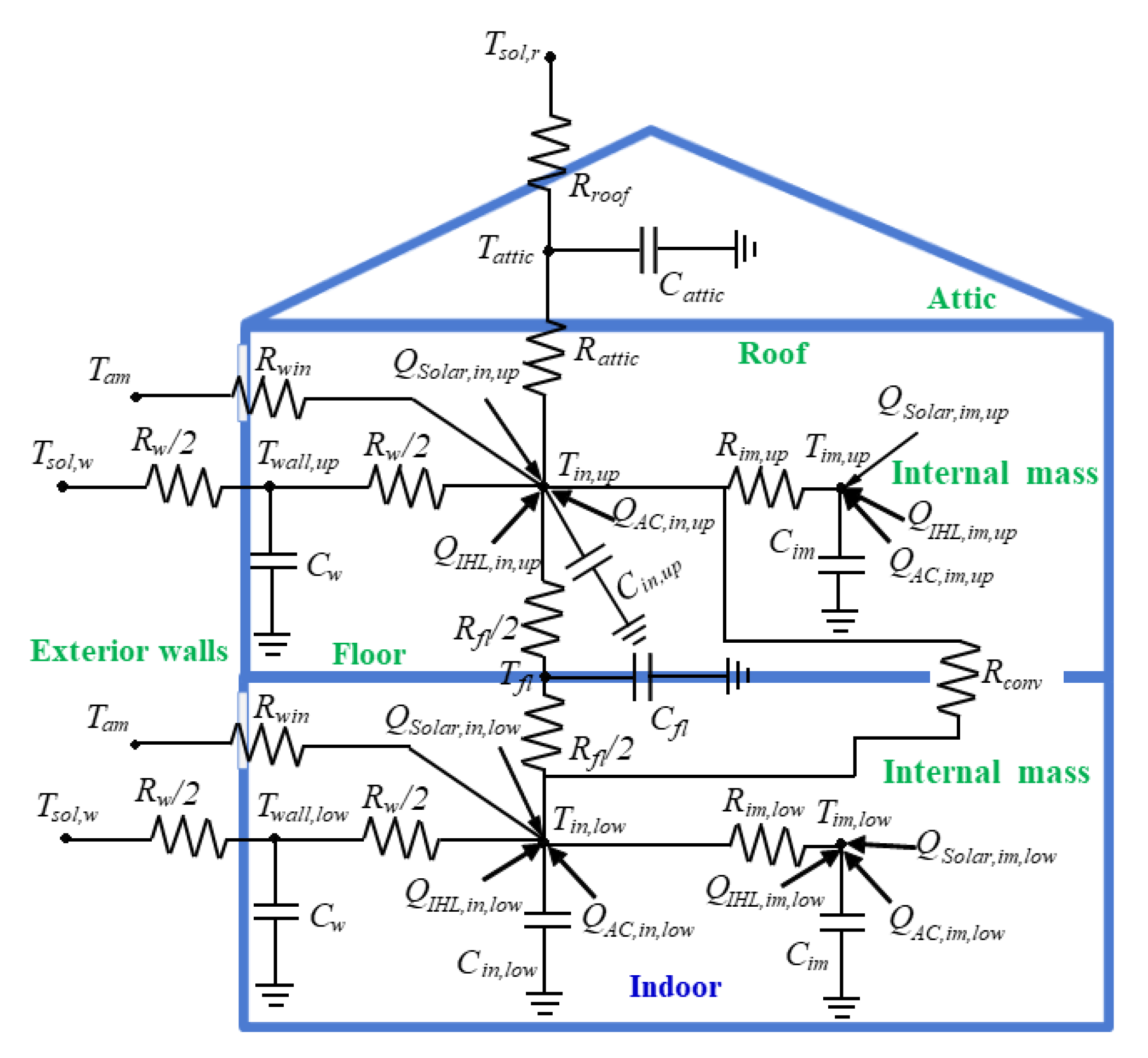
During offline training, i.e., in phase 2 (refer to Figure 1), RL agent interacts with a building simulation model. We described the development of the building simulation model in Section 3.1. We define two control steps (also described in the [18]): (1) simulation step ($\Delta t_s$) and (2) control step ($\Delta t_c$). The building simulation model simulates building’s thermal behavior for every minute, i.e., $\Delta t_s=1$ min. The RL agent interacts with the building simulation at every $\Delta t_c$ time steps ($\Delta t_c=k\Delta t_s$), observes the indoor environment, and takes appropriate action. The observations about the building’s indoor environment are modeled as a state (S) in the MDP formulation. For instance, a set of observations on the building’s indoor environment at a time instant t such as indoor temperatures and other factors such as electricity prices forms the current state of the building’s environment, i.e., $S_t$. In our case, it includes time of the day information (t), indoor temperature ($T_t^{in}$), outdoor temperature ($T_t^{out}$), and a look-ahead of electricity pricing ($P_t=\{p_t,p_{t+1},\dots ,p_{t+k},\dots \}$). Thus, the current state $S_t$ is defined as $S_t=\{t,T_t^{in},T_t^{out},P_t\}$. Similarly, the state at the previous control step is defined as $S_{t-\Delta t_c}=\{t-\Delta t_c,T_{t-\Delta t_c}^{in},T_{t-\Delta t_c}^{out},P_{t-\Delta t_c}\}$.

In this work, we used a deep Q-learning approach mentioned in [18,24] and utilized a deep Q-network (DQN), a neural network, as a function approximator. We built upon our previous work on DQN-based HVAC control for a single-zone house [30] and developed a DQN architecture for a two-zone house. There are two thermostats in the house, one for each zone, and capable of taking set point values through APIs. Since Q-learning works well for finite and discrete action space, we train DQN for ON = 1/OFF = 0 actions for both the zones and further translate the ON/OFF actions to the appropriate set point values using Equation (1), where $\Delta T$ is the small decrement factor (in case the action is ON) and increment factor (in case the action is OFF). The action = ON (‘1’) signifies the status ON for the AC, which will reduce the indoor temperature. To achieve this, we decrease the setpoint by a factor of $\Delta T$ than the current indoor temperature. In the similar fashion, the action = OFF (‘0’) signifies the RL’s intention on increasing the indoor temperature by a small amount (i.e., $\Delta T$) by turning OFF the AC. As there are two zones and two possible AC states (ON/OFF), there are total four possible actions $A=\{a_0,a_1,a_2,a_3\}$, where $a_0$ indicates OFF status for AC in both the zones which will be translated further by setting the higher set point than the current indoor temperature. The other actions can be explained in the same way as shown in

Table 1. Action space (ON = 1/OFF = 0) including both the zones. The ON/OFF actions and their equivalent set point values are shown.

Actions	AC ON/OFF Zone-1	AC ON/OFF Zone-2	Set Point-1	Set Point-2
${\mathit{a}}_{\mathbf{0}}$	0	0	$T_t^{in}+\Delta T$	$T_t^{in}+\Delta T$
${\mathit{a}}_{\mathbf{1}}$	0	1	$T_t^{in}+\Delta T$	$T_t^{in}-\Delta T$
${\mathit{a}}_{\mathbf{2}}$	1	0	$T_t^{in}-\Delta T$	$T_t^{in}+\Delta T$
${\mathit{a}}_{\mathbf{3}}$	1	1	$T_t^{in}-\Delta T$	$T_t^{in}-\Delta T$

.

$$\begin{array}{c}SetPoin{t}_t=\left\{\begin{array}{cc}{T}_t^{in}-\Delta T\hfill & \mathrm{if}actio{n}_t\equiv 1\hfill \\ T_t^{in}+\Delta T\hfill & \mathrm{if}actio{n}_t\equiv 0\hfill \end{array}\right.\end{array}$$

(1)

As discussed in the earlier paragraph, during offline training, RL agent interacts with the building simulation at every $\Delta t_c$ control interval, observes the indoor environment, and receives reward ($r_t$) as an incentive for taking the previous action, i.e., $a_{t-\Delta t_c}$. This reward is designed as a function consisting of two parts, (1) cost of performing action, i.e., $a_{t-\Delta t_c}$ and (2) comfort penalty. Equation (2) shows the reward function used in this work; it is inspired from the reward function used in the work by Wei et al. [18]. This is a negative reward function in which the reward value close to zero signifies better performance, i.e., less penalty and more negative values signifies poor action, i.e., more penalty. The first term in Equation (2) is the cost incurred due to the action taken by RL agent at time $t-\Delta t_c$. This cost is calculated as an average over the time duration $[t-\Delta t_c,t]$. The second term of the equation represents the average comfort violation over the time duration $[t-\Delta t_c,t]$. Here, $UT$ represents the cooling set point and $LT$ is some lower temperature value such that $[LT,UT]$ represents a flexibility range of temperature below the cooling set point. The RL agent would make use of this flexible temperature band to save on some costs by taking optimal actions such that the indoor temperature will always remain below the cooling set point, i.e., the homeowner’s comfort. We can provide similar arguments while the RL agent operates in the heating mode. In that case, the heating set point is used to define the $[LT,UT]$ flexibility band of temperature. In this work, we used 68 °F and 74 °F as heating and cooling set points, respectively:

$$\begin{array}{c}{r}_t=-cos{t}_{t-\Delta t_c}^{avg}-[(T_{[t-\Delta t_c,t]}^{avg}-UT)+(LT-T_{[t-\Delta t_c,t]}^{avg})]\end{array}$$

(2)

The goal of our RL agent is to learn a policy which will minimize the cost of operation and incur less or no comfort violation. More specifically, under MDP formulation, the RL agent should learn the policy (i.e., action) which will maximize not only the current reward, but also future rewards. This is represented as the total discounted accumulated reward in Equation (3) [24]. The $\gamma$ is a discount factor whose value ranges from $[0,1)$ that controls the weights of the future rewards, and T represents the time step when episode ends. The $\gamma =0$ considers only the current reward and does not take the future rewards into account. This is characterized as an RL agent being “short-sighted” by not accounting for the future benefits (rewards) and may not achieve the optimum solution. The rationale behind using future rewards is that sometimes the current low rewarded state could lead the RL agent to the high rewarded states in the future. In this work, we chose $\gamma =0.9$, which exponentially decreases the weights of the future rewards. In other words, the current reward would still get higher weight and the exponentially discounted futures rewards are taken into account as well. The higher the $\gamma$ value, the better the RL’s ability to account for the future rewards and obtain the optimal solution. The lower $\gamma$ value reduces RL’s ability to look into the future rewards which may not lead to the optimal solution.

In case of Q-learning, RL tries to learn an optimal action-value function $Q^{*}(s_t,a_t)$ which maximizes the expected future rewards (represented by Equation (3)) for action taken $a_t$ in the state $s_t$ by following policy $\pi$ i.e., ${max}_{\pi }E\left[R_t\right|s_t,a_t]$ [24]. This can be defined as a recursive function using Bellman’s equation as shown in Equation (4) [18]. The Q-learning RL algorithm estimates this optimal action-value function via iterative updates for a large number of iterations using Equation (5), where $\eta$ represents a learning rate with the range of $(0,1]$. For a large number of iterations and under an MDP environment, Equation (5) converges to the optimal $Q^{*}$ over time [18,24]:

$$\begin{array}{c}{R}_t=\sum _{t^{\prime }=t}^T{\gamma }^{t^{\prime }-t}{r}_{t^{\prime }}=r_t+\gamma r_{t+1}+{\gamma }^2{r}_{t+2}+···+{\gamma }^T{r}_{t+T}\end{array}$$

(3)

$$\begin{array}{c}{Q}^{*}(s_t,a_t)=E[r_t+\gamma \underset{a_{t+1}}{max}{Q}^{*}(s_{t+1},a_{t+1})|s_t,a_t]\end{array}$$

(4)

$$\begin{array}{c}{Q}_{t+1}(s_t,a_t)=Q_t(s_t,a_t)+\eta (r_{t+1}+\gamma \underset{a_{t+1}}{max}{Q}_t(s_{t+1},a_{t+1})-Q_t(s_t,a_t))\end{array}$$

(5)

The iterative Q-learning strategy of Equation (5) uses a tabular method to store state-action Q values. This method works well with the discrete state-action space and quickly becomes intractable for a large state-action space. For instance, in our case, the indoor temperature and outdoor temperature are the continuous quantities that make infinite state-action space. This is where DQN is useful that uses a neural network as a functional approximator to approximate the state-action value $Q(·)$. Algorithm 1 represents the deep Q-learning procedure used in this work, which is inspired from Wei et al. [18] and Mnih et al. [24]. This approach uses the DQN neural network structure as shown in Figure 5. Mnih et al. [24] implemented a Q-learning strategy using deep Q-networks (DQN), that uses two neural networks and experience replay. The first network Q is called the “evaluation network”, and the second network $\widehat{Q}$ is called a “target network” (refer to Figure 5). Equation (5) needs two Q values to be computed. The first is $Q_t(s_t,a_t)$: the Q-value of the action $a_t$ in the current state $s_t$, and the second is $Q_t(s_{t+1},a_{t+1})$: to calculate the maximum of the Q-values of the next state $s_{t+1}$. The evaluation network (Q) is used to evaluate $Q_t$ using one forward pass with $s_t$ as an input. The term “($r_{t+1}+\gamma \underset{a_{t+1}}{max}{Q}_t(s_{t+1},a_{t+1})$” represents a “target” Q-value that RL-agent should learn. If we use the same network to compute both Q-values i.e., $Q_t(s_t,a_t)$ and $Q_t(s_{t+1},a_{t+1})$ makes the target unstable due the frequent updates made in the evaluation network. To avoid this, Mnih et al. suggested using two separate neural networks such that the evaluation network performs frequent updates in the network and copies updated weights to the target network after certain updates. Thus, the target network updates itself slowly compared to the evaluation network, which improves the stability of the learning process.

The training starts by initializing weights of both the networks (i.e., Q and $\widehat{Q}$) randomly, reserving the experience replay buffer ($MB$) and initializing other necessary variables (lines 1–12 in Algorithm 1). We train the RL agent for multiple episodes where each episode consists of multiple training days (e.g., two months of summer). In the beginning of each episode, we reset the building environment of the simulator, get the initial observation ($S_{pre}$) from the building environment, and randomly choose some initial action (refer to lines 15–18 in Algorithm 1). The lines 19–38 of the algorithm represent a loop where the building simulation model simulates the thermal behavior of the building at each $t_s$ time step. If the current time step $t_s$ is a control step, i.e., $t_{s}mod\Delta t_c=0$, then we fetch the current state of the building’s indoor environment ($S_{curr}$) and calculate the reward (r) as a response of the action taken at the previous control step (refer to lines 21–22 in Algorithm 1). Furthermore, we store the tuple $<S_{pre},a,r,S_{curr}>$ to the experience replay memory ($MB$) (refer line 23). Next, a mini-batch of tuples is randomly chosen from this replay memory and used for the mini-batch update (described on lines 24–25 of Algorithm 1), and if it’s time to update the target network, then copy the weights of the evaluation network to the target network (refer to line 26). Lines 26–32 choose action using a decaying $ϵ$-greedy strategy. In the beginning, the RL agent explores random actions with high probability (line 28), whereas, as training progresses, the probability of exploitation increases, and the RL-agent uses the learned actions more than choosing random actions (line 30). Line 36 continues executing the earlier action if the current time step is not a control step.

Algorithm 1 Neural network-based Q-learning.

1: Env ← Setup simulated building environment  2: MB ← Experience Replay Buffer  3: Δts ← Simulation time step (here, 1 min)  4: Δtc ← k × Δts RL’s control step interval (here, k = 15)  5: NDays ← Number of operating days for training  6: Nepisodes ← Number of training episodes  7: TSmax ← NDays × 24 × (60/Δts)  8: nbatch ← minibatchsize  9: ϵ ← initial exploration rate 10: Δϵ ← exploration rate decay 11: Q(s, a; θ)←Initialize(Q, θ) 12: $\widehat{Q}(s,a;\widehat{\theta })$ ← Initialize($\widehat{Q},\widehat{\theta }$) 13:   14: forepisode = 1 to Nepisodes do 15:  Env← ResetBuildingSimulation(Env) 16:  Spre ← ObserveBuildingState(Env, 0) 17:  a ← GetInitialAction(Env) 18:  Set points ← ConvertActionToSetpoints(Spre, a) 19:  for ts = 1 to TSmax do 20:   if ts mod Δtc = 0 then 21:    Scurr ← ObserveBuildingState(Env, ts) 22:    r ← CalReward(Env, Spre, a, Scurr) 23:    AppendTransition(MB, 〈Spre, a, r, Scurr〉) 24:    [T] ← DrawRandomMiniBatch(MB, nbatch) 25:    TrainQNetwork(Q(·;θ),[T]) 26:    if time to update target: $\widehat{Q}(·;\widehat{\theta })\leftarrow Q(·;\theta )$ 27:    if GenerateRandomNumber([0, 1]) < ϵ then 28:     a ← ChooseRandomAction([a0, a1, a2, a3]) 29:    else 30:      $a\leftarrow arg\underset{a^{\prime }}{max}Q(S_{curr},a^{\prime };\theta )$ 31:    end if 32:    $ϵ\leftarrow ϵ-\Delta ϵ$ 33:    Setpoints ← ConvertActionToSetpoints(Scurr, a) 34:    Spre ← Scurr 35:   end if 36:   SimulateBuilding(Env, ts, Setpoints) 37:  end for 38: end for

3.4. Feature Scaling

The values of the state features such as time of the day (t), indoor temperature ($T^{in}$), outdoor temperature ($T^{out}$), and electricity pricing of the input state vector, i.e., $S_{pre}$ and $S_{curr}$ varies significantly. For instance, in our dataset, the indoor temperature varies between [70 °F, 74 °F], the outdoor temperature in Knoxville, TN, USA during summer varies between [50 °F, 90 °F], and the values of electricity prices in our dataset vary between [0.25 $, 0.5 $]. As a data pre-processing step, before training, we scale the features to the range [0, 1] using minimum and maximum values of each feature. For indoor temperature, we use the cooling setpoint set by the user, i.e., $UT$ and $LT=UT-2$ (a 2° flexibility band below $UT$) as a range to scale the indoor temperature. We believe that this way of scaling the indoor temperature will help the RL agent to adapt to any comfort range. We performed few experiments to validate this behavior and the results are presented in Section 4.

4. Experiments and Results

In this section, we start with the description of the dataset used in this work. Furthermore, we present various results on performance of the simulation model and the RL model in the simulated environment as well as in the real house.

4.1. Dataset Used

The following list presents the dataset used in this work to build the simulation model and RL training.

• Weather data: The building model requires weather-related data, including ambient temperature, direct normal irradiance, diffuse horizontal irradiance and wind speed. For the building model training process, the ambient temperature used was measured locally at the house with a data logger, while the other values were pulled from a nearby weather station. During the RL training process, these data were taken from Typical Meteorological Year data for Knoxville, TN, USA [31]. This source provides hourly resolution data for a year and is meant to represent typical weather of a location. Linear interpolation was used to generate minute-level data from the hourly TMY data.
• Price data: The price data used for this study includes two distinct price levels, representing peak price and off-peak price that are common in time-of-use (TOU) electricity rate plans. Unlike typical TOU plans that may only have one peak price period, the price schedule used in this study has multiple peak price periods of three-hour duration separated by three hours of non-peak price. This was done to increase the learning rate of the RL model during the pre-training by providing eight price change events per day instead of only two.

4.2. Validation of the Trained Building Model

The unknown model parameters of the building simulation model were trained on measured data from the house using a particle swarm optimization algorithm to identify the values of the parameters that minimized the sum of the root mean squared error (RMSE) of the upstairs and downstairs air temperatures. At the time of model development, there was no access to logged indoor temperature data from the thermostats. In place of the thermostats’ measured temperatures, measurements from temperature sensors located next to the thermostats and collected on the house data logging system were used instead. The trained parameters were validated on a separate set of data spanning approximately eight days with the resulting performance shown in Figure 6. The validation of the simulated zone 1 indoor temperature showed an RMSE value of 0.57 °C (top figure in Figure 6) and zone 2 indoor temperature showed the RMSE of 0.56 °C (top figure in Figure 6), which is reasonably good.

4.3. Training Performance of the RL Model (Phase 2)

We used weather data for the months of June and July and performed training for 50 episodes.

Table 2. Various DQN related parameters and their values used during the training.

Parameter	Value
Episodes	50
Simulation step ($\Delta t_s$)	1 min
Control step ($\Delta t_c$)	15 min
Learning rate	0.001
Optimizer	Adam
Reward decay ($\gamma$)	0.9
$ϵ$-greedy value	0.99
Target replacement iterations	200
Initial steps	1440
Batch size	32
Experience replay memory size	20,000
[Heating set point, Cooling set point]	[68 °F, 74 °F]
[LT, UT]	[72 °F, 74 °F]

summarizes the training setup. As mentioned in Section 3.3, the simulation step ($\Delta t_s$) and the control step ($\Delta t_c$) were set to 1 min and 15 min, respectively. The reward decay ($\gamma$) was set to 0.9 which controls the decay of the future rewards. The exploration (or exploitation) rate was controlled by the $ϵ$-greedy value, which was initially set to 0.99. During training, initially, an RL-agent chose actions randomly with the 0.99 probability, i.e., exploration. As training progressed, this value decreased until it reached a minimum $ϵ$ value of 0.05. We decreased the $ϵ$ value exponentially as training progresses. This way, the initial exploration rate decreased, and the RL agent exploited its learning more. The evaluation network’s weights were copied to the target network after every 200 training iterations. We used 1440 min (one day) as initial steps during which we allowed an RL-agent to observe the environment and execute the random action. This was to make sure that a sufficient number of tuples existed in the experience replay memory before training began. The size of the experience replay memory was set to 20 K. At every learning step, the RL-agent extracted a batch of 32 tuples randomly from the experience replay memory. We used Adam optimizer [32] with a learning rate of 0.001. For this work, we used a fixed schedule [heating setpoint = 68 °F, cooling setpoint = 74 °F] and the flexibility band of 2 °F, i.e., [72 °F, 74 °F].

During the training phase, i.e., phase 1, we observed the convergence of the reward, overall cost of the HVAC operation, and comfort violation over the training iterations. We repeated the training process with various values of the parameters mentioned in Table 2 until we obtained the satisfactory performance. Here, we present the training performance of the RL model which showed the satisfactory performance and discuss its convergence. Figure 7 shows three plots showing the training efficiency in terms of reward (Figure 7a), cost of HVAC operation (Figure 7b), and minutes outside comfort (MOC) (Figure 7c). As mentioned earlier, we repeated the training for 50 episodes where every episode had 61 days. During training, we collected the average reward per episode, total cost of HVAC operation for an episode, and total minutes for which the indoor temperature in both the zones were out of the range comfort (MOC) (i.e., above cooling setpoint+AC’s dead band value) for an episode. We repeated the training procedure five times, every time with different seed values for the random initialization of the neural network parameters. In this way, for each episode, we collected five values for average reward per episode, total cost, and total MOC.

We used values from 50 episodes and generated three graphs showing the training progress and its efficiency (refer to Figure 7). The shaded portion in the figure depicts the min-max range, and the dashed line represents the mean value of the respective quantity, i.e., average reward, cost, and MOC. Figure 7a shows the convergence of the reward, starting with high negative value and reaching towards zero as training progresses, which is expected behavior when using a negative reward strategy. However, we observed less variations in the five reward values for each episode. Similarly, Figure 7b shows the variations in the episodic cost of the HVAC operation. We can see that, during the initial few episodes, the cost was high; however, the cost reduced as the training progressed. Similar observations can be made from Figure 7c, which shows the reduction in the total minutes of comfort violation as training progressed. In summary, we observed the convergence in the training of the RL model for controlling HVAC in cooling mode. We also noticed that the training converged roughly during the 25th episode which is called early convergence. In the future, we intend to perform more experiments to understand this behavior. Furthermore, we used this trained RL model to validate its performance (i.e., phase 2 and phase 3) in different environments which were not present during the training process (i.e., phase 1).

4.4. Validation of the Trained RL Model (Phases 2–3)

After we observed the convergence in the training performance of the model, we validated the pre-trained model with the environment that was not used during training. We developed a separate environment to validate the pre-trained RL model and its performance in the different synthetic houses with varying conditions. This environment facilitates ways to deploy the pre-trained models virtually in the building before deploying them to the real houses. We used a fixed setpoint (cooling) thermostat logic as a baseline to compare the performance of the RL model in terms of the cost savings.

We validated the pre-trained model in two phases (phases 2 and 3). In phase 2, we validated the pre-trained model using the same building simulation model which was used during training (i.e., same house); however, we used a different month’s weather data. Since we trained the model using weather data from June and July, we validated it using weather data for August. Once we were satisfied with the pre-trained model’s performance in phase 2, we further validated its performance using various synthetic houses which is phase 3. The process of generating synthetic houses is explained in Section 3.2.

4.4.1. Validation with the Same House as a Simulation

We used the trained building model that was used during the training phase for simulating the building’s thermal response with the pre-trained RL model for the August data. We carried out this virtual deployment for three different cooling setpoints, i.e., 73 °F, 74 °F and 75 °F. For each cooling setpoint, RL tries to utilize 2 °F of flexibility band below the cooling setpoint to automatically adjust the setpoint. The first three columns of

Table 3. Comparison of the cost of operation, energy consumption and MOC for a fixed cooling set point baseline and pre-trained RL model in the validation of phase 2.

Cooling Set Point →		73 °F	74 °F	75 °F	(74, 75, 73) °F
Baseline	Energy (kWh)	368.01	333.49	301.37	334.84
	Cost ($)	56.94	51.91	46.74	51.69
	MOC (min)	0	0	0	97
RL	Energy (kWh)	430.89	390.96	352.72	393.97
	Cost ($)	40.10	35.46	31.58	36.09
	MOC (min)	0	0	0	79
% Cost reduction		29.57%	31.68%	32.43%	30.17%

shows the cost incurred and energy used by simulating both baseline and the pre-trained RL model for the month of August with these fixed cooling setpoints. We also validated the performance of the pre-trained model with a variable schedule. This setup is represented by the fourth column of Table 3. In this setup, we assumed a scenario where the homeowner set the cooling setpoint as 74 °F for the first 10 days, 75 °F for the next 10 days, and 73 °F for the remaining days of the month of August. For all four cases, we observed ≈30% cost reduction over baseline when using the pre-trained RL model (as shown by the bottom row in Table 3).

For the purpose of visualization, we present the temperature variations graph for the variable setpoint scenario (i.e., fourth column of Table 3) both using the pre-trained model and the fixed cooling setpoint. Figure 8 shows two plots out of which the first plot (Figure 8a) shows the indoor temperature variations for the fixed cooling setpoint and the second plot (Figure 8b) shows the indoor temperature variations due to the decisions made by the pre-trained RL model. This validation experiment represents a scenario of a variable schedule where, for the first ten days, the homeowner sets the cooling setpoint to 74 °F, for next ten days increased to 75 °F, and for the remaining 11 days reduced down to 73 °F. The difference between the fixed cooling point baseline and the RL operations is that the baseline uses the cooling setpoint to control the HVAC operation, whereas the RL model uses a 2 °F of flexibility range below the cooling setpoint to operate the HVAC such that the price of operation is lower than the baseline while satisfying the homeowner’s comfort. The logic behind this operation is explained in Section 3.3. It must be noted that a larger flexibility range (e.g., >2 °F) would provide greater opportunity for pre-cooling and therefore greater cost savings potential. Similarly, a smaller flexibility range (e.g., <2 °F) would not provide much opportunity on to RL for cost saving.

The green lines represent the lower and upper threshold of the 2 °F of flexibility range below the cooling setpoint. The plots in Figure 8 show temperature variations and the AC status (cool on) for both zones. The color blue represents zone 1 and red represents zone 2. Additionally, the plots show outdoor temperature and price signal. We have scaled the price signal for the visualization purpose. The actual values of the price are $\$0.05$ for low price timings and $\$0.25$ for high price timings. It can be seen in Figure 8a that the baseline operation tried to maintain the indoor temperature around the cooling setpoints by performing ON/OFF operations of AC. However, the pre-trained RL model took advantage of the 2 °F of flexibility range to vary the cooling setpoint such that it saved some money while maintaining the home owner’s comfort (refer to Figure 8b). Here, the price ratio of the high price to low price is five. Since RL is taking the advantage of the lower price as well as the 2 °F of flexibility range to achieve cost savings, a smaller price ratio would result in lower cost savings. Similarly, a larger price ratio would result in higher cost savings.

The shaded regions represent a hypothetical scenario of modifying the cooling setpoint. The first time the cooling setpoint was changed from 74 °F to 75 °F, and second time the setpoint was changed from 75 °F to 73 °F. Both the operations, with the fixed setpoint baseline and with the pre-trained RL model, showed the adaptability to the changes in the setpoint values. In case of the baseline, it is quite natural because of its rule-based nature. However, the RL model does not embed any such rule. It was able to adapt to the changing setpoint because of the feature scaling logic we used. In this logic, we scaled down the indoor temperature to the range of $[0, 1]$ by using schedule_LT and schedule_UT as the min-max of the range. This trick of feature scaling removes the dependency on the absolute value of the indoor temperature in the state variable which helps in adapting the changes in the setpoints.

Figure 9 shows the daily cost comparison of the baseline operation and the pre-trained RL model operation for controlling HVAC in the cooling mode. From the graph, it is clear that the RL is saving some money all the days during a month of operation. We observed that the RL-based HVAC control saved ≈25%–30% money per day. This can be seen in Table 3. We also observed that the RL’s operation consumed more energy as compared to the baseline which is consistent for all four setups (refer to Table 3). Moreover, we observed some comfort violations of 97 min for baseline and 79 min for RL-based operation in the fourth setup where we used a variable schedule. For the other three cases, in which we used fixed setpoint throughout the operation, no comfort violation was observed (i.e., MOC = 0).

To understand the reasoning behind, (1) RL’s cost saving over the fixed cooling setpoint baseline, (2) RL’s extra energy consumption compared to the baseline operation, and (3) the comfort violations during the variable setpoint setting, we present Figure 10, which zooms into the second shaded region of the Figure 8, where the setpoint was changed from 75 °F to 73 °F. Figure 10a shows the zoomed in view of the baseline plot shown by Figure 8a, and Figure 10b shows the zoomed in view of the plot showing RL’s operation in Figure 8b. We observed that the pre-trained RL model tried to cool down the zones more during the low price timings and tried to minimize cooling during high price timings. This can be observed by comparing the AC status shown by cooling on lines and the price signal in Figure 10b. We highlighted these events as “pre-cooling” as shown in the figure. In contrast, the fixed setpoint baseline performed cooling whenever the indoor temperature was above the cooling setpoint without taking into consideration the pricing information (refer to Figure 10a). This is the reason behind RL’s cost reduction as compared to the fixed cooling setpoint baseline. Furthermore, it can be observed that RL maintains the house at a lower temperature on average compared to the baseline. This results in a larger cooling load on the HVAC system due to increased heat gains through the envelope caused by a larger temperature differential between the indoor and outdoor air. This explains why pre-trained RL model based HVAC control consumed more energy than the baseline as shown in Table 3. This can also be justified by the reward function used for training the RL model (shown in Equation (2)), which uses only cost of operation to penalize the RL-agent. In Figure 10a,b, the region marked as “comfort violation” is where the indoor temperature violated the cooling setpoint. This is the reason behind the MOC values of 79 and 97 min for the RL and baseline’s operation, respectively. We calculated MOC as the sum of the number of minutes the indoor temperature was above the cooling setpoint+the AC’s dead band. It can be seen in Figure 10 that both the baseline and RL control tried to set the cooling setpoint with respect to the changed cooling setpoint (i.e., from 75 °F to 73 °F); however, indoor temperature took some time to cool down, which was reflected as MOC as shown in Table 3 and comfort violation as shown in Figure 10. In the case of baseline, this can not be avoided; however, the RL-agent can use some schedule look ahead to respond to such events by pre-cooling to avoid the comfort violations.

We observed similar validation performances for the other three settings shown by the first three columns of Table 3. Due to the space constraints and to avoid repetition, we are not providing the temperature variation and daily cost comparison plots in the main text. Therefore, in this section, we provided only the plots of temperature variations and daily cost comparison for the fourth setting in which we used all other three cooling setpoints, i.e., 73 °F, 74 °F, and 75 °F to create a scenario with the variable schedule.

4.4.2. Validations Using Synthetic Houses

After we observed a satisfactory performance during the validation of the pre-trained model in phase-2, we further validated the performance of the pre-trained RL model with the synthetic houses to examine the adaptability and scalability of the pre-trained RL model in the different house settings. As described in Section 3.2, we developed a few synthetic houses by varying the building parameters of the original building simulation model. In this experiment, we chose two synthetic houses randomly and used a pre-trained model to perform HVAC control with four settings described in Table 3.

Table 4. Comparison of the cost of operation, energy consumption, and MOC for a fixed cooling set point baseline and pre-trained RL model in the validation of phase 2 with the synthetic House 1.

Cooling Set Point →		73 °F	74 °F	75 °F	(74, 75, 73) °F
Baseline	Energy (kWh)	330.15	297.72	269.20	299.61
	Cost ($)	50.94	46.00	41.81	45.98
	MOC (min)	0	0	0	97
RL	Energy (kWh)	390.75	352.36	317.71	358.73
	Cost ($)	35.17	30.94	27.41	31.57
	MOC (min)	0	0	0	69
% Cost reduction		30.9%	32.72%	34.44%	31.33%

shows the cost, energy, and MOC comparison of the fixed cooling setpoint and pre-trained RL model based HVAC control in the synthetic house 1 and

Table 5. Comparison of the cost of operation, energy consumption, and MOC for a fixed cooling set point baseline and pre-trained RL model in the validation of phase 2 with the synthetic House 2.

Cooling Set Point →		73 °F	74 °F	75 °F	(74, 75, 73) °F
Baseline	Energy (kWh)	287.44	266.22	244.63	268.00
	Cost ($)	44.01	40.42	37.46	40.87
	MOC (min)	0	0	0	68
RL	Energy (kWh)	329.30	295.23	265.59	299.62
	Cost ($)	30.25	26.55	23.42	26.74
	MOC (min)	0	0	0	59
% Cost reduction		31.26%	34.31%	37.47%	34.57%

shows similar results for synthetic house 2. The difference in the energy consumption of baseline and RL operations with synthetic houses (shown in Table 4 and Table 5) with the energy consumption of the baseline and RL operation with the original building simulation model (shown in Table 3) is an indicator of the variations in the thermal behavior of the developed synthetic houses. We observed that the pre-trained RL model achieved roughly 30–35% of cost reduction as compared to the fixed cooling setpoint baseline. These results are consistent with the validation performance of the pre-trained model presented in the earlier Section 4.4.1. This provides experimental evidence that the pre-trained RL model has the potential to adapt to the different house environment which was not present during the training phase. Refer to Appendix A for the temperature variations and daily cost comparison plots of the validation experiments performed with synthetic houses. Figure A1, Figure A2 and Figure A3 show the plots for the temperature variation, a zoomed in view of the period where the cooling setpoint was changed and the daily cost comparison, respectively, for the validation experiment with synthetic house 1. Similarly, Figure A4, Figure A5 and Figure A6 show the plots for the temperature variation, a zoomed in view of the period where the cooling setpoint was changed, and the daily cost comparison respectively for the validation experiment with synthetic house 2.

We performed the validation experiments (phases 2 and 3) with fixed and variable cooling setpoint, and with different synthetic houses. These validation results showed the satisfactory performance on scalability and adaptability of the developed pre-trained RL model in different environment and varying house settings.

4.5. Performance in the Real House (Phase 4)

After validating the performance in simulations (phases 2–3), we deployed the RL at the research house described in Section 3.1. In the first deployment, the RL was pre-trained using the building model parameters that were identified for that house. In the second deployment, the RL was pre-trained on one of the synthetic house’s building parameters to evaluate the robustness of the pre-training process. In order to estimate the savings potential of RL, we need to compare the energy cost during RL operation with a baseline. A fixed cooling setpoint baseline was chosen with a cooling setpoint at the upper limit of the comfort range used by the RL. Since the building model parameters were developed using indoor temperature measured by sensors rather than the actual thermostats, an initial re-calibration of the model was performed to improve the model accuracy. The improved building model was then used to simulate the baseline case and create a reference for evaluating the cost savings of the RL.

4.5.1. Building Model Re-Calibration

In order to improve the accuracy of the building model for the baseline simulation, the model was re-calibrated using data from the first RL deployment. The building model was originally trained and calibrated using temperature data collected by data logger sensors. While this is generally representative of the building thermal response, it is not identical to the temperature measurement used by the thermostat for controlling the HVAC system. Therefore, the main purpose of the re-calibration is to better ensure that the response and trend of the building model indoor temperatures matches that of the temperatures measured by the thermostats. This is critical for ensuring the HVAC system cycling in the model is consistent with the actual system. During the RL deployment, the thermostat temperatures and setpoints were recorded at 15 min intervals. The recorded RL setpoints were then fed into the simulation along with the measured weather data for each day. In this way, we can compare the measured temperatures, HVAC energy consumption, and energy costs to those that are simulated to gauge the accuracy of the building and HVAC system models. Based on these results, the building parameters were manually tuned to improve the accuracy of the models.

4.5.2. Baseline Simulation

With the building model re-calibrated to better match the thermal response of the building, we can now use the model to simulate baseline performance. The baseline case uses a fixed cooling setpoint at 74 °F, the upper end of the comfort range. This assumes that homeowners will generally set their thermostat to the upper edge of their comfort range in order to minimize energy use. With this baseline case, any savings achieved by RL can be contributed to “pre-cooling” during low price periods and not running the home at a higher indoor temperature than the baseline. Since the building model includes unknown temperatures (e.g., indoor mass and internal wall temperatures), and there is no measured data to calibrate these values on for the baseline case, the baseline simulations were run for 30 days. The first 29 days of the baseline simulation are used as a “warm-up” period to allow the unknown temperatures to settle to realistic values. The warm-up period was confirmed to be sufficiently long by checking convergence of the results (i.e., the results when using 27-day, 28-day, and 29-day warm-up periods were identical). All unknown temperatures are initialized to the cooling setpoint at the beginning of the warm-up period. The 30 days are simulated using the fixed cooling setpoint and the data from the final day is used for the analysis.

4.5.3. RL Deployed with Model Pre-Trained on the Deployed House Data

During the first deployment, the RL model was pre-trained using the building parameters trained on the research house data. The measured data during the deployment was used to re-calibrate the building model as described in Section 4.5.1, and the re-calibrated model was used to simulate the baseline case as described in Section 4.5.2. The re-calibrated building model simulation with RL setpoints and the fixed baseline simulation are shown for three days of deployment in Figure 11, Figure 12, Figure 13, Figure 14, Figure 15 and Figure 16. Results are summarized in

Table 6. HVAC cost savings calculations for first deployment.

Date →		19 June 2020	23 June 2020	24 June 2020
Baseline	Simulated cost ($)	0.87	1.22	1.34
	Simulated energy (Wh)	6160	8178	8770
RL	Simulated cost ($)	0.72	1.14	1.17
	Measured cost ($)	0.72	1.03	1.24
	Simulated energy (Wh)	6956	8055	9343
	Measured energy (Wh)	6447	7790	9046
% Cost reduction	RL simulation	17%	7%	13%
	RL measured	17%	16%	7%

. RL savings were calculated by comparing both the measured data during the RL deployment and the simulated data with RL setpoints to the baseline simulations. RL savings were estimated at 7–17% for this deployment. These savings are slightly less than those simulated during the RL training process (i.e., in phases 2 and 3). We believe that there are likely two factors contributing to this difference. First, as can be seen in the re-calibrated model simulations plots (Figure 11, Figure 13 and Figure 15), the temperature measured by the data acquisition system (DAQ) has significantly higher magnitude fluctuations than the thermostat (Tstat) measured temperatures. Since the building model was trained using the DAQ measured temperatures, the thermal response that the RL is expecting is quite different from what it was trained on. Second, since the RL was only dispatching new setpoints every 15 min, there are time intervals where the HVAC system is cycling. Ideally, the system would stay either on or off, depending on the RL decision, for the entire 15 min interval. These issues can likely be resolved by a combination of the following: (1) re-training the building model using the thermostat-measured temperatures as the inputs, (2) increasing the magnitdue of the setpoint change by RL to better ensure that the HVAC system maintains the desired on/off status for the entire 15 min interval, or (3) reducing the decision timestep of the RL to 5 min. instead of 15 min.

4.5.4. RL Deployed with Model Pre-Trained on Synthetic House Data

During the second deployment, the RL model was pre-trained using one of the synthetic house building parameters. This was done to test whether RL could be pre-trained on a generic building model and deployed in many different houses with positive results. Figure 17, Figure 18, Figure 19 and Figure 20 show the re-calibrated model simulation and baseline simulation compared to the measured data. Results are summarized in

Table 7. HVAC cost savings calculations for second deployment

Date →		08 July 2020	09 July 2020
Baseline	Simulated cost ($)	2.13	2.40
	Simulated energy (kWh)	14.7	15.5
RL	Simulated cost ($)	1.68	2.00
	Measured cost ($)	1.82	2.14
	Simulated energy (kWh)	15.3	16.1
	Measured energy (kWh)	14.6	15.8
% Cost reduction	RL simulation	21%	17%
	RL measured	15%	11%

. The RL savings range from 11–21%, similar to the results from the first deployment. This is evidence that RL can be pre-trained on a model that does not exactly match the building that it is deployed on. This is further supported by the first deployment, since the original building model that RL was pre-trained on used a different temperature sensor with different thermal response.

5. Conclusions

In this paper, we presented an end-to-end workflow for evaluating the adaptability of the reinforcement learning (pre-trained) based HVAC control for residential houses. The pre-trained RL model developed in the simulated environment showed around 30 $ of energy cost savings with much less comfort violation when validated in the virtual deployment mode. This provided us with experimental evidence that the RL agent was able to take advantage of the low price period and the strategy of 2 °F flexibility band to save the energy cost while maintaining the user’s comfort. The similar strategy can be utilized while training the RL model for winter where the heating setpoint can be used as $LT$ and a 2 °F flexibility range above $LT$, i.e., $UT=LT+2$ to allow RL to pre-heat during low price periods to save cost. However, the experiments are required to evaluate the performance with the 2 °F flexibility range. We also performed validation using synthetic houses in the virtual deployment mode where the cooling setpoint ($UT$) varied at ≈10 days of interval for a month of August. Along with the energy price savings, we found that the pre-trained RL model was able to adapt to the environment of the synthetic houses as well as the changing cooling setpoint. The adaptability to changing comfort range was achieved using the feature scaling strategy that uses [$LT(=UT-2$), $UT$] and flexibility range to scale the indoor temperature features of the state. Here, we found some comfort violation when setpoint changed from 75 °F to 73 °F. We believe that if we provide some look-ahead information on the changing setpoint the RL agent could pre-cool more and quickly adapt to the new setpoint.

After we obtained the satisfactory performance in the virtual deployment mode, i.e., in phase 2 and 3, we deployed the pre-trained model in the real house. Results from both RL deployments indicated RL savings in the range of 11–21% for different days. This is lower than the RL savings that were estimated during the RL training process but still very encouraging. Some factors that are likely contributing to this difference is the different thermal response of the temperature sensor used to pre-train the RL compared to the actual thermostat temperature sensor coupled with the 15 min timestep used by RL. This resulted in the HVAC cycling on, during some time periods, when RL was expecting the system to be turned off, typically during peak price periods, resulting in higher than expected costs for RL. This could be mitigated by either setting the cooling setpoint higher when RL decides the system should be off, ensuring it stay off the entire 15 min, or by using a timestep shorter than 15 min. Retraining the building model using the thermostat temperature measurement would also help reduce these instances. RL performed similarly well in both deployments, which illustrates its ability to save on costs even when pre-trained on different building models.

It should be noted that the cost savings potential of pre-cooling during low price periods, as displayed by RL, is dependent on several factors including the price signal, the allowable comfort range (flexibility range for RL), the weather, and the building’s thermal characteristics. This study used a specific set of inputs to evaluate RL, and the resulting savings are specific to these inputs. This study used a very dynamic price signal with many price changes over the course of the day. It is expected that a dynamic price signal will increase the cost savings potential by providing more opportunities for pre-cooling when compared to a price signal with fewer price changes. Additionally, the price ratio of the high price to low price was five. A smaller price ratio would result in lower cost savings, and a larger price ratio would result in higher cost savings. The allowable flexibility range provided to the RL for the indoor temperature was limited to 1.1 °C (2.0 °F). A larger flexibility range would provide greater opportunity for pre-cooling and therefore greater cost savings potential. Similarly, a smaller flexibility range would not provide much opportunity for cost saving. The combination of weather and building characteristics defines the building cooling load. The HVAC size relative to the cooling load will determine the ability of the HVAC system to pre-cool the building. Systems that are undersized will not be able to pre-cool the building and therefore will not be able to achieve any cost savings associated with pre-cooling during low price periods. Additionally, buildings with more thermal mass will have longer periods of time that pre-cooling will be effective and will also extend the duration that the home can “coast” through high price periods without needing cooling.

There are several items that we plan to investigate in future work including:

• Increasing the temperature setpoint change that RL dispatches for on/off decisions to help ensure the HVAC system stays on or off for the entire timestep.
• Testing timestep intervals shorter than 15 m.
• Evaluating the performance of online learning. Determine if it can increase savings for the case when RL is pre-trained on a model that does not match the actual building. Evaluate how long this process takes.
• Evaluating how the price signal used in pre-training affects the ability of RL to work with different price signals when deployed.
• Perform experiments to quantify the impacts of the varying flexibility ranges as well as different price signals with varying high to low price ratio on RL’s ability to reduce cost.

This work provides a systematic treatment on developing the RL based techniques for optimal HVAC control and its practical utility and challenges in the real-world scenarios. It demonstrates that pre-trained RL can achieve HVAC cost savings even when it is deployed in a house that does not match the building model used during the pre-training. We believe that the approach provided in this paper would benefit further development and research in the field of building energy optimization using reinforcement learning techniques.

References

1. Shaikh, P.H.; Nor, N.B.M.; Nallagownden, P.; Elamvazuthi, I.; Ibrahim, T. A review on optimized control systems for building energy and comfort management of smart sustainable buildings. Renew. Sustain. Energy Rev. 2014, 34, 409–429. [Google Scholar] [CrossRef]
2. US-EIA. Use of Energy Explained Energy Use in Homes. Available online: https://www.eia.gov/energyexplained/use-of-energy/homes.php (accessed on 31 August 2020).
3. Zandi, H.; Kuruganti, T.; Vineyard, E.; Fugate, D. Home Energy Management Systems: An Overview. In Proceedings of the 9th International Conference on Energy Efficiency in Domestic Appliances and Lighting (EEDAL2017), Irvine, CA, USA, 13–15 September 2017; Bertoldi, P., Ed.; Publications Office of the European Union: Luxembourg, 2017; Number 217, pp. 606–614. [Google Scholar]
4. Batchu, R.; Pindoriya, N.M. Residential Demand Response Algorithms: State-of-the-Art, Key Issues and Challenges. In Proceedings of the 7th International Conference, WiSATS 2015, Bradford, UK, 6–7 July 2015; Pillai, P., Hu, Y.F., Otung, I., Giambene, G., Eds.; Springer International Publishing: Cham, Switzerland, 2015; pp. 18–32. [Google Scholar] [CrossRef]
5. Afram, A.; Janabi-Sharifi, F. Theory and applications of HVAC control systems—A review of model predictive control (MPC). Build. Environ. 2014, 72, 343–355. [Google Scholar] [CrossRef]
6. Karray, F.; De Silva, C. Soft Computing and Intelligent Systems Design: Theory, Tools, and Applications, 1st ed.; Addison-Wesley: Boston, MA, USA, 2004. [Google Scholar]
7. Ahmed, O. Method and Apparatus for Determining a Thermal Setpoint in a HVAC System. U.S. Patent 6,145,751, 14 November 2000. [Google Scholar]
8. Gouda, M.; Danaher, S.; Underwood, C. Thermal comfort based fuzzy logic controller. Build. Serv. Eng. Res. Technol. 2001, 22, 237–253. [Google Scholar] [CrossRef]
9. Kolokotsa, D.; Tsiavos, D.; Stavrakakis, G.; Kalaitzakis, K.; Antonidakis, E. Advanced fuzzy logic controllers design and evaluation for buildings’ occupants thermal–visual comfort and indoor air quality satisfaction. Energy Build. 2001, 33, 531–543. [Google Scholar] [CrossRef]
10. Escobar, L.M.; Aguilar, J.; Garcés-Jiménez, A.; De Mesa, J.A.G.; Gomez-Pulido, J.M. Advanced Fuzzy-Logic-Based Context-Driven Control for HVAC Management Systems in Buildings. IEEE Access 2020, 8, 16111–16126. [Google Scholar] [CrossRef]
11. Zhang, T.; Liu, Y.; Rao, Y.; Li, X.; Zhao, Q. Optimal design of building environment with hybrid genetic algorithm, artificial neural network, multivariate regression analysis and fuzzy logic controller. Build. Environ. 2020, 175, 106810–106819. [Google Scholar] [CrossRef]
12. Kang, C.S.; Hyun, C.H.; Park, M. Fuzzy logic-based advanced on–off control for thermal comfort in residential buildings. Appl. Energy 2015, 155, 270–283. [Google Scholar] [CrossRef]
13. Nest Thermostat. Available online: https://nest.com/thermostat/life-with-nest-thermostat (accessed on 31 August 2020).
14. Honeywell Thermostat. Available online: http://evohome.honeywell.com/ (accessed on 31 August 2020).
15. Barrett, E.; Linder, S. Autonomous HVAC Control, A Reinforcement Learning Approach. In Proceedings of the Joint European Conference on Machine Learning and Knowledge Discovery in Databases (ECML PKDD 2015), Würzburg, Germany, 16–20 September 2015; Bifet, A., May, M., Zadrozny, B., Gavalda, R., Pedreschi, D., Bonchi, F., Cardoso, J., Spiliopoulou, M., Eds.; Springer International Publishing: Cham, Switzeland, 2015; pp. 3–19. [Google Scholar] [CrossRef] [Green Version]
16. Chen, Y.; Norford, L.K.; Samuelson, H.W.; Malkawi, A. Optimal control of HVAC and window systems for natural ventilation through reinforcement learning. Energy Build. 2018, 169, 195–205. [Google Scholar] [CrossRef]
17. Li, B.; Xia, L. A multi-grid reinforcement learning method for energy conservation and comfort of HVAC in buildings. In Proceedings of the 2015 IEEE International Conference on Automation Science and Engineering (CASE), Gothenburg, Sweden, 24–28 August 2015; IEEE: New York, NY, USA, 2015; pp. 444–449. [Google Scholar] [CrossRef]
18. Wei, T.; Wang, Y.; Zhu, Q. Deep Reinforcement Learning for Building HVAC Control. In Proceedings of the 54th Annual Design Automation Conference 2017 (DAC ’17), Austin, TX, USA, 18–22 June 2017; Association for Computing Machinery: New York, NY, USA, 2017; Number 22, pp. 1–6. [Google Scholar] [CrossRef]
19. Wang, Y.; Velswamy, K.; Huang, B. A Long-Short Term Memory Recurrent Neural Network Based Reinforcement Learning Controller for Office Heating Ventilation and Air Conditioning Systems. Processes 2017, 5, 46. [Google Scholar] [CrossRef] [Green Version]
20. Nagy, A.; Kazmi, H.; Cheaib, F.; Driesen, J. Deep reinforcement learning for optimal control of space heating. arXiv 2018, arXiv:1805.03777. [Google Scholar]
21. Ahn, K.U.; Park, C.S. Application of deep Q-networks for model-free optimal control balancing between different HVAC systems. Sci. Technol. Built Environ. 2020, 26, 61–74. [Google Scholar] [CrossRef]
22. Zhang, Z.; Chong, A.; Pan, Y.; Zhang, C.; Lam, K.P. Whole building energy model for HVAC optimal control: A practical framework based on deep reinforcement learning. Energy Build. 2019, 199, 472–490. [Google Scholar] [CrossRef]
23. Azuatalam, D.; Lee, W.L.; de Nijs, F.; Liebman, A. Reinforcement learning for whole-building HVAC control and demand response. Energy AI 2020, 2, 100020. [Google Scholar] [CrossRef]
24. Mnih, V.; Kavukcuoglu, K.; Silver, D.; Rusu, A.A.; Veness, J.; Bellemare, M.G.; Graves, A.; Riedmiller, M.; Fidjeland, A.K.; Ostrovski, G.; et al. Human-level control through deep reinforcement learning. Nature 2015, 518, 529–533. [Google Scholar] [CrossRef] [PubMed]
25. Zhang, Z.; Lam, K.P. Practical implementation and evaluation of deep reinforcement learning control for a radiant heating system. In Proceedings of the 5th Conference on Systems for Built Environments (BuildSys 2018), Shenzen, China, 7–8 November 2018; Association for Computing Machinery: New York, NY, USA, 2018; pp. 148–157. [Google Scholar] [CrossRef]
26. International Code Council. International Energy Conservation Code 2006; International Code Council: Falls Church, VA, USA, 2006. [Google Scholar]
27. ASHRAE. 2017 ASHRAE Handbook: Fundamentals; ASHRAE: Atlanta, GA, USA, 2017. [Google Scholar]
28. Cui, B.; Munk, J.; Jackson, R.; Fugate, D.; Starke, M. Building thermal model development of typical house in US for virtual storage control of aggregated building loads based on limited available information. In Proceedings of the 30th International Conference on Efficiency, Cost, Optimization, Simulation and Environmental Impact of Energy Systems (ECOS 2017), San Diego, CA, USA, 2–6 July 2017; Asfaw, B., MacPhee, D., Eds.; Elsevier: Frisco, CO, USA, 2017; pp. 3179–3191. [Google Scholar]
29. Cutler, D.; Winkler, J.; Kruis, N.; Christensen, C.; Brendemuehl, M. Improved Modeling of Residential Air Conditioners and Heat Pumps for Energy Calculations; Technical Report; National Renewable Energy Lab (NREL): Golden, CO, USA, 2013.
30. Kotevska, O.; Kurte, K.; Munk, J.; Johnston, T.; Mckee, E.; Perumalla, K.; Zandi, H. RL-HEMS: Reinforcement Learning Based Home Energy Management System for HVAC Energy Optimization. In Proceedings of the 2020 ASHRAE Winter Conference, Orlando, FL, USA, 1–5 February 2017; ASHRAE: Atlanta, GA, USA, 2020; Number 51, pp. 606–614. [Google Scholar]
31. National Renewable Energy Laboratory. National Solar Radiation Data Base, 1991–2005 Update: Typical Meteorological Year 3. 2015. Available online: https://rredc.nrel.gov/solar/old_data/nsrdb/1991-2005/data/tmy3/723260TYA.CSV (accessed on 17 May 2019).
32. Kingma, D.P.; Ba, J. Adam: A Method for Stochastic Optimization. arXiv 2014, arXiv:1412.6980. [Google Scholar]
Figure 1. End-to-end workflow of the RL-based model development for HVAC control. The workflow consists of fours phases. Phase 1: simulation testbed development, Phases 2–3: Training and validation of the RL model for HVAC control, and Phase 4: Deployment in the real house.
Sustainability 12 07727 g001
Figure 2. Picture of unoccupied research house used for training the building thermal model.
Sustainability 12 07727 g002
Figure 3. Electrical circuit representation of the building thermal model.
Sustainability 12 07727 g003
Figure 4. Approach for generating unique building models.
Sustainability 12 07727 g004
Figure 5. Structure of neural network-based reinforcement learning used to approximate Q-value. A two network strategy (evaluation network and target network) is used. An experience replay memory is also shown, which is used to store the tuples and extract the mini-batch of tuples for training the evaluation network.
Sustainability 12 07727 g005
Figure 6. Model validation results for the developed building simulation. The indoor temperature simulated by the model and the actual temperature for both of the zones (upper panel: zone1, lower panel: zone2) is shown along with the RMSE values.
Sustainability 12 07727 g006
Figure 7. Training efficiency of the RL based HVAC control. The experiments were repeated for five times with the different seed values for the random weights initialization of the neural network. Each training process was repeated for 50 episodes. The shaded region represents the minimum and maximum range, and the dashed line represents the mean values of the respective quantities for the five repetitions of the RL training.
Sustainability 12 07727 g007
Figure 8. Comparison of the performance of baseline and pre-trained RL model in terms of the indoor temperature variations. The scenario shows a variable cooling set point setting where the cooling set point is set for 74 °F (23.33 °C) for first 10 days, 75 °F (23.89 °C) for next 10 days, and 73 °F (22.77 °C) for the remaining days in the month of August. Two green lines representing “schedule_LT” and “schedule_UT” show the 2 °F of flexibility band (specifically) used by the pre-trained RL model to perform some variations in the cooling set point over the fixed cooling set point to achieve the cost savings. Blue symbolizes Zone 1 and red symbolizes Zone 2. The ON/OFF pattern suggested by RL is shown at the bottom above the price signal. The corresponding indoor temperature variations is shown in between two green lines.
Sustainability 12 07727 g008
Figure 9. Day wise cost comparison of operating HVAC with cooling set point (baseline) and pre-trained RL model.
Sustainability 12 07727 g009
Figure 10. A zoomed in view showing a period when the cooling set point was changed from 75 °F (23.89 °C) to 73 °F (22.77 °C). This regions is shown by the second shaded region in Figure 8.
Sustainability 12 07727 g010
Figure 11. Measured data from RL deployment compared to simulation using RL set points for 19 June 2020.
Sustainability 12 07727 g011
Figure 12. Measured data from RL deployment compared to simulation using baseline fixed set point for 19 June 2020.
Sustainability 12 07727 g012
Figure 13. Measured data from RL deployment compared to simulation using RL set points for 23 June 2020.
Sustainability 12 07727 g013
Figure 14. Measured data from RL deployment compared to simulation using baseline fixed set point for 23 June 2020.
Sustainability 12 07727 g014
Figure 15. Measured data from RL deployment compared to simulation using RL set points for 24 June 2020.
Sustainability 12 07727 g015
Figure 16. Measured data from RL deployment compared to simulation using baseline fixed set point for 24 June 2020.
Sustainability 12 07727 g016
Figure 17. Measured data from RL deployment compared to simulation using RL set points for 8 July 2020.
Sustainability 12 07727 g017
Figure 18. Measured data from RL deployment compared to simulation using baseline fixed set point for 8 July 2020.
Sustainability 12 07727 g018
Figure 19. Measured data from RL deployment compared to simulation using RL set points for 9 July 2020.
Sustainability 12 07727 g019
Figure 20. Measured data from RL deployment compared to simulation using baseline fixed set point for 9 July 2020.
Sustainability 12 07727 g020