Abstract
With the continuous expansion of wind power integration scale, the stability of the power system has been greatly affected, especially the changes of the traditional grid structure, which makes the system splitting face major challenges. In the context of the widespread use of wind energy, a bi-level planning method considering optimal location-allocation of wind power to reduce the difficulty of splitting was proposed. Based on the slow coherence theory, a correlation model that reflects the coherence degree of system buses was constructed. Furthermore, an improved intelligent optimization algorithm was proposed to solve the optimal location-allocation of wind power. The proposed method was conducted in the Institute of Electrical and Electronics Engineering (IEEE) 39-bus system to centralize the splitting scope. It is verified that the proposed method can reduce the system’s possible oscillation modes to realize that less instability occurs under small disturbances, and restrict the range of splitting sections under large disturbances, which ensures the effectiveness of splitting devices to maintain the stable operation of the power grid.
1. Introduction
Energy issues have a significant impact on the development of society. In recent years, in response to the needs of promoting the energy transformation strategy [1], wind power has received more and more attention because of its mature technology, zero pollution, and wide application range [2,3]. The integration of large-scale wind power alleviates the problem of energy exhaustion, while it also puts forward higher requirements for the safe and stable operation of power grids. Especially in extreme faults, wind power is more likely to cause the power system to collapse [4,5,6,7]. As the last defense line of a power system, splitting is of great significance to avoid the spread of faults; however, the changes of energy structure and fault type increase the difficulty of splitting for the power system. Therefore, in the context of wind power integration, it is of great significance to restrict the change of the splitting section to reduce the difficulty of separation and maintain the stability of the power system.
The influence of wind power on the stable operation and safe dispatching of the power system has become an inevitable important topic. Reference [8] points out that the interaction between wind turbines and synchronous generators can change the electrical characteristics of the power system. At present, by retaining some dynamic characteristics and the electromechanical transient time scale of wind turbines, many studies [9,10,11] provide a theoretical basis for the analysis of the transient impact of the integrated wind power. In reference [12], the initial wind speed and dynamic characteristics of wind turbines are used to divide wind turbines into different groups, but there is no further study on the coherent analysis on the synchronous generations. Furthermore, the integration of wind power affects the power flow distribution and further aggravates the difficulty of system splitting. References [13,14] analyzed the influence of wind power on out-of-step oscillation according to the type and capacity of wind turbines. However, the splitting and clustering pattern of the system after faults occur are not pointed out. In references [15,16], by analyzing the voltage weak buses, it was pointed out that different locations of wind power may lead to different instability modes, which can provide support for the selection of splitting boundaries. In references [17,18], based on the slow coherence theory, an online coherence identification strategy was proposed by equivalent of the wind power to the system admittance matrix amendment, which effectively solves the clustering problem of the system with wind power. Slow coherence theory [19,20,21,22,23,24] is an effective tool to analyze the inherent oscillation characteristics of the power system. The theory holds that, after faults occur, fast-mode reflecting intra-regional oscillation gradually disappears under the strong damping, while slow-mode reflecting inter-regional oscillation basically remains unchanged and gradually becomes dominant. The main purpose of the above research is to study how to maintain the stability of the power grid with integrated wind power, while the inherent redundant oscillation modes still exist, which is not conducive to the operators to effectively control the stability control device to complete the system splitting. Therefore, in the context of the development of wind power, it is worth considering to use wind power to optimize the coherence clustering.
To reduce the difficulty of splitting caused by integrated renewable energy, this paper proposes a splitting optimization control strategy considering the integration of wind power. Based on slow coherence theory, the eigenvalues and eigenvectors were calculated according to the system motion equation. Next, we employed Gaussian elimination to solve the dominant eigenvectors to obtain the slow coherence correlation matrix. Furthermore, a bi-level planning model was built according to the location-allocation of wind power, and an improved intelligent optimization algorithm was proposed to solve the optimal solution. Finally, the simulation results of the Institute of Electrical and Electronics Engineering (IEEE) 39-bus system were used to verify the effectiveness of the method.
The remainder of this paper is organized as follows. In Section 2, the slow coherence theory is briefly introduced, and a node correlation model is proposed based on this theory. By analyzing the influence of wind power on electrical connection, the construction and solution of a bi-level planning model for coherence optimization is described in Section 3; meanwhile, the verification method and indicators are proposed. Section 4 presents the results of case studies in the IEEE 39-bus system. The conclusions of this study are summarized in Section 5.
2. Node Correlation Model Based on Slow Coherence Theory
2.1. Slow Coherence Theory
Slow coherence theory is based on the dynamic equation of the power system. When the generator adopts the classical second-order model, meanwhile ignoring the influence of excitation dynamic system and salient pole effect, the system dynamic equation can be simplified as:
In the formula, δi and ωi represent the power angle and angular velocity of generator i; ω0 represents the reference angular velocity; Mi, Pmi, Pei, and Di represent the inertia, mechanical power, electromagnetic power, and damping coefficient of generator i, respectively. Furthermore, the motion equation of the generator rotor is linearized at the balance position of system, then
where ∆δ is the change of the generator power angle relative to the balance position, and
is the second derivative of ∆δ to time. The expression of K is
In the formula, Ei and Ej represent the voltage amplitude of node i and j; G and B are the real part and imaginary part of the admittance matrix. The state matrix A describes the motion equation of the power system, and the eigenvalue of A reflects the dynamic characteristics of the generator. In order to analyze the correlation degree of all system nodes, a method of replacing the generator power angle with the generator node voltage phase angle [20] is adopted. Then, the calculation process evolves into the generalized eigenvalue calculation:
In the formula, A∈R(m+n)x(m+n) becomes the deflection of node power to node phase angle, and the solution process is consistent with Formula (3). m and n are the number of generator nodes and non-generator nodes, respectively. E is the diagonal square matrix of m + n dimension, only the first m diagonal elements are 1, and the other elements are 0.
The eigenvalue λ reflects the motion mode of the generator, in which the real part represents the decay time constant, and the imaginary part represents the slow coherence oscillation frequency [19]. When the real part is negative, it represents the oscillation convergence. In order to obtain the dominant modes of the eigenvalues, according to the absolute value of the decay time constant, the eigenvalues with negative real part are sorted from small to large by the maximum difference method and make the following:
In the formula, the smaller the p value, the more obvious the time scale characteristics of the power system. The first r eigenvalues are selected as the dominant mode, and the corresponding r columns of eigenvectors form the modal matrix V. Then the slow coherence correlation matrix S is obtained by Gaussian elimination [20]. Finally, the coherence clustering information of all system nodes can be mined by analyzing the matrix S.
2.2. Node Correlation Model
The element Sij in the slow coherence correlation matrix represents the correlation between node i and slow coherence group j. In reference [19], the criteria of node classification are proposed for the correlation matrix:
- (1)
- ‖Si*‖>, is a small positive number.
- (2)
- There is k, so that Hik = |Sik|/‖Si*‖ = η1, where ‖•‖ is
According to the above two criteria, the system nodes can be defined as follows:
- (a)
- Mode node: if both criterion (1) and criterion (2) are met, the node is a mode node and belongs to a slow coherence group.
- (b)
- Fuzzy node: meets criterion (1), but does not meet criterion (2), then this node is a fuzzy node.
- (c)
- Weak connection node: if criterion (1) is not met, the node is weakly connected and has a low correlation with any slow coherence group.
The distribution and correlation of these three kinds of nodes determine the splitting decision space. The mode node is strongly related to its slow coherence group and must be divided into corresponding regions. The weak connection node and the fuzzy node generally appear in the buffer zones of the coherence group, and the difference between these two nodes is that the weak connection node has a low correlation with all coherence groups, while the fuzzy node oscillates with different groups in different modes.
The node type can reflect the relationship between coherence groups on the grid topology map, but the basis of node classification is still based on the slow coherence correlation matrix. Thus, this paper directly uses the correlation matrix to construct a new clustering index, which can provide a more intuitive optimization standard for system coherence analysis. Suppose that all nodes are divided into r groups, and the matrix H is divided into r separate matrices according to the clustering, which are recorded as H1, H2, …, Hr, respectively, then the objective function is as follows:
In the formula, when the vmax value is 1, it means that the node is completely homologous with its coherence group. When the vrest value is 0, it means that the node is completely different from other coherence groups. When the e value is 0, it means that there is no difference in the node correlation within the coherence group. The higher the value of F, the higher the correlation between coherence groups and the lower the correlation between non-coherence groups.
3. Coherence Optimization and Model Solution
3.1. Influence of Wind Power on Electrical Connection
Wind power is integrated to the grid in the form of a wind farm, rather than a single wind turbine. Therefore, this study regards the output of a wind farm as a power source and focuses on observing the impact of wind power on the power system. The wind farm sends out active power to the grid, which makes the balance node reduce the corresponding active power. Meanwhile, it may absorb a large amount of reactive power, which can be provided by each generator or reactive power compensation device.
The external characteristics of wind power integrated to the power grid are reflected in two aspects: the position and capacity. In order to study the influence of wind power on the electrical connection of system buses, the wind power external characteristics can be converted into the equivalent admittance of electrical characteristics [25], as shown in Figure 1 with the corresponding relationship as follows:
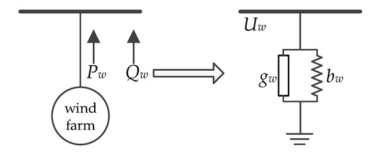
Figure 1.
Equivalent admittance of wind power external characteristics.
When the wind power external characteristics are converted into equivalent grounding admittance, the self-admittance in the system admittance matrix needs to be modified, that is, the self-admittance changes from Yww to Yww’ =Yww + gw + jbw. Since the equivalent grounding admittance does not have the characteristics of a power source, the injection current of the wind power integrated point is regarded as zero, and the node voltage equation is
where subscript g represents the generator node and subscript n represents the common power exchange node. Since only the generator node has an injection current, the node voltage equation can be shrunk to Ig = YsUg, where the expression of Ys is
If two nodes in matrix Ys are selected to shrink, the shrunk result can reflect the electrical connection of these two nodes. The nodes to be shrunk are a and b, and the rest node set is r, then
According to the expression analysis, if the mutual admittance between two nodes in matrix Ys is large, the mutual admittance between these two nodes after being shrunk is also large, indicating that the electrical connection is close. For self-admittance, such as Ysaa and Ysbb, there is no effect on the mutual admittance of nodes after being shrunk, but for self-admittance in Ysrr, as its mode value increases, the mutual admittance in matrix Ys’ will be reduced. It is worth noting that once the grid structure is completed, the admittance matrix Y is basically unchanged. Hence, when considering the wind power integrated to the system, the admittance matrix Y will change, so as to change the electrical connection between nodes in the system. Therefore, the utilization of wind power to adjust the electrical connection has a theoretical basis.
3.2. The Splitting Optimal Strategy and Bi-Level Planning Model
In order to more intuitively describe the impact of wind power integration on the splitting optimization, Figure 2 shows the schematic diagram in the ideal case. The black node represents the inherent bus node of the system, the green node represents the wind power integrated node, the distance between nodes represents the electrical distance, and different shapes represent different clusters. Before the integration of wind power, the system nodes in the coherence group are scattered, the electrical distance between the groups is short, and the clustering of some nodes is ambiguous. According to the optimization strategy, the appropriate capacity of wind power is integrated into the appropriate location, then the nodes in the coherence group are more closely connected, and the connection degree among different areas is reduced. Therefore, when a large fault causes the system to split, the splitting section will be more likely to locate on the contact line of the coherence group, so as to avoid the internal oscillation of the coherence group.
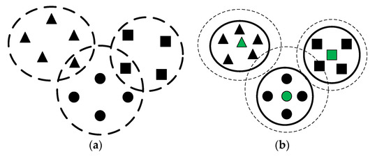
Figure 2.
Optimizing strategy of system splitting considering the integrated wind power. (a) Before optimization; (b) After optimization.
In order to obtain a suitable control scheme to achieve effective clustering, this paper uses a bi-level planning model to find the location-allocation of wind power. The specific process is shown in Figure 3.
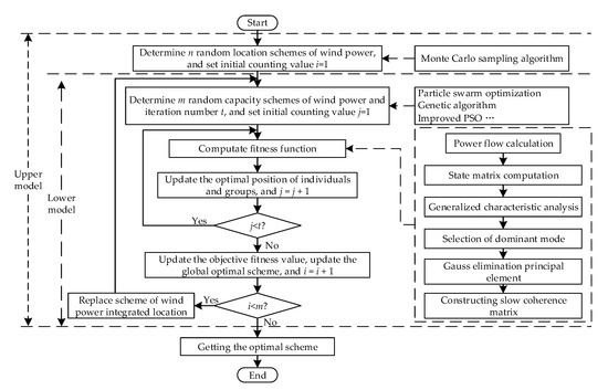
Figure 3.
Flow chart of optimization scheme considering wind power.
The upper model is to select some system nodes as the integrated locations of wind power. Because there is no direct relationship between the selection of system nodes, the upper model can use the Monte Carlo sampling algorithm to randomly select considerable feasible schemes, and finally obtain the optimal integrated location. Assume that Bset represents the set of all buses that are capable of integrated wind power. The array W is [w1 w2 … wm], in which m represents the number of integrated locations, and each element represents the location label, then
For the actual power grid, the integrated location of wind power should be located near the geographical bus with rich wind resources as much as possible to ensure the efficient use of wind energy, so the upper output is fixed, and only the integrated capacity scale needs to be adjusted.
The lower model is to solve the integrated capacity of wind power. When the wind power resources are absorbed to the greatest extent, the active power output of the balance generator should be avoided to be negative. Assume that Pbalance is the active power of the balance generator. The array Z is [z1 z2 … zm], each element in the array represents the integrated capacity of each location, then
It is worth noting that the problem of solving the integrated capacity is a nonlinear complex problem, which is difficult to be solved by the traditional nonlinear programming method, so this paper proposes an improved particle swarm optimization (PSO) intelligent algorithm. The main difference between the improved PSO and the traditional PSO is that the crossover and mutation operations in genetic algorithm (GA) are supplemented. In this improved PSO, the velocity parameters and boundaries of particles can be appropriately increased, hence the global searching ability can be effectively exerted. The convergence of a high-quality solution can be improved by crossover operation for particles with good fitness. As for the particles with poor fitness, they have little significance in the later stage of search, so they can perform a mutation operation, and use the mutation characteristics of GA to mine potential high-quality solutions.
In addition, after wind power is integrated to the system, it needs to meet the constraints in power flow calculation while pursuing high fitness value:
where Sgen is the power of all generators; Sload and Sloss are the load power and loss power, respectively. Meanwhile, the active power PL and reactive power QL of the line needs to meet the upper and lower limit constraints, and the same constraints are applied to the generator active power PG, generator reactive power QG, and the bus voltage Ui.
3.3. Verification Method and Indicators
In order to verify the effectiveness of the proposed scheme for coherence optimization, simulation verification can be carried out by the following three steps:
- (1)
- The upper model uses the sampling algorithm to find the appropriate location of wind power, and the lower model uses the optimization algorithm to obtain the power capacity of each integrated location. The optimization scheme is obtained by iterative calculation.
- (2)
- According to the optimization scheme, the power system simulator for engineering power system simulation software (PSS/E) is used to build a new grid structure and simulate N-1 fault disturbance, and obtain the voltage amplitude and phase angle of all nodes.
- (3)
- K-means clustering analysis is carried out on the node voltage to find out the possible splitting lines and construct the splitting sections, and observe whether the range of splitting section is reduced.
In order to quantify the range change of the splitting section, the lines with higher probability of splitting than the average value are defined as high-probability splitting lines under all test faults. After a lot of fault simulation, the numbers of all lines, splitting lines, and high-probability splitting lines are defined as L, Ls, and Lh, respectively, then it is defined as
where α represents the splitting section and β represents the splitting section with high probability; the smaller these two values, the more centralized the splitting range. At the same time, in case of all faults, the occurrence times of splitting line i and splitting line j with high probability are recorded as Csi and Chj, respectively, then the definition is as follows:
The larger the γ is, the more likely the splitting section will fall on the splitting lines with high probability.
4. Case Study
In order to verify the effectiveness of the proposed scheme, the IEEE 39-bus system was used for analysis. It represents a 345 kV equivalent power network in New England of the United States. The system topology is shown in Figure 4. In the simulation process, the wind turbine in the wind farm adopts the constant power factor model, and its power factor is 0.95. Meanwhile, it assumes that the wind speed remains unchanged during the fault and recovery process, and the main research is to study the influence of wind power location-allocation on the power system coherence when the grid fault occurs.
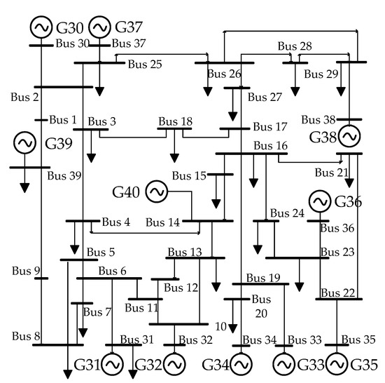
Figure 4.
Topology of IEEE 39-bus system.
4.1. The Influence of Location-allocation of Wind Power
In order to illustrate the influence of wind power on the generator shrinkage admittance matrix, node 10 and node 18 are taken as the integrated locations with 300 MW wind power, and the shrinkage admittance difference is shown in Figure 5.
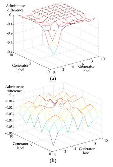
Figure 5.
The influence of wind power on the system shrinkage admittance matrix. (a) Wind power to bus 10; (b) Wind power to bus 18.
In Figure 5, the horizontal axis represents the generator label, and the vertical axis represents the difference between the shrinkage admittance matrix after and before the integration of wind power. Compared with the above figures, it is found that there is a more obvious hollow in Figure 5a, while in Figure 5b, the hollow is even. It mainly lies in that bus 10 is directly connected with bus 32, corresponding to generator 32, thus the integrated wind power has a greater impact on the admittance value of the generator node after shrinkage. However, bus 18 is far away from all generators, so there is no very prominent hollow. Correspondingly, when the integrated capacity of wind power changes, the hollow degree also changes accordingly. According to this analysis, it is effective to consider the influence of the location-allocation of wind power on the electrical connection of the system.
Furthermore, take node 1 as the integrated location, and take 0.6 MW as the step, then get the curves of different integrated capacity and fitness values. The change of node correlation model values under different integrated capacity are shown in Figure 6.
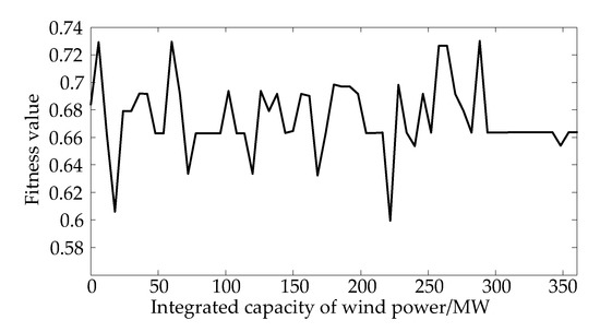
Figure 6.
The influence of integrated capacity of wind power on system fitness value.
It can be seen from Figure 6 that when the integrated capacity of wind power is gradually increased in the same location, the model fitness value does not show a correlation change, which is mainly because, after the integration of wind power, what changes is the overall power flow of the system. When the coherency of a certain area is enhanced due to the change of power flow, it may weaken the coherency of other original coherency areas at the same time. It further shows that this problem is a nonlinear complex problem, so it is reasonable to adopt the improved intelligent optimization algorithm to solve it.
4.2. Slow Coherence Clustering and Fault Simulation
In order to elaborate the calculation process of the slow coherence theory, the IEEE 39-bus system was taken as an example to analyze. There are 10 generators in the grid, corresponding to 10 kinds of electromechanical oscillation modes. After the characteristic calculation, the calculation results of eigenvalues were arranged from small to large, as shown in Table 1.

Table 1.
Generalized eigenvalues of the IEEE 39-bus system.
According to the maximum difference method, there is r = 6, then the system can be divided into 6 groups (including zero mode). According to the eigenvalues, the corresponding eigenvectors are selected to construct the modal matrix, and then the slow coherence correlation matrix S can be calculated by Gaussian elimination. The clustering results are shown in Table 2.
Table 2.
Clustering result of the IEEE 39-bus system.
After the above steps, the slow coherence correlation matrix and node distribution information can be obtained, and the fitness value can be calculated according to the node correlation model. According to this calculation process, assuming that at most 10 nodes can integrate wind power, and the capacity of each node is not limited (but the total capacity should be less than the active output of the balance generator in the initial grid), the bi-level planning model is solved to obtain the appropriate location-allocation scheme of wind power. The upper model uses Monte Carlo sampling algorithm and the sample capacity is 1000. In the lower model, PSO, GA, and improved PSO are used to determine the integrated capacity of each location. The population number is 200 and the number of iterations is 400.
Figure 7 shows the comparison of fitness curves before and after capacity optimization under different integrated location schemes. Each point on the x-axis represents a location scheme, the y-axis represents the fitness value, the blue curve is the fitness result with optimized capacity, and the black curve is the fitness result with random capacity. It can be seen that different location schemes have different coherence effects, but after capacity optimization, the coherence effects can be improved. Therefore, in the actual process, even if the integrated locations of wind power have been determined according to the actual geographical location, only the wind power capacity of each integrated location needs to be adjusted, which can also achieve a better optimization effect to ensure the splitting section appearing in the no-coherence area as much as possible.
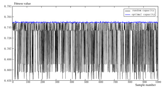
Figure 7.
Optimization effect distribution under different location schemes.
In order to verify the superiority of the improved PSO algorithm, take the same sample number and iteration times for each optimization algorithm. The calculation results and iterative convergence curve are shown in Table 3 and Figure 8.
Table 3.
Comparison of calculation results under different optimization algorithms.
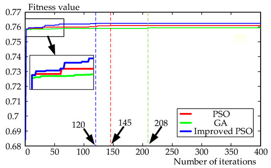
Figure 8.
Comparison of convergence effect.
Comparing the data in Table 3, it reveals that the three algorithms can effectively improve the value of the objective function in the initial grid structure. Meanwhile, in Figure 8, the x-axis represents the number of iterations, the y-axis represents the optimal fitness value. It can be seen that although the difference between the final optimization results of the improved algorithm and the traditional algorithms is not obvious, the improved algorithm needs less iterations to converge. As shown in Figure 8, the improved PSO algorithm needs 120 iterations to achieve convergence; nevertheless, the iterations of PSO and GA are 145 and 208, respectively. Therefore, the improved PSO algorithm has a better effect on solving this problem.
Table 4 gives the suggestions for the location-allocation scheme of wind power under the proposed optimization strategy. In order to verify the effectiveness of the scheme, PSS/E is used to simulate N-1 faults and analyze the coherency of nodes in the coherency group before and after the integration of wind power.
Table 4.
Distribution of the location-allocation of wind power in the IEEE 39-bus system.
Figure 9 shows the comparison diagram of node phase angle curves under three kinds of N-1 faults: (1) three-phase short-circuit fault occurs in line 7–8 at 1.0 s, and the fault is removed at 1.5 s; (2) three-phase short-circuit fault occurs in line 10–11 at 1.0 s, and the fault is removed at 1.7 s; (3) three-phase short-circuit fault occurs in line 25–37 at 1.0 s, and the fault is removed at 1.7 s. In Figure 9, the x-axis represents the fault simulation time and the y-axis represents the voltage phase angle of the system node. It can be found that, after optimization, the number of clustering groups is less, and the oscillation deviation of nodes belonging to the same clustering group is reduced, which indicates that the coherency is enhanced.
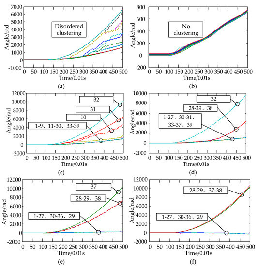
Figure 9.
Comparison diagram of node phase angle before and after optimization of the IEEE 39-bus system under different faults. (a) Before optimization of fault 1; (b) After optimization of fault 1; (c) Before optimization of fault 2 (d) After optimization of fault 2; (e) Before optimization of fault 3; (f) After optimization of fault 3.
Further, all the N-1 faults are simulated to find all the splitting lines and calculate the decision space of high-probability splitting. The calculation results are listed as Table 5.
Table 5.
Comparison of splitting range before and after optimization under N-1 faults.
According to the data comparison in Table 5, the reduction of the splitting section and the decision space of the splitting section with high probability, as well the increase of average splitting frequency of splitting lines with high probability, indicate that the splitting section will fall in a certain range more likely when a fault occurs. Figure 10 clearly compares the change of splitting range. The gray area represents the decision space of splitting with high probability. It can be seen that adding certain capacity of wind power in specified locations can effectively concentrate the splitting range in a small area, which is convenient for splitting control.
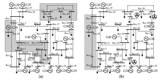
Figure 10.
Comparison of splitting decision space before and after optimization. (a) Splitting decision space before optimization; (b) Splitting decision space after optimization.
5. Conclusions
In this paper, by studying the influence of wind power on electrical connection, a bi-level planning method for splitting control with improved intelligent algorithm was proposed. This method can centralize the splitting section and reduce the difficulty of splitting control by adjusting the location-allocation of wind power. The following conclusions can be drawn:
- Based on the slow coherence theory, it was found that the electrical connections among nodes are related to the system admittance matrix. For the system with determined grid structure, the location-allocation of wind power can be considered to realize the strong coupling within the coherence group.
- According to the simulation of the IEEE 39-bus system, the indicator representing the splitting range has changed from 86.96% to 60.87%, and the proportion of lines with high-probability splitting decreased from 30.43% to 13.04%, which represents the reduction of splitting range and verifies the effectiveness of the method.
- It is worth noting that this method can concentrate the large probability of the splitting section in a certain range under lots of faults. It does not mean that the splitting only appears in this range, but it can reduce the probability of splitting in other ranges.
- In future research, the impact of wind turbine transient characteristics on the splitting optimization and the cost constraints can be considered to ensure more application in practical engineering.
Author Contributions
The authors confirm their contributions to the paper as follows: F.T. and W.L. proposed the idea and wrote the paper; C.W. and X.G. revised the manuscript; B.H. and F.Q. reviewed the results and approved the final version of the manuscript. All authors have read and agreed to the published version of the manuscript.
Funding
This study was funded by the National Natural Science Foundation of China (grant number 51977157).
Acknowledgments
We sincerely thank the editor and the anonymous reviewers of the paper for their kind support. We also want to thank the Grid Corporation for providing relevant information and data.
Conflicts of Interest
The authors declare no conflict of interest.
Nomenclature
| Parameters | |
| Mi | inertia of generator i |
| Pmi | mechanical power of generator i |
| Pei | electromagnetic power of generator i |
| Di | damping coefficient of generator i |
| K | system state matrix |
| A | state matrix |
| G | the real part of admittance matrix |
| B | the imaginary part of admittance matrix |
| λ | eigenvalue of state matrix |
| v | eigenvector of state matrix |
| E | diagonal square matrix |
| p | time scale value |
| r | number of dominant modes of eigenvalues |
| ĸ | a small positive number |
| k | Column k of matrix S |
| η | calculation result between [0,1] |
| gw | equivalent conductance of wind power external characteristics |
| bw | equivalent susceptance of wind power external characteristics |
| Yww | self-admittance of wind power output point |
| Yww’ | modified self-admittance of wind power output point |
| Ys | admittance matrix shrunk to each synchronous generator point |
| Variables | |
| δi | power angle of generator i |
| ωi | angular velocity of generator i |
| ω0 | reference angular velocity |
| ∆δ | the change of generator power angle relative to balance position |
| the second derivative of ∆δ to time | |
| Ei, Ej | voltage amplitude of nodes i and j |
| δij | voltage phase angle difference between nodes i and j |
| V | modal matrix |
| S | slow coherence correlation matrix |
| H | normalization matrix of matrix S |
| Ha | The a-th coherence matrix in matrix H |
| F | fitness value |
| vmax | average value of coherence degree between a node and its coherence group |
| vrest | average value of coherence degree between a node and other coherence groups |
| average value of column j of matrix Ha | |
| Haij | the element of row i and column j of matrix Ha |
| e | the standard deviation of each column coherence degree in each group matrix |
| sa | rows of matrix Ha |
| Pw | active power of wind farm |
| Qw | reactive power of wind farm |
| Uw | wind power output point voltage |
| Ig | synchronous generator output point current |
| Ug | synchronous generator output point voltage |
| W | the set of w |
| w | bus label of wind power integrated location |
| Bset | the set of all buses that are capable of integrated wind power |
| Z | the set of z |
| z | the wind power integrated capacity of each integrated location |
| Pbalance | the original active power of the balance generator |
| Sgen | generator output power |
| Sload | load power |
| Sloss | loss power |
| PL | line active power |
| QL | line reactive power |
| PG | generator active power |
| QG | generator reactive power |
| Ui | voltage of bus i |
| L | the number of all lines |
| Ls | splitting lines |
| Lh | high-probability splitting lines |
| α | the splitting section |
| β | the splitting section with high probability |
| Csi | the occurrence times of the splitting line i in case of all faults |
| Chj | the high probability splitting line j in case of all faults |
| γ | average splitting frequency of high probability splitting lines |
References
- Licia, P.; Carlos, R.M. The Venezuelan energy crisis: Renewable energies in the transition towards sustainability. Renew. Sustain. Energy Rev. 2019, 105, 415–426. [Google Scholar]
- Luo, J.B.; Chen, Y.H.; Liu, Q. Overview of large-scale intermittent new energy grid-connected control technology. Power Syst. Prot. Control 2014, 42, 140–146. [Google Scholar]
- Liu, Y.; Qin, W.P.; Han, X.Q. Modelling of large-scale wind/solar hybrid system and influence analysis on power system transient voltage stability. In Proceedings of the 2017 12th IEEE Conference on Industrial Electronics and Applications (ICIEA), Siem Reap, Cambodia, 18–20 June 2017; pp. 477–482. [Google Scholar]
- Chowdhury, M.; Shen, W. Transient stability of power system integrated with doubly fed induction generator wind farms. IET Renew. Power Gener. 2015, 9, 184–194. [Google Scholar] [CrossRef]
- Tang, W.Q.Y.; Hu, J.B.; Chang, Y.Z. Modeling of DFIG-Based Wind Turbine for Power System Transient Response Analysis in Rotor Speed Control Timescale. IEEE Trans. Power Syst. 2018, 33, 6795–6805. [Google Scholar] [CrossRef]
- De Almeida, R.G.; Lopes, J.A.P. Participation of doubly fed induction wind generators in system frequency regulation. IEEE Trans. Power Syst. 2007, 22, 944–950. [Google Scholar] [CrossRef]
- Li, Y.; Fan, L.L.; Miao, Z.X. Wind in Weak Grids: Low-Frequency Oscillations, Subsynchronous Oscillations, and Torsional Interactions. IEEE Trans. Power Syst. 2020, 35, 109–118. [Google Scholar] [CrossRef]
- Lei, Y.Z.; Mullane, A.; Lightbody, G. Modeling of the wind turbine with a doubly fed induction generator for grid integration studies. IEEE Trans. Energy Convers. 2006, 21, 257–264. [Google Scholar] [CrossRef]
- Fan, Q.; Wen, X.K.; Xu, M.M. Research and Simulation Analysis on Transient Stability of Wind Power Accessing in Regional Grid. In Proceedings of the 2018 2nd IEEE Advanced Information Management, Communicates, Electronic and Automation Control Conference (IMCEC), Xi’an, China, 25–27 May 2018; pp. 389–393. [Google Scholar]
- Zhang, M.; Li, Q.; Liu, C. An Aggregation Modeling Method of Large-scale Wind Farms in Power System Transient Stability Analysis. In Proceedings of the 2018 International Conference on Power System Technology (POWERCON), Guangzhou, China, 6–8 November 2018; pp. 1351–1356. [Google Scholar]
- Liu, J.L.; Tang, F.; Liao, Q.F. Influence of DFIG access on out of step oscillation center migration of power system. Grid Technol. 2017, 41, 2561–2568. [Google Scholar]
- Liu, M.Y.; Pan, W.X.; Zhang, Y.B. A Dynamic Equivalent Model for DFIG-Based Wind Farms. IEEE Access 2019, 7, 74931–74940. [Google Scholar] [CrossRef]
- Liu, Q.; Gao, J.T.; Ding, J. The influence research of large-scale wind power on out-of-step oscillation of the Northwest China Power Grid. In Proceedings of the 2015 5th International Conference on Electric Utility Deregulation and Restructuring and Power Technologies (DRPT), Changsha, China, 26–29 November 2015; pp. 1080–1084. [Google Scholar]
- Haddadi, A.; Kocar, I.; Karaagac, U. Impact of Wind Generation on Power Swing Protection. IEEE Trans. Power Deliv. 2019, 34, 1118–1128. [Google Scholar] [CrossRef]
- Neumann, T.; Feltes, C.; Erlich, I. Response of DFG-based wind farms operating on weak grids to voltage sags. In Proceedings of the 2011 IEEE Power and Energy Society General Meeting, Detroit, MI, USA, 24–28 July 2011; pp. 1–6. [Google Scholar]
- Yousefian, R.; Bhattarai, R. Transient stability enhancement of power grid with integrated wide area control of wind farms and synchronous generators. IEEE Trans. Power Syst. 2016, 32, 4818–4831. [Google Scholar] [CrossRef]
- Tang, F.; Liu, Y.; Shi, H.B. A fast active decoupling strategy for large power grids considering wind farm interconnection. J. Elect. Technol. 2019, 34, 2092–2101. [Google Scholar]
- Liu, Y.; Tang, F.; Shi, H.B. An online homology identification strategy for power system considering wind farm connection. Power Syst. Technol. 2019, 43, 1236–1245. [Google Scholar]
- Qiao, Y.; Shen, C.; Lu, Q. Islanding decision space minimization and quick search in case of large-scale grids. Proc. CSEE 2008, 28, 23–28. [Google Scholar]
- Ni, J.M.; Shen, C.; Chen, Q. Adaptive Islanding Control Based on Slow Coherency (part two): Practical Area Partition Method. Proc. CSEE 2014, 34, 4865–4875. [Google Scholar]
- Song, H.L.; Wu, J.Y.; Ji, L.Y. Generator online coherence recognition based on slow coherence theory and Hilbert-Huang transform. Electr. Power Autom. Equip. 2013, 33, 70–76. [Google Scholar]
- Avramovic, B.; Kokotovic, P.V.; Winkelman, J.R. Area Decomposition for Electromechanical Models of Power Systems. Automatica 1980, 16, 637–648. [Google Scholar] [CrossRef]
- Chow, J.H.; Galarza, R.; Accari, P. Inertial and slow coherency aggregation algorithms for power system dynamic model reduction. IEEE Trans. Power Syst. 1995, 10, 680–685. [Google Scholar] [CrossRef]
- Liu, M.B. Slow coherence partitioning algorithm for dynamic equivalence of multi-machine power systems. J. South China Univ. Technol. (Nat. Sci. Ed.) 1996, 24, 122–130. [Google Scholar]
- Gautam, D.; Vittal, V.; Harbour, T. Impact of Increased Penetration of DFIG-Based Wind Turbine Generators on Transient and Small Signal Stability of Power Systems. IEEE Trans. Power Syst. 2009, 24, 1426–1434. [Google Scholar] [CrossRef]
© 2020 by the authors. Licensee MDPI, Basel, Switzerland. This article is an open access article distributed under the terms and conditions of the Creative Commons Attribution (CC BY) license (http://creativecommons.org/licenses/by/4.0/).