Feasibility of Stochastic Models for Evaluation of Potential Factors for Safety: A Case Study in Southern Italy

 ,
,  ,
,  ,
,  ,
,  and
and 
Abstract
1. Introduction
2. Methodology
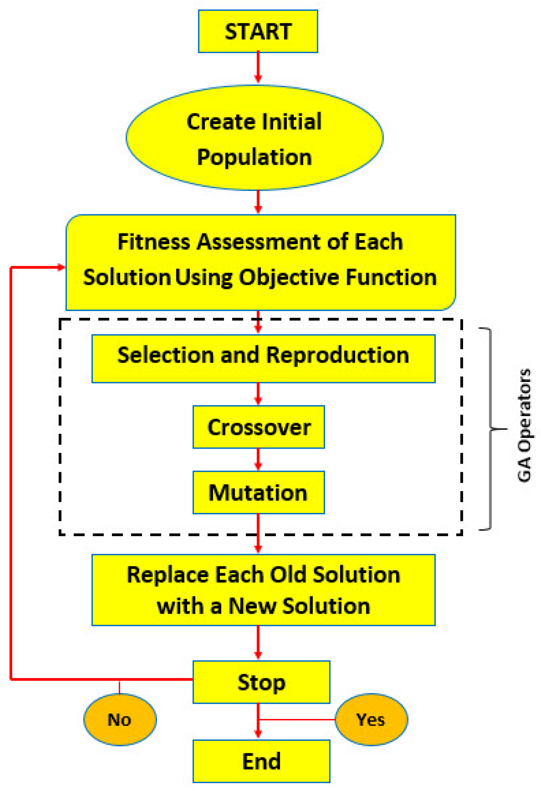
2.1. Genetic Algorithm (GA)
2.2. Particle Swarm Optimization (PSO)
2.3. The Optimization Function and the Correlation Analysis Method
3. Data Collection and Preparation
3.1. Crash, Traffic, and Speed Data
3.2. Correlation Data Analysis
4. Particle Swarm Optimization Modeling for Urban and Rural Area
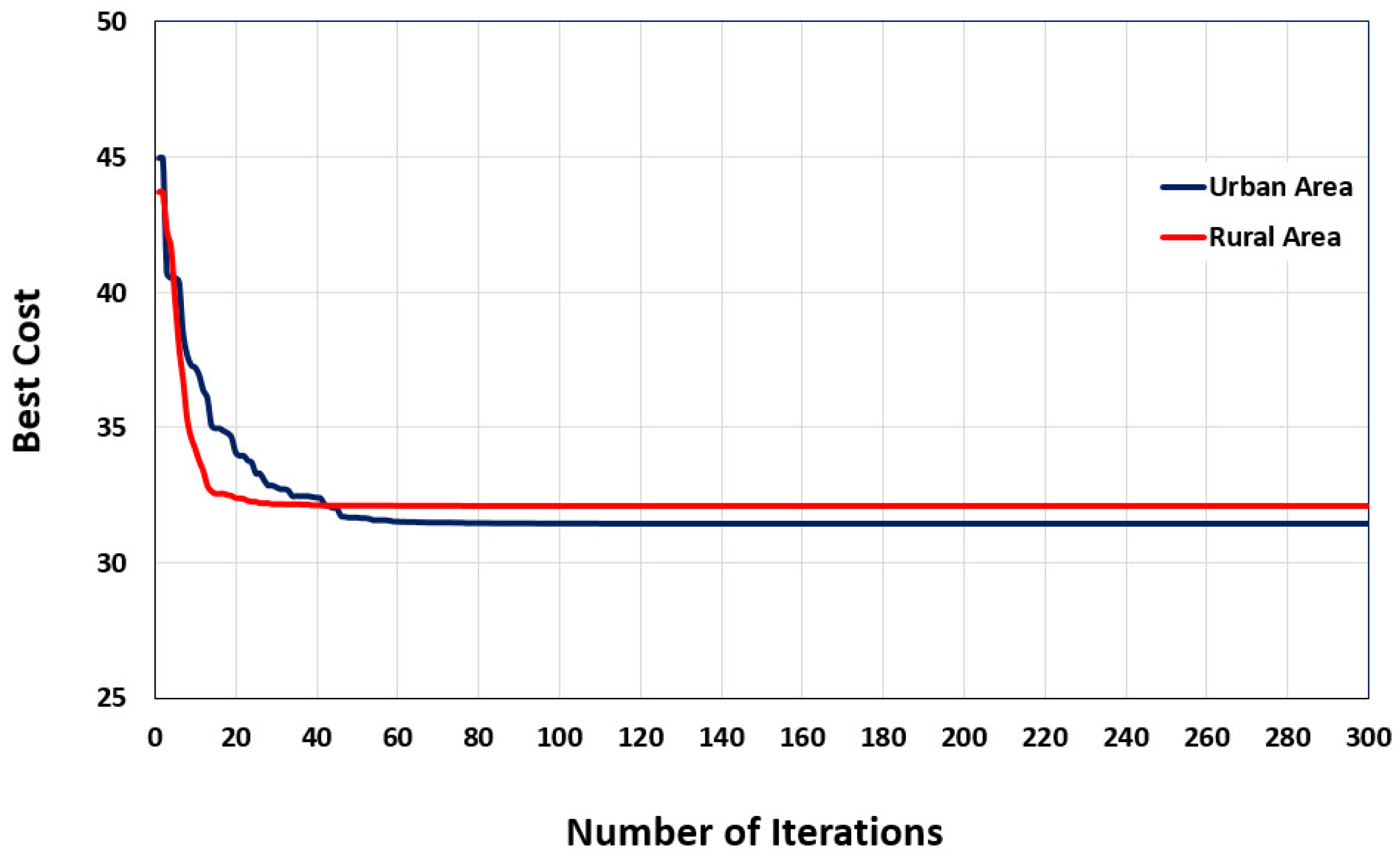
5. Genetic Algorithm Modeling for Urban and Rural Areas
6. Results and Discussion
7. Conclusions
Author Contributions
Funding
Conflicts of Interest
References
- Blas, E.; Kurup, A.S. (Eds.) Equity, Social Determinants and Public Health Programmes; World Health Organization: Geneva, Switzerland, 2010. [Google Scholar]
- Li, Y.; Ma, D.; Zhu, M.; Zeng, Z.; Wang, Y. Identification of significant factors in fatal-injury highway crashes using genetic algorithm and neural network. Accid. Anal. Prev. 2018, 111, 354–363. [Google Scholar] [CrossRef] [PubMed]
- Jovanis, P.P.; Chang, H.L. Modeling the relationship of accidents to miles traveled. Transp. Res. Board 1986, 1068, 42–51. [Google Scholar]
- Poch, M.; Mannering, F. Negative binomial analysis of intersection-accident frequencies. J. Transp. Eng. 1996, 122, 105–113. [Google Scholar] [CrossRef]
- Shankar, V.; Milton, J.; Mannering, F. Modeling accident frequencies as zero-altered probability processes: An empirical inquiry. Accid. Anal. Prev. 1997, 29, 829–837. [Google Scholar] [CrossRef]
- Milton, J.; Mannering, F. The relationship among highway geometrics, traffic-related elements and motor-vehicle accident frequencies. Transportation 1998, 25, 395–413. [Google Scholar] [CrossRef]
- Hadi, M.A.; Aruldhas, J.; Chow, L.; Wattleworth, J.A. Estimating safety effects of cross-section design for various highway types using negative binomial regression. Transp. Res. Rec. 1995, 1500, 169–177. [Google Scholar]
- Miaou, S.P. The relationship between truck accidents and geometric design of road sections: Poisson versus negative binomial regressions. Accid. Anal. Prev. 1994, 26, 471–481. [Google Scholar] [CrossRef]
- Lee, J.; Mannering, F. Impact of roadside features on the frequency and severity of run-off-roadway accidents: An empirical analysis. Accid. Anal. Prev. 2020, 34, 149–161. [Google Scholar] [CrossRef]
- Lord, D.; Mannering, F. The statistical analysis of crash-frequency data: A review and assessment of methodological alternatives. Transp. Res. Part A Policy Pract. 2010, 44, 291–305. [Google Scholar] [CrossRef]
- Mannering, F.L.; Shankar, V.; Bhat, C.R. Unobserved heterogeneity and the statistical analysis of highway accident data. Anal. Methods Accid. Res. 2016, 11, 1–16. [Google Scholar] [CrossRef]
- Mannering, F. Temporal instability and the analysis of highway accident data. Anal. Methods Accid. Res. 2018, 17, 1–13. [Google Scholar] [CrossRef]
- Park, E.S.; Lord, D. Multivariate Poisson-lognormal models for jointly modeling crash frequency by severity. Transp. Res. Rec. 2007, 2019, 1–6. [Google Scholar] [CrossRef]
- El-Basyouny, K.; Sayed, T. Accident prediction models with random corridor parameters. Accid. Anal. Prev. 2009, 41, 1118–1123. [Google Scholar] [CrossRef] [PubMed]
- Anastasopoulos, P.C.; Mannering, F.L. A note on modeling vehicle accident frequencies with random-parameters count models. Accid. Anal. Prev. 2009, 41, 153–159. [Google Scholar] [CrossRef] [PubMed]
- Abduljabbar, R.; Dia, H.; Liyanage, S.; Bagloee, S.A. Applications of artificial intelligence in transport: An overview. Sustainability 2019, 11, 189. [Google Scholar] [CrossRef]
- Karlaftis, M.G.; Golias, I. Effects of road geometry and traffic volumes on rural roadway accident rates. Accid. Anal. Prev. 2002, 34, 357–365. [Google Scholar] [CrossRef]
- Abdel-Aty, M.; Keller, J. Exploring the overall and specific crash severity levels at signalized intersections. Accid. Anal. Prev. 2005, 37, 417–425. [Google Scholar] [CrossRef]
- Park, Y.J.; Saccomanno, F.F. Collision frequency analysis using tree-based stratification. Transp. Res. Rec. 2005, 1908, 121–129. [Google Scholar] [CrossRef]
- Yuan, F.; Cheu, R.L. Incident detection using support vector machines. Transp. Res. Part C Emerg. Technol. 2003, 11, 309–328. [Google Scholar] [CrossRef]
- Yao, B.; Hu, P.; Zhang, M.; Jin, M. A support vector machine with the tabu search algorithm for freeway incident detection. Int. J. Appl. Math. Comput. Sci. 2014, 24, 397–404. [Google Scholar] [CrossRef]
- Siddiqui, C.; Abdel-Aty, M.; Huang, H. Aggregate nonparametric safety analysis of traffic zones. Accid. Anal. Prev. 2012, 45, 317–325. [Google Scholar] [CrossRef] [PubMed]
- Li, Z.; Liu, P.; Wang, W.; Xu, C. Using support vector machine models for crash injury severity analysis. Accid. Anal. Prev. 2012, 45, 478–486. [Google Scholar] [CrossRef]
- Chen, C.; Zhang, G.; Qian, Z.; Tarefder, R.A.; Tian, Z. Investigating driver injury severity patterns in rollover crashes using support vector machine models. Accid. Anal. Prev. 2016, 90, 128–139. [Google Scholar] [CrossRef] [PubMed]
- Holland, J.H. Adaptation in Natural and Artificial Systems; University of Michigan Press: Ann Arbor, MI, USA, 1975. [Google Scholar]
- Arbis, D.; Dixit, V.V. Game theoretic model for lane changing: Incorporating conflict risks. Accid. Anal. Prev. 2019, 125, 158–164. [Google Scholar] [CrossRef] [PubMed]
- Kim, Y.H.; Yoon, Y.; Geem, Z.W. A comparison study of harmony search and genetic algorithm for the max-cut problem. Swarm Evol. Comput. 2019, 44, 130–135. [Google Scholar] [CrossRef]
- Aryafar, A.; Mikaeil, R.; Shafiee Haghshenas, S.; Shafiei Haghshenas, S. Utilization of soft computing for evaluating the performance of stone sawing machines, Iranian Quarries. Int. J. Min. Geo-Eng. 2018, 52, 31–36. [Google Scholar]
- Fakharian, P.; Naderpour, H.; Haddad, A.; Rafiean, A.H.; Eidgahee, D.R. A proposed model for compressive strength prediction of FRP-confined rectangular column in terms of Genetic expression Programming (GEP). Concr. Res. 2018, 11, 5–18. [Google Scholar]
- Haghshenas, S.S.; Faradonbeh, R.S.; Mikaeil, R.; Haghshenas, S.S.; Taheri, A.; Saghatforoush, A.; Dormishi, A. A new conventional criterion for the performance evaluation of gang saw machines. Measurement 2019, 146, 159–170. [Google Scholar] [CrossRef]
- Pinto, B.Q.; Ribeiro, C.C.; Rosseti, I.; Noronha, T.F. A biased random-key genetic algorithm for routing and wavelength assignment under a sliding scheduled traffic model. J. Glob. Optim. 2020, 77, 949–973. [Google Scholar] [CrossRef]
- Luan, J.; Yao, Z.; Zhao, F.; Song, X. A novel method to solve supplier selection problem: Hybrid algorithm of genetic algorithm and ant colony optimization. Math. Comput. Simul. 2019, 156, 294–309. [Google Scholar] [CrossRef]
- Hosseini, S.M.; Ataei, M.; Khalokakaei, R.; Mikaeil, R.; Haghshenas, S.S. Study of the effect of the cooling and lubricant fluid on the cutting performance of dimension stone through artificial intelligence models. Eng. Sci. Technol. Int. J. 2020, 23, 71–81. [Google Scholar] [CrossRef]
- Salemi, A.; Mikaeil, R.; Haghshenas, S.S. Integration of Finite Difference Method and Genetic Algorithm to Seismic analysis of Circular Shallow Tunnels (Case Study: Tabriz Urban Railway Tunnels). KSCE J. Civ. Eng. 2017, 22, 1978–1990. [Google Scholar] [CrossRef]
- Slowik, A.; Kwasnicka, H. Nature inspired methods and their industry applications—Swarm intelligence algorithms. IEEE Trans. Ind. Inform. 2018, 14, 1004–1015. [Google Scholar] [CrossRef]
- Dulebenets, M.A. A Comprehensive Evaluation of Weak and Strong Mutation Mechanisms in Evolutionary Algorithms for Truck Scheduling at Cross-Docking Terminals. IEEE Access 2018, 6, 65635–65650. [Google Scholar] [CrossRef]
- Brezočnik, L.; Fister, I.; Podgorelec, V. Swarm intelligence algorithms for feature selection: A review. Appl. Sci. 2018, 8, 1521. [Google Scholar] [CrossRef]
- Anandakumar, H.; Umamaheswari, K. A bio-inspired swarm intelligence technique for social aware cognitive radio handovers. Comput. Electr. Eng. 2018, 71, 925–937. [Google Scholar] [CrossRef]
- Zhao, X.; Wang, C.; Su, J.; Wang, J. Research and application based on the swarm intelligence algorithm and artificial intelligence for wind farm decision system. Renew. Energy 2019, 134, 681–697. [Google Scholar] [CrossRef]
- Dulebenets, M.A. An Adaptive Island Evolutionary Algorithm for the berth scheduling problem. Memetic Comput. 2020, 12, 51–72. [Google Scholar] [CrossRef]
- Kandiri, A.; Golafshani, E.M.; Behnood, A. Estimation of the compressive strength of concretes containing ground granulated blast furnace slag using hybridized multi-objective ANN and salp swarm algorithm. Constr. Build. Mater. 2020, 248, 118676. [Google Scholar] [CrossRef]
- Mikaeil, R.; Haghshenas, S.S.; Haghshenas, S.S.; Ataei, M. Performance prediction of circular saw machine using imperialist competitive algorithm and fuzzy clustering technique. Neural Comput. Appl. 2018, 29, 283–292. [Google Scholar] [CrossRef]
- Mikaeil, R.; Haghshenas, S.S.; Hoseinie, S.H. Rock penetrability classification using artificial bee colony (ABC) algorithm and self-organizing map. Geotech. Geol. Eng. 2018, 36, 1309–1318. [Google Scholar] [CrossRef]
- Mikaeil, R.; Haghshenas, S.S.; Ozcelik, Y.; Gharehgheshlagh, H.H. Performance evaluation of adaptive neuro-fuzzy inference system and group method of data handling-type neural network for estimating wear rate of diamond wire saw. Geotech. Geol. Eng. 2018, 36, 3779–3791. [Google Scholar] [CrossRef]
- Mikaeil, R.; Haghshenas, S.S.; Sedaghati, Z. Geotechnical risk evaluation of tunneling projects using optimization techniques (case study: The second part of Emamzade Hashem tunnel). Nat. Hazards 2019, 97, 1099–1113. [Google Scholar] [CrossRef]
- Mikaeil, R.; Beigmohammadi, M.; Bakhtavar, E.; Haghshenas, S.S. Assessment of risks of tunneling project in Iran using artificial bee colony algorithm. SN Appl. Sci. 2019, 1, 1711. [Google Scholar] [CrossRef]
- Dormishi, A.; Ataei, M.; Mikaeil, R.; Khalokakaei, R.; Haghshenas, S.S. Evaluation of gang saws’ performance in the carbonate rock cutting process using feasibility of intelligent approaches. Eng. Sci. Technol. Int. J. 2019, 22, 990–1000. [Google Scholar] [CrossRef]
- Faradonbeh, R.S.; Haghshenas, S.S.; Taheri, A.; Mikaeil, R. Application of self-organizing map and fuzzy c-mean techniques for rockburst clustering in deep underground projects. Neural Comput. Appl. 2020, 32, 8545–8559. [Google Scholar]
- Fiorini Morosini, A.; Shaffiee Haghshenas, S.; Shaffiee Haghshenas, S.; Geem, Z.W. Development of a Binary Model for Evaluating Water Distribution Systems by a Pressure Driven Analysis (PDA) Approach. Appl. Sci. 2020, 10, 3029. [Google Scholar] [CrossRef]
- Sarkar, S.; Vinay, S.; Raj, R.; Maiti, J.; Mitra, P. Application of optimized machine learning techniques for prediction of occupational accidents. Comput. Oper. Res. 2019, 106, 210–224. [Google Scholar] [CrossRef]
- Liu, Y.; Zou, B.; Ni, A.; Gao, L.; Zhang, C. Calibrating microscopic traffic simulators using machine learning and particle swarm optimization. Transp. Lett. 2020, 1–13. [Google Scholar] [CrossRef]
- Kennedy, J.; Eberhart, R. Particle swarm optimization. In Proceedings of the ICNN’95-International Conference on Neural Networks, Perth, WA, Australia, 27 November–1 December 1995; pp. 1942–1948. [Google Scholar]
- Poli, R.; Kennedy, J.; Blackwell, T. Particle swarm optimization. Swarm Intell. 2007, 1, 33–57. [Google Scholar] [CrossRef]
- Frank, L.R.; Ferreira, Y.M.; Julio, E.P.; Ferreira, F.H.C.; Dembogurski, B.J.; Silva, E.F. Multilayer Perceptron and Particle Swarm Optimization Applied to Traffic Flow Prediction on Smart Cities. In International Conference on Computational Science and Its Applications; Springer: Cham, Switzerland, 2019; pp. 35–47. [Google Scholar]
- Chen, L.; Monteiro, T.; Wang, T.; Marcon, E. Design of shared unit-dose drug distribution network using multi-level particle swarm optimization. Health Care Manag. Sci. 2019, 22, 304–317. [Google Scholar] [CrossRef] [PubMed]
- Liu, P.; Xie, M.; Bian, J.; Li, H.; Song, L. A Hybrid PSO–SVM Model Based on Safety Risk Prediction for the Design Process in Metro Station Construction. Int. J. Environ. Res. Public Health 2020, 17, 1714. [Google Scholar] [CrossRef] [PubMed]
- Tharwat, A.; Elhoseny, M.; Hassanien, A.E.; Gabel, T.; Kumar, A. Intelligent Bézier curve-based path planning model using Chaotic Particle Swarm Optimization algorithm. Clust. Comput. 2019, 22, 4745–4766. [Google Scholar] [CrossRef]
- Noori, A.M.; Mikaeil, R.; Mokhtarian, M.; Haghshenas, S.S.; Foroughi, M. Feasibility of intelligent models for prediction of utilization factor of TBM. Geotech. Geol. Eng. 2020, 38, 3125–3143. [Google Scholar] [CrossRef]
- Lloyd, S. Least squares quantization in PCM. IEEE Trans. Inf. Theory 1982, 28, 129–137. [Google Scholar] [CrossRef]
- Feng, X.; Li, S.; Yuan, C.; Zeng, P.; Sun, Y. Prediction of slope stability using naive Bayes classifier. KSCE J. Civ. 2018, 22, 941–950. [Google Scholar] [CrossRef]
- Hosseini, S.M.; Ataei, M.; Khalokakaei, R.; Mikaeil, R.; Haghshenas, S.S. Investigating the Role of the Cooling and Lubricant Fluids on the Performance of Cutting Disks (Case Study: Hard Rocks). Rud. Geološko Naft. Zb. 2019, 34. [Google Scholar]
- Pirouz, B.; Shaffiee Haghshenas, S.; Shaffiee Haghshenas, S.; Piro, P. Investigating a serious challenge in the sustainable development process: Analysis of confirmed cases of COVID-19 (new type of coronavirus) through a binary classification using artificial intelligence and regression analysis. Sustainability 2020, 12, 2427. [Google Scholar] [CrossRef]
- Mussone, L.; Bassani, M.; Masci, P. Analysis of factors affecting the severity of crashes in urban road intersections. Accid. Anal. Prev. 2019, 103, 112–122. [Google Scholar] [CrossRef]
- Dutta, N.; Fontaine, M.D. Improving freeway segment crash prediction models by including disaggregate speed data from different sources. Accid. Anal. Prev. 2019, 132, 1–16. [Google Scholar] [CrossRef]
- Dormishi, A.R.; Ataei, M.; Khaloo Kakaie, R.; Mikaeil, R.; Shaffiee Haghshenas, S. Performance evaluation of gang saw using hybrid ANFIS-DE and hybrid ANFIS-PSO algorithms. J. Min. Environ 2020, 10, 543–557. [Google Scholar]
- Shaffiee Haghshenas, S.; Pirouz, B.; Shaffiee Haghshenas, S.; Pirouz, B.; Piro, P.; Na, K.S.; Geem, Z.W. Prioritizing and Analyzing the Role of Climate and Urban Parameters in the Confirmed Cases of COVID-19 Based on Artificial Intelligence Applications. Int. J. Env. Res. Public Health 2020, 17, 3730. [Google Scholar] [CrossRef] [PubMed]
- Mikaeil, R.; Bakhshinezhad, H.; Haghshenas, S.S.; Ataei, M. Stability analysis of tunnel support systems using numerical and intelligent simulations (case study: Kouhin Tunnel of Qazvin-Rasht Railway). Rud. Geološko Naft. Zb. 2019, 34, 1–10. [Google Scholar] [CrossRef]
- Mirjalili, S. Genetic algorithm. In Evolutionary Algorithms and Neural Networks; Springer: Cham, Switzerland, 2019; pp. 43–55. [Google Scholar]


| Data Field Type | Data Field | Description |
|---|---|---|
| Human characteristic | Driver gender | Male or female |
| Vehicle characteristic | Vehicle type | Car, motorcycle, truck, and other |
| Road environment | Road type | National rural road, provincial rural road, national and provincial rural road in urban context, and urban road |
| Other environment | Light conditions | Daylight and nighttime |
| Day of the week | Weekday and weekend | |
| Location environment | Macroarea location | Urban and rural |
| Accident characteristic | Number of vehicles | Number of vehicles involved |
| Accident nature | Way out, collision with an accidental obstacle, side collision, front-side collision, rear-end collision, head-on collision, pedestrian collision, impact with parked vehicle, impact with stopped vehicle, fall from vehicle, and sudden braking | |
| Accident severity | Injuries and deaths |
| Daylight | Weekday | Average Speed | Annual Average Daily Traffic | Number of Vehicles | Type of Accident | |
|---|---|---|---|---|---|---|
| Daylight | 1 | |||||
| Weekday | −0.309 | 1 | ||||
| Average speed | −0.124 | 0.262 | 1 | |||
| Annual average daily traffic | 0.042 | −0.246 | −0.378 | 1 | ||
| Number of vehicles | −0.012 | −0.112 | 0.148 | 0.104 | 1 | |
| Type of accident | −0.035 | −0.029 | 0.06 | 0.028 | 0.182 | 1 |
| Daylight | Weekday | Average Speed | Annual Average Daily Traffic | Number of Vehicles | Type of Accident | |
|---|---|---|---|---|---|---|
| Daylight | 1 | |||||
| Weekday | −0.327 | 1 | ||||
| Average speed | −0.078 | 0.118 | 1 | |||
| Annual average daily traffic | 0.158 | 0.109 | 0.363 | 1 | ||
| Number of vehicles | −0.049 | 0.215 | 0.09 | 0.053 | 1 | |
| Type of accident | −0.204 | 0.279 | −0.08 | 0.023 | 0.396 | 1 |
| Case # | Optimum Partition | Rec. Class | Actual Type of Accident Place | Case # | Optimum Partition | Rec. Class | Actual Type of Accident Place | ||||
|---|---|---|---|---|---|---|---|---|---|---|---|
| The First Class | The Second Class | The Third Class | The First Class | The Second Class | The Third Class | ||||||
| 1 | 0.327 | 1.051 | 1.033 | 1 | Straight | 40 | 0.021 | 1.014 | 1.016 | 1 | Intersection |
| 2 | 0.050 | 1.017 | 1.016 | 1 | Straight | 41 | 0.107 | 1.020 | 1.014 | 1 | Straight |
| 3 | 1.131 | 1.498 | 0.405 | 3 | Other | 42 | 0.471 | 1.096 | 1.114 | 1 | Straight |
| 4 | 1.472 | 0.937 | 1.692 | 2 | Intersection | 43 | 0.227 | 1.054 | 1.063 | 1 | Straight |
| 5 | 1.424 | 0.869 | 1.664 | 2 | Intersection | 44 | 0.997 | 1.321 | 1.398 | 1 | Straight |
| 6 | 0.278 | 1.072 | 1.088 | 1 | Straight | 45 | 0.021 | 1.014 | 1.016 | 1 | Straight |
| 7 | 1.023 | 1.436 | 0.189 | 3 | Other | 46 | 0.389 | 1.101 | 1.125 | 1 | Straight |
| 8 | 0.050 | 1.017 | 1.016 | 1 | Straight | 47 | 0.236 | 1.044 | 1.048 | 1 | Straight |
| 9 | 0.050 | 1.017 | 1.016 | 1 | Straight | 48 | 1.273 | 1.539 | 1.651 | 1 | Straight |
| 10 | 0.358 | 1.065 | 1.043 | 1 | Straight | 49 | 0.255 | 1.043 | 1.026 | 1 | Straight |
| 11 | 0.766 | 1.238 | 1.259 | 1 | Straight | 50 | 0.471 | 1.096 | 1.114 | 1 | Straight |
| 12 | 1.001 | 0.185 | 1.359 | 2 | Intersection | 51 | 1.414 | 0.921 | 1.014 | 2 | Intersection |
| 13 | 0.278 | 1.072 | 1.088 | 1 | Straight | 52 | 1.022 | 0.235 | 1.360 | 2 | Straight |
| 14 | 0.317 | 1.068 | 1.063 | 1 | Straight | 53 | 1.083 | 1.470 | 0.301 | 3 | Straight |
| 15 | 1.485 | 0.952 | 1.727 | 2 | Intersection | 54 | 1.497 | 0.979 | 1.749 | 2 | Intersection |
| 16 | 0.217 | 1.030 | 1.018 | 1 | Straight | 55 | 1.105 | 1.484 | 0.491 | 3 | Other |
| 17 | 1.603 | 1.112 | 1.823 | 2 | Intersection | 56 | 1.010 | 0.193 | 1.355 | 2 | Intersection |
| 18 | 0.205 | 1.047 | 1.052 | 1 | Straight | 57 | 1.586 | 1.792 | 1.224 | 3 | Straight |
| 19 | 1.001 | 0.185 | 1.359 | 2 | Intersection | 58 | 1.023 | 0.234 | 1.359 | 2 | Straight |
| 20 | 0.050 | 1.017 | 1.016 | 1 | Straight | 59 | 1.400 | 1.113 | 1.498 | 2 | Intersection |
| 21 | 0.298 | 1.052 | 1.033 | 1 | Straight | 60 | 0.205 | 1.047 | 1.052 | 1 | Intersection |
| 22 | 0.205 | 1.047 | 1.052 | 1 | Straight | 61 | 0.471 | 1.096 | 1.114 | 1 | Intersection |
| 23 | 1.010 | 1.337 | 1.429 | 1 | Straight | 62 | 1.055 | 1.079 | 0.410 | 3 | Other |
| 24 | 0.217 | 1.029 | 1.022 | 1 | Straight | 63 | 1.481 | 1.132 | 1.075 | 3 | Straight |
| 25 | 0.051 | 1.016 | 1.020 | 1 | Straight | 64 | 0.205 | 1.047 | 1.052 | 1 | Straight |
| 26 | 0.392 | 1.103 | 1.129 | 1 | Straight | 65 | 0.205 | 1.047 | 1.052 | 1 | Straight |
| 27 | 0.021 | 1.014 | 1.016 | 1 | Straight | 66 | 0.019 | 1.014 | 1.014 | 1 | Straight |
| 28 | 0.698 | 1.217 | 1.252 | 1 | Straight | 67 | 0.471 | 1.096 | 1.114 | 1 | Straight |
| 29 | 0.236 | 1.034 | 1.016 | 1 | Straight | 68 | 1.421 | 0.886 | 1.687 | 2 | Intersection |
| 30 | 1.006 | 1.428 | 0.169 | 3 | Other | 69 | 0.189 | 1.039 | 1.052 | 1 | Straight |
| 31 | 0.723 | 1.238 | 1.283 | 1 | Straight | 70 | 1.220 | 0.693 | 1.544 | 2 | Intersection |
| 32 | 0.403 | 1.107 | 1.123 | 1 | Straight | 71 | 0.507 | 1.120 | 1.148 | 1 | Straight |
| 33 | 0.516 | 1.109 | 1.115 | 1 | Straight | 72 | 0.205 | 1.047 | 1.052 | 1 | Straight |
| 34 | 0.471 | 1.096 | 1.114 | 1 | Straight | 73 | 0.255 | 1.043 | 1.026 | 1 | Straight |
| 35 | 0.107 | 1.020 | 1.014 | 1 | Straight | 74 | 0.050 | 1.012 | 1.013 | 1 | Straight |
| 36 | 0.021 | 1.014 | 1.016 | 1 | Straight | 75 | 0.205 | 1.047 | 1.052 | 1 | Straight |
| 37 | 0.166 | 1.000 | 1.359 | 1 | Straight | 76 | 0.050 | 1.012 | 1.013 | 1 | Straight |
| 38 | 1.019 | 1.331 | 1.399 | 1 | Intersection | 77 | 1.023 | 0.226 | 1.358 | 2 | Intersection |
| 39 | 0.471 | 1.096 | 1.114 | 1 | Intersection | ||||||
| Case # | Optimum Partition | Rec. Class | Actual Type of Accident Place | Case # | Optimum Partition | Rec. Class | Actual Type of Accident Place | ||||
|---|---|---|---|---|---|---|---|---|---|---|---|
| The First Class | The Second Class | The Third Class | The First Class | The Second Class | The Third Class | ||||||
| 1 | 0.132 | 1.011 | 1.151 | 1 | Straight | 40 | 1.403 | 0.964 | 1.316 | 2 | Intersection |
| 2 | 1.405 | 1.711 | 0.727 | 3 | Other | 41 | 1.134 | 1.501 | 0.728 | 3 | Other |
| 3 | 0.152 | 1.011 | 1.152 | 1 | Straight | 42 | 0.030 | 1.007 | 1.153 | 1 | Straight |
| 4 | 0.132 | 1.011 | 1.151 | 1 | Straight | 43 | 0.073 | 1.012 | 1.156 | 1 | Straight |
| 5 | 1.422 | 1.725 | 0.775 | 3 | Other | 44 | 0.235 | 1.030 | 1.184 | 1 | Straight |
| 6 | 0.273 | 1.045 | 1.196 | 1 | Straight | 45 | 0.235 | 1.030 | 1.184 | 1 | Straight |
| 7 | 1.436 | 1.029 | 0.781 | 3 | Other | 46 | 0.192 | 1.027 | 1.163 | 1 | Straight |
| 8 | 1.009 | 1.422 | 0.570 | 3 | Other | 47 | 1.740 | 1.405 | 0.899 | 3 | Other |
| 9 | 1.416 | 1.723 | 0.742 | 3 | Other | 48 | 1.011 | 0.183 | 1.241 | 2 | Straight |
| 10 | 0.128 | 1.019 | 1.240 | 1 | Straight | 49 | 0.244 | 1.035 | 1.188 | 1 | Straight |
| 11 | 0.128 | 1.019 | 1.240 | 1 | Straight | 50 | 1.030 | 0.244 | 1.269 | 2 | Straight |
| 12 | 0.116 | 1.000 | 1.239 | 1 | Straight | 51 | 0.126 | 1.014 | 1.154 | 1 | Straight |
| 13 | 1.392 | 0.995 | 1.235 | 2 | Intersection | 52 | 0.273 | 1.045 | 1.196 | 1 | Straight |
| 14 | 0.235 | 1.030 | 1.184 | 1 | Straight | 53 | 1.088 | 1.466 | 0.664 | 3 | Other |
| 15 | 0.235 | 1.030 | 1.184 | 1 | Straight | 54 | 1.036 | 0.215 | 1.249 | 2 | Straight |
| 16 | 1.424 | 1.728 | 0.781 | 3 | Other | 55 | 1.394 | 0.992 | 1.237 | 2 | Intersection |
| 17 | 1.728 | 1.392 | 0.854 | 3 | Other | 56 | 1.389 | 0.984 | 1.236 | 2 | Intersection |
| 18 | 0.235 | 1.030 | 1.184 | 1 | Straight | 57 | 1.436 | 1.029 | 0.781 | 3 | Other |
| 19 | 1.012 | 1.422 | 0.572 | 3 | Other | 58 | 0.235 | 1.030 | 1.184 | 1 | Straight |
| 20 | 0.082 | 1.006 | 1.153 | 1 | Straight | 59 | 0.235 | 1.030 | 1.184 | 1 | Straight |
| 21 | 0.132 | 1.011 | 1.151 | 1 | Straight | 60 | 0.132 | 1.011 | 1.151 | 1 | Straight |
| 22 | 0.152 | 1.011 | 1.152 | 1 | Straight | 61 | 0.235 | 1.030 | 1.184 | 1 | Straight |
| 23 | 1.009 | 1.420 | 0.569 | 3 | Other | 62 | 1.436 | 1.029 | 0.781 | 3 | Other |
| 24 | 0.030 | 1.007 | 1.153 | 1 | Straight | 63 | 1.030 | 0.244 | 1.269 | 2 | Straight |
| 25 | 0.030 | 1.007 | 1.153 | 1 | Straight | 64 | 0.986 | 1.393 | 1.239 | 1 | Intersection |
| 26 | 0.384 | 1.057 | 1.188 | 1 | Other | 65 | 0.030 | 1.007 | 1.153 | 1 | Straight |
| 27 | 1.728 | 1.390 | 0.854 | 3 | Intersection | 66 | 0.321 | 1.046 | 1.175 | 1 | Straight |
| 28 | 0.992 | 1.392 | 1.234 | 1 | Other | 67 | 0.261 | 1.023 | 1.163 | 1 | Straight |
| 29 | 0.235 | 1.030 | 1.184 | 1 | Straight | 68 | 0.177 | 1.024 | 1.160 | 1 | Straight |
| 30 | 0.082 | 1.006 | 1.153 | 1 | Straight | 69 | 1.093 | 1.470 | 0.670 | 3 | Other |
| 31 | 0.428 | 1.073 | 1.200 | 1 | Straight | 70 | 1.425 | 1.024 | 0.742 | 3 | Intersection |
| 32 | 1.030 | 0.244 | 1.269 | 2 | Straight | 71 | 0.030 | 1.007 | 1.153 | 1 | Straight |
| 33 | 1.728 | 1.390 | 0.854 | 3 | Other | 72 | 0.177 | 1.024 | 1.160 | 1 | Straight |
| 34 | 0.235 | 1.030 | 1.184 | 1 | Straight | 73 | 0.315 | 1.060 | 1.208 | 1 | Straight |
| 35 | 0.131 | 1.008 | 1.151 | 1 | Straight | 74 | 1.737 | 1.398 | 0.863 | 3 | Other |
| 36 | 0.244 | 1.035 | 1.188 | 1 | Straight | 75 | 0.382 | 1.067 | 1.191 | 1 | Straight |
| 37 | 1.409 | 0.968 | 1.315 | 2 | Intersection | 76 | 1.398 | 1.009 | 1.240 | 2 | Intersection |
| 38 | 0.235 | 1.030 | 1.184 | 1 | Straight | 77 | 0.177 | 1.024 | 1.160 | 1 | Straight |
| 39 | 1.000 | 1.419 | 0.573 | 3 | Other | ||||||
| Urban Area | ||||||
| Daylight | Weekday | Average Speed (km/h) | Annual Average Daily Traffic (Vehicle/Day) | Number of Vehicles | Type of Accident | |
| Straight | 0.000 | 0.991 | 0.799 | 0.309 | 0.411 | 1.000 |
| Intersection | 1.000 | 0.852 | 0.732 | 0.324 | 0.369 | 1.000 |
| Other | 0.092 | 0.963 | 0.703 | 0.258 | 0.308 | 0.000 |
| Rural Area | ||||||
| Daylight | Weekday | Average Speed (km/h) | Annual Average Daily Traffic (Vehicle /Day) | Number of Vehicles | Type of Accident | |
| Straight | 0.016 | 1.000 | 0.769 | 0.283 | 0.147 | 1.000 |
| Intersection | 0.042 | 1.000 | 0.765 | 0.208 | 0.103 | 0.000 |
| Other | 0.401 | 0.000 | 0.711 | 0.229 | 0.119 | 0.603 |
| Case # | Optimum Partition | Rec. Class | Actual Type of Accident Place | Case # | Optimum Partition | Rec. Class | Actual Type of Accident Place | ||||
|---|---|---|---|---|---|---|---|---|---|---|---|
| The First Class | The Second Class | The Third Class | The First Class | The Second Class | The Third Class | ||||||
| 1 | 0.327 | 1.051 | 1.033 | 1 | Straight | 40 | 0.021 | 1.014 | 1.016 | 1 | Intersection |
| 2 | 0.050 | 1.018 | 1.016 | 1 | Straight | 41 | 0.107 | 1.021 | 1.014 | 1 | Straight |
| 3 | 1.131 | 1.498 | 0.406 | 3 | Other | 42 | 0.471 | 1.096 | 1.113 | 1 | Straight |
| 4 | 1.472 | 0.934 | 1.689 | 2 | Intersection | 43 | 0.227 | 1.054 | 1.063 | 1 | Straight |
| 5 | 1.424 | 0.867 | 1.661 | 2 | Intersection | 44 | 0.996 | 1.320 | 1.397 | 1 | Straight |
| 6 | 0.278 | 1.073 | 1.088 | 1 | Straight | 45 | 0.021 | 1.014 | 1.016 | 1 | Straight |
| 7 | 1.023 | 1.436 | 0.193 | 3 | Other | 46 | 0.389 | 1.101 | 1.124 | 1 | Straight |
| 8 | 0.050 | 1.018 | 1.016 | 1 | Straight | 47 | 0.236 | 1.044 | 1.047 | 1 | Straight |
| 9 | 0.050 | 1.018 | 1.016 | 1 | Straight | 48 | 1.273 | 1.537 | 1.649 | 1 | Straight |
| 10 | 0.358 | 1.066 | 1.043 | 1 | Straight | 49 | 0.255 | 1.044 | 1.027 | 1 | Straight |
| 11 | 0.766 | 1.236 | 1.257 | 1 | Straight | 50 | 0.471 | 1.096 | 1.113 | 1 | Straight |
| 12 | 1.001 | 0.188 | 1.357 | 2 | Intersection | 51 | 1.414 | 1.014 | 0.917 | 3 | Intersection |
| 13 | 0.278 | 1.073 | 1.088 | 1 | Straight | 52 | 1.022 | 0.238 | 1.358 | 2 | Straight |
| 14 | 0.317 | 1.068 | 1.063 | 1 | Straight | 53 | 1.083 | 1.471 | 0.303 | 3 | Straight |
| 15 | 1.484 | 0.949 | 1.723 | 2 | Intersection | 54 | 1.496 | 0.976 | 1.745 | 2 | Intersection |
| 16 | 0.217 | 1.031 | 1.018 | 1 | Straight | 55 | 1.105 | 1.483 | 0.489 | 3 | Other |
| 17 | 1.603 | 1.108 | 1.820 | 2 | Intersection | 56 | 1.010 | 0.196 | 1.352 | 2 | Intersection |
| 18 | 0.205 | 1.048 | 1.052 | 1 | Straight | 57 | 1.585 | 1.790 | 1.222 | 3 | Straight |
| 19 | 1.001 | 0.188 | 1.357 | 2 | Intersection | 58 | 1.023 | 0.237 | 1.356 | 2 | Straight |
| 20 | 0.050 | 1.018 | 1.016 | 1 | Straight | 59 | 1.113 | 1.397 | 1.496 | 1 | Intersection |
| 21 | 0.298 | 1.053 | 1.033 | 1 | Straight | 60 | 0.205 | 1.048 | 1.052 | 1 | Intersection |
| 22 | 0.205 | 1.048 | 1.052 | 1 | Straight | 61 | 0.471 | 1.096 | 1.113 | 1 | Intersection |
| 23 | 1.010 | 1.336 | 1.428 | 1 | Straight | 62 | 0.410 | 1.079 | 1.054 | 1 | Other |
| 24 | 0.217 | 1.030 | 1.022 | 1 | Straight | 63 | 1.481 | 1.132 | 1.072 | 3 | Straight |
| 25 | 0.051 | 1.016 | 1.020 | 1 | Straight | 64 | 0.205 | 1.048 | 1.052 | 1 | Straight |
| 26 | 0.392 | 1.103 | 1.128 | 1 | Straight | 65 | 0.205 | 1.048 | 1.052 | 1 | Straight |
| 27 | 0.021 | 1.014 | 1.016 | 1 | Straight | 66 | 0.020 | 1.015 | 1.014 | 1 | Straight |
| 28 | 0.698 | 1.216 | 1.251 | 1 | Straight | 67 | 0.471 | 1.096 | 1.113 | 1 | Straight |
| 29 | 0.237 | 1.034 | 1.016 | 1 | Straight | 68 | 1.420 | 0.883 | 1.684 | 2 | Intersection |
| 30 | 1.006 | 1.429 | 0.172 | 3 | Other | 69 | 0.189 | 1.040 | 1.051 | 1 | Straight |
| 31 | 0.723 | 1.237 | 1.281 | 1 | Straight | 70 | 1.219 | 0.692 | 1.541 | 2 | Intersection |
| 32 | 0.403 | 1.107 | 1.123 | 1 | Straight | 71 | 0.507 | 1.119 | 1.147 | 1 | Straight |
| 33 | 0.516 | 1.109 | 1.114 | 1 | Straight | 72 | 0.205 | 1.048 | 1.052 | 1 | Straight |
| 34 | 0.471 | 1.096 | 1.113 | 1 | Straight | 73 | 0.255 | 1.044 | 1.027 | 1 | Straight |
| 35 | 0.107 | 1.021 | 1.014 | 1 | Straight | 74 | 0.050 | 1.012 | 1.013 | 1 | Straight |
| 36 | 0.021 | 1.014 | 1.016 | 1 | Straight | 75 | 0.205 | 1.048 | 1.052 | 1 | Straight |
| 37 | 1.000 | 0.168 | 1.356 | 2 | Straight | 76 | 0.050 | 1.012 | 1.013 | 1 | Straight |
| 38 | 1.019 | 1.330 | 1.398 | 1 | Intersection | 77 | 1.023 | 0.229 | 1.356 | 2 | Intersection |
| 39 | 0.471 | 1.096 | 1.113 | 1 | Intersection | ||||||
| Case # | Optimum Partition | Recognized Class | Actual Type of Accident Place | Case # | Optimum Partition | Recognized Class | Actual Type of Accident Place | ||||
|---|---|---|---|---|---|---|---|---|---|---|---|
| The First Class | The Second Class | The Third Class | The First Class | The Second Class | The Third Class | ||||||
| 1 | 0.133 | 1.019 | 1.054 | 1 | Straight | 40 | 1.414 | 0.964 | 1.155 | 2 | Intersection |
| 2 | 1.416 | 1.654 | 0.441 | 3 | Other | 41 | 1.136 | 1.451 | 0.890 | 3 | Other |
| 3 | 0.153 | 1.019 | 1.056 | 1 | Straight | 42 | 0.021 | 1.010 | 1.058 | 1 | Straight |
| 4 | 0.133 | 1.019 | 1.054 | 1 | Straight | 43 | 0.071 | 1.016 | 1.061 | 1 | Straight |
| 5 | 1.433 | 1.665 | 0.523 | 3 | Other | 44 | 0.233 | 1.027 | 1.096 | 1 | Straight |
| 6 | 0.272 | 1.043 | 1.107 | 1 | Straight | 45 | 0.233 | 1.027 | 1.096 | 1 | Straight |
| 7 | 1.435 | 0.929 | 1.148 | 2 | Other | 46 | 0.193 | 1.035 | 1.065 | 1 | Straight |
| 8 | 1.009 | 1.359 | 0.772 | 3 | Other | 47 | 1.749 | 1.331 | 0.952 | 3 | Other |
| 9 | 1.427 | 1.670 | 0.453 | 3 | Other | 48 | 1.011 | 0.225 | 1.321 | 2 | Straight |
| 10 | 1.019 | 0.185 | 1.324 | 2 | Straight | 49 | 0.243 | 1.032 | 1.099 | 1 | Straight |
| 11 | 1.019 | 0.185 | 1.324 | 2 | Straight | 50 | 1.030 | 0.234 | 1.355 | 2 | Straight |
| 12 | 1.000 | 0.146 | 1.322 | 2 | Straight | 51 | 0.128 | 1.021 | 1.056 | 1 | Straight |
| 13 | 1.012 | 1.395 | 0.839 | 3 | Intersection | 52 | 0.272 | 1.043 | 1.107 | 1 | Straight |
| 14 | 0.233 | 1.027 | 1.096 | 1 | Straight | 53 | 1.089 | 1.412 | 0.841 | 3 | Other |
| 15 | 0.233 | 1.027 | 1.096 | 1 | Straight | 54 | 1.037 | 0.265 | 1.331 | 2 | Straight |
| 16 | 1.435 | 1.668 | 0.529 | 3 | Other | 55 | 1.008 | 1.397 | 0.839 | 3 | Intersection |
| 17 | 1.737 | 1.325 | 0.901 | 3 | Other | 56 | 1.000 | 1.389 | 0.840 | 3 | Intersection |
| 18 | 0.233 | 1.027 | 1.096 | 1 | Straight | 57 | 1.435 | 0.929 | 1.148 | 2 | Other |
| 19 | 1.012 | 1.359 | 0.775 | 3 | Other | 58 | 0.233 | 1.027 | 1.096 | 1 | Straight |
| 20 | 0.078 | 1.010 | 1.060 | 1 | Straight | 59 | 0.233 | 1.027 | 1.096 | 1 | Straight |
| 21 | 0.133 | 1.019 | 1.054 | 1 | Straight | 60 | 0.133 | 1.019 | 1.054 | 1 | Straight |
| 22 | 0.153 | 1.019 | 1.056 | 1 | Straight | 61 | 0.233 | 1.027 | 1.096 | 1 | Straight |
| 23 | 1.009 | 1.357 | 0.773 | 3 | Other | 62 | 1.435 | 1.148 | 0.929 | 3 | Other |
| 24 | 0.021 | 1.010 | 1.058 | 1 | Straight | 63 | 1.030 | 0.234 | 1.355 | 2 | Straight |
| 25 | 0.021 | 1.010 | 1.058 | 1 | Straight | 64 | 1.002 | 0.844 | 1.393 | 2 | Intersection |
| 26 | 0.388 | 1.072 | 1.094 | 1 | Other | 65 | 0.021 | 1.010 | 1.058 | 1 | Straight |
| 27 | 1.737 | 1.322 | 0.902 | 3 | Intersection | 66 | 0.324 | 1.060 | 1.079 | 1 | Straight |
| 28 | 1.009 | 1.395 | 0.836 | 3 | Other | 67 | 0.265 | 1.035 | 1.068 | 1 | Straight |
| 29 | 0.233 | 1.027 | 1.096 | 1 | Straight | 68 | 0.176 | 1.032 | 1.062 | 1 | Straight |
| 30 | 0.078 | 1.010 | 1.060 | 1 | Straight | 69 | 1.094 | 1.416 | 0.846 | 3 | Other |
| 31 | 0.431 | 1.089 | 1.106 | 1 | Straight | 70 | 1.425 | 0.935 | 1.114 | 2 | Intersection |
| 32 | 1.030 | 0.234 | 1.355 | 2 | Straight | 71 | 0.021 | 1.010 | 1.058 | 1 | Straight |
| 33 | 1.737 | 1.322 | 0.902 | 3 | Other | 72 | 0.176 | 1.032 | 1.062 | 1 | Straight |
| 34 | 0.233 | 1.027 | 1.096 | 1 | Straight | 73 | 0.315 | 1.058 | 1.118 | 1 | Straight |
| 35 | 0.132 | 1.016 | 1.056 | 1 | Straight | 74 | 1.746 | 1.333 | 0.910 | 3 | Other |
| 36 | 0.243 | 1.032 | 1.099 | 1 | Straight | 75 | 0.385 | 1.082 | 1.095 | 1 | Straight |
| 37 | 1.420 | 0.973 | 1.152 | 2 | Intersection | 76 | 1.025 | 0.845 | 0.929 | 2 | Intersection |
| 38 | 0.233 | 1.027 | 1.096 | 1 | Straight | 77 | 0.176 | 1.032 | 1.062 | 1 | Straight |
| 39 | 1.000 | 1.353 | 0.776 | 3 | Other | ||||||
| Urban Area | ||||||
| Daylight | Weekday | Average Speed (km/h) | Annual Average Daily Traffic (Vehicle/Day) | Number of Vehicles | Type of Accident | |
| Straight | 0.000 | 0.991 | 0.799 | 0.309 | 0.411 | 1.000 |
| Intersection | 1.000 | 0.850 | 0.730 | 0.326 | 0.370 | 0.999 |
| Other | 0.096 | 0.961 | 0.702 | 0.260 | 0.309 | 0.001 |
| Rural Area | ||||||
| Daylight | Weekday | Average Speed (km/h) | Annual Average Daily Traffic (Vehicle /Day) | Number of Vehicles | Type of Accident | |
| Straight | 0.000 | 1.000 | 0.771 | 0.287 | 0.146 | 1.000 |
| Intersection | 0.046 | 0.904 | 0.795 | 0.220 | 0.101 | 0.000 |
| Other | 0.706 | 0.242 | 0.693 | 0.239 | 0.136 | 0.814 |
© 2020 by the authors. Licensee MDPI, Basel, Switzerland. This article is an open access article distributed under the terms and conditions of the Creative Commons Attribution (CC BY) license (http://creativecommons.org/licenses/by/4.0/).
Share and Cite
Guido, G.; Haghshenas, S.S.; Haghshenas, S.S.; Vitale, A.; Astarita, V.; Haghshenas, A.S. Feasibility of Stochastic Models for Evaluation of Potential Factors for Safety: A Case Study in Southern Italy. Sustainability 2020, 12, 7541. https://doi.org/10.3390/su12187541
Guido G, Haghshenas SS, Haghshenas SS, Vitale A, Astarita V, Haghshenas AS. Feasibility of Stochastic Models for Evaluation of Potential Factors for Safety: A Case Study in Southern Italy. Sustainability. 2020; 12(18):7541. https://doi.org/10.3390/su12187541
Chicago/Turabian StyleGuido, Giuseppe, Sina Shaffiee Haghshenas, Sami Shaffiee Haghshenas, Alessandro Vitale, Vittorio Astarita, and Ashkan Shafiee Haghshenas. 2020. "Feasibility of Stochastic Models for Evaluation of Potential Factors for Safety: A Case Study in Southern Italy" Sustainability 12, no. 18: 7541. https://doi.org/10.3390/su12187541
APA StyleGuido, G., Haghshenas, S. S., Haghshenas, S. S., Vitale, A., Astarita, V., & Haghshenas, A. S. (2020). Feasibility of Stochastic Models for Evaluation of Potential Factors for Safety: A Case Study in Southern Italy. Sustainability, 12(18), 7541. https://doi.org/10.3390/su12187541