The Correlation Analysis of Futures Pricing Mechanism in China’s Carbon Financial Market

Abstract

China, taking the concept of sustainable development as the premise, puts forward Intended Nationally Determined Contributions (INDC) to reduce the greenhouse gas emissions in response to climate change. In this context, with the purpose of seeking solutions to a carbon financial market pricing mechanism to build China’s carbon finance market actively and thus achieving the goal of sustainable development, this paper, based on the autoregressive integrated moving average (ARIMA) model, established a carbon price prediction model for the carbon financial market, and studied the relationship between Certified Emission Reduction (CER) futures prices and spot prices, as well as the relationship between European Union allowances (EUA) futures prices and CER futures prices in an empirical manner. In this paper, EUA and CER futures prices of the European Climate Exchange (ECX) and EUA and CER spot prices of the BlueNext Environmental Exchange were selected as research objects. Granger causality test, co-integration test, and ECM were used to form a progressive econometric analysis framework. The results show that firstly, the ARIMA model can effectively predict carbon futures prices; secondly, CER futures prices cannot guide spot price, and the futures pricing function does not play a role in this market; thirdly, EUA futures price can, in the short term, effectively guide the trend of CER futures prices, with the futures pricing function between the two markets. In the long run, however, the future pricing function of the two markets is not obvious. Therefore, great differences among maturity of the two markets, degree of policy influence, and market share lead to the failure of long-run futures pricing functions.

1. Introduction

To address the global climate change, achieve the sustainable development of harmonious coexistence of human beings and nature, and sustainable utilization of the ecological environment [1,2,3], three trading mechanisms were creatively proposed in the Kyoto Protocol to realize quantification, pricing, and trading of global carbon emissions, and artificially create a carbon market [4,5,6,7]. In the short eight years from the initial establishment of the carbon market from 2005 to 2012, trading volume of the carbon market increased nearly 22 times, surpassing the oil market for the first time to become the largest commodity trading market in the world [8]. The rapid rise of the carbon market is inseparable from countries’ attention to greenhouse gas emission reduction, in which financial derivatives have made important contributions [9,10,11,12]. According to 2012 Carbon Market Status and Trend Report of the World Bank [13], the trading volume of European Union Emission Trading System (EU ETS) reached 147.8 billion dollars, accounting for 84% of the total trading volume of the global carbon market, continuing to play a role as an engine of the global carbon market. Besides, futures trading is still an important part of the carbon trading volume, accounting for 88% of the trading volume of European Union allowances (EUA) futures (launched in March 2005), playing a leading role in the international carbon market. With the vigorous development of EUA futures, the European Climate Exchange (ECX) launched another Certified Emission Reduction (CER) futures contract in March 2008 [14]. So far, both allowances—and project-based trading markets in the international carbon market—have launched corresponding futures derivatives. Price of the EUA futures has become an important reference for price of the global carbon market, as the EUA futures contract has absolute advantages in terms of launch time, market share, trading rules and regulations, and other aspects [15]. As the largest developing country, however, China can only participate in the international carbon market trading through clean development mechanism (CDM) projects in accordance with the rules of Kyoto Protocol at this stage. However, there is no unified carbon trading market and pricing mechanism of CER in China, which has led to China lacking discourse power when domestic enterprises negotiate with foreign buyers on CER price, and pricing power is completely in the hands of foreign buyers, which seriously damages interests of domestic project owners.

Therefore, whether the establishment of pricing mechanisms is effective or not is the key factor to establishing a carbon financial market, and also an important cornerstone to ensure the smooth operation of the carbon financial market [16]. It can be predicted that the carbon financial market will have a far-reaching influence on China’s economic structure and enterprise development. Only under the background of effective operation of the carbon financial market can the Chinese government fulfill the carbon emission reduction commitment of national independent contributions, can Chinese enterprises complete technological upgrading and transformation, and can China’s economy realize the sustainable development goal of transforming into a low-carbon economy. In April 1987, the World Committee of Environment and Development (WCED) released the report “Our Common Future”, which first clearly put forward the connotation of sustainable development: “sustainable development is the development that meets the needs of contemporary people and does not endanger the future generations to meet their needs” [17]. Facing the concept of sustainable development, the establishment of a carbon financial market price mechanism can not only meet the needs of contemporary people through energy conservation and emission reduction, protection of the ecological environment, and helping them to achieve a better life, but it can also provide a good ecological foundation for future generations, continuously use natural resources, and realize the good wishes of harmonious coexistence between human and nature.

Based on the above analysis, this paper introduces futures pricing into the carbon market price mechanism. The attribute of the carbon market price is time series. Among many time series analysis methods, the most widely used and most common models are the autoregressive integrated moving average (ARIMA) model, neural network model, soft computing model, and so on. Among many methods, the ARIMA model has been praised for its simplicity, feasibility, and flexibility, and has been tested in long-term practice. Some scholars have tried to add new elements to the traditional ARIMA model in order to improve the prediction accuracy of the model [18]. The neural network model is a common method of modern financial time series. It is based on neurons and is good at dealing with nonlinear time series. It can forecast the price fluctuation. According to the comparative study of the two models by scholars, it was found that the two models can achieve ideal prediction accuracy for price prediction. It can be considered that both models are good methods for price prediction [19]. Therefore, this paper selected the ARIMA model, which has been scientifically verified for a long time in practice to predict carbon price. This paper established a price prediction model of the carbon market with the autoregressive integrated moving average (ARIMA) model and conducted in-depth research on the relationship between CER futures prices and spot prices, and EUA futures prices and CER futures prices in the EU carbon market based on the price prediction model, so as to provide technical support and a reference basis for China’s carbon market to introduce a futures pricing mechanism, allow domestic CDM project owners to enjoy international carbon market share, improve market profit space, realize financial innovation and development, and compete for pricing power of products.

2. Theoretical Hypothesis of Introducing Futures Pricing Method into Carbon Financial Market

Since the birth of futures trading, an open, fair, efficient, and competitive futures market has been created [20]. A futures market not only has advantages of centralized supply and demand, strong liquidity, and high information quality, but also has characteristics of openness of price report, anticipation, and continuity of price. While a futures market overcomes the limitation of lacking market liquidity in spot trading, it also has a set of scientific analysis and prediction methods to make futures prices more truly reflect predictions of most people and make them more authoritative. Its price discovery function has gradually become an important economic function of futures markets [21].

China’s carbon financial market lags behind the development of the international carbon market, both in terms of its establishment time and trading scale. On the one hand, due to three mechanisms formulated in Kyoto Protocol under the international climate convention [22], developed countries are required to fulfill their carbon emission reduction obligations, which makes the rise of the international carbon market earlier than that of China’s carbon market; on the other hand, the emergence of a large number of financial derivatives in the international carbon trading market enhances liquidity of the market and greatly facilitates the development of the international carbon trading market, constituting the fundamental reason for the vigorous development of the international carbon market. Taking the European Climate Exchange, the largest international carbon market, as an example, the carbon products traded in this market are mainly carbon futures and carbon options products, accounting for more than 80% of the total international carbon trading volume every year. China has become the largest supplier of CDM projects in the world. As a result, it is urgent to establish their own carbon market, actively participate in pricing mechanism of the international carbon trading, and strengthen their power in the international carbon market [23,24,25]. Through the introduction of carbon futures, not only can a carbon financial market be quickly established to achieve sustainable development and accelerate the healthy development of the market, but also there are adequate conditions for the development of China’s financial market. Firstly, establishment of China’s carbon financial market needs to be guided by a complete and effective set of market rules. Since China’s existing futures market has provided a good demonstration effect, it is feasible to introduce the futures method into the carbon financial market in terms of methods. Secondly, China’s carbon financial market needs to shorten its development time and speed up its pace of development due to its late start, while introduction of a futures method can get twofold results with half the effort, which is equivalent to standing on the shoulders of giants and narrowing the gap with the international carbon market. Thirdly, for the current situation, whereby China’s CDM projects mainly focus on the primary market and the passive situation in which price of products is completely determined by buyers, establishment of the carbon futures market can directly trade CDM projects in a secondary market, greatly reducing the situation where a single foreign buyer dominates the market. The price discovery function of futures trading can effectively solve the pricing problem.

3. Empirical Analysis of Carbon Financial Market Using the ARIMA Model

3.1. Model Introduction and Data Preprocessing

3.1.1. ARIMA Model Introduction

In this paper, the ARIMA model was used to analyze dynamic data of time series. No influence of other economic variables was considered in the model. Nevertheless, change rules of variables themselves were depended upon and an extrapolation mechanism was used for prediction. The model was proposed by Box–Jenkins in the early 1970s [26]. The ARIMA model has been widely used in dynamic data analysis of time series since its birth, and has been fully tested in practice. In order to improve the prediction accuracy of the ARIMA model, scholars have made new attempts and explorations on improving the prediction accuracy of the ARIMA model from multiple angles and levels, such as Qin, Q.D., He, H.D., Li, L., and He, L.Y. (2020). In A Novel Decomposition-Ensemble Based Carbon Price Forecasting Model Integrated with Local Polynomial Prediction, computational economics, a carbon price forecasting model based on decomposition and combination was proposed. The model combines integrated empirical mode decomposition (EEMD) with local polynomial prediction (LPP), and decomposes the carbon price time series into N Intrinsic Mode Function. Finally, the EEMD-LPP and EEMD-ARIMA-LPP models are both good methods for carbon price prediction. According to the long-term research and practice of the ARIMA model, it can be concluded that the ARIMA model can predict the price with high accuracy. Therefore, based on the research of many scholars, this paper believes that the ARIMA model has a certain theoretical basis for carbon price prediction. The ARIMA model of time series can be divided into four types: autoregressive (AR) model, moving average (MA) model, autoregressive moving average (ARMA) model, and autoregressive integrated moving average (ARIMA) model.

The AR model stationary process y_t can be expressed as:

$${\mathrm{y}}_{\mathrm{t}}={\mathsf{\phi }}_1{\mathrm{y}}_{\mathrm{t}-1}+{\mathsf{\phi }}_2{\mathrm{y}}_{\mathrm{t}-2}+\cdots +{\mathsf{\phi }}_{\mathrm{p}}{\mathrm{y}}_{\mathrm{t}-\mathrm{p}}+{\mathrm{u}}_{\mathrm{t}} \left(\mathrm{t}=1,2,\cdots ,\mathrm{n}\right)$$

(1)

where, parameter φ_i (i = 1,2,⋯,p) is the coefficient of autoregressive model, p is the order of autoregressive model, u_t is white noise. Then, Formula (1) is called p-order autoregressive model, which is recorded as AR (p).

The stationary process y_t of MA model can be expressed as:

$${\mathrm{y}}_{\mathrm{t}}={\mathrm{u}}_{\mathrm{t}}-{\mathsf{\theta }}_1{\mathrm{u}}_{\mathrm{t}-1}-{\mathsf{\theta }}_2{\mathrm{u}}_{\mathrm{t}-2}-\cdots -{\mathsf{\theta }}_{\mathrm{q}}{\mathrm{u}}_{\mathrm{t}-\mathrm{q}} \left(\mathrm{t}=1,2,\cdots ,\mathrm{n}\right)$$

(2)

where, parameter θi (i = 1,2,⋯,q) is the coefficient of the moving average model, q is the moving average order, u_t is white noise. Then, Formula (2) is called the q-order moving average model, which is recorded as MA (q).

The stationary process y_t of ARMA model can be expressed as:

$$\begin{array}{c}{\mathrm{y}}_{\mathrm{t}}={\mathsf{\phi }}_1{\mathrm{y}}_{\mathrm{t}-1}+{\mathsf{\phi }}_2{\mathrm{y}}_{\mathrm{t}-2}+\cdots +{\mathsf{\phi }}_{\mathrm{p}}{\mathrm{y}}_{\mathrm{t}-\mathrm{p}}+\\ {\mathrm{u}}_{\mathrm{t}-1}-{\mathsf{\theta }}_2{\mathrm{u}}_{\mathrm{t}-2}-\cdots -{\mathsf{\theta }}_{\mathrm{q}}{\mathrm{u}}_{\mathrm{t}-\mathrm{q}} \left(\mathrm{t}=1,2,\cdots ,\mathrm{n}\right)\end{array}$$

(3)

where, parameter φ_i (i = 1,2,⋯,p) And θi (i = 1,2,⋯,q) are the parameters of autoregressive moving average model; p and q are the order of autoregressive and moving average models, respectively; and u_t is white noise. Then, Formula (3) is called the autoregressive moving average model, which is recorded as ARMA (p, q). It can be seen that ARMA model is composed of AR model and MA model.

All of the above three models are modeled under the stationary state of time series. However, most economic and financial data encountered in practice are nonstationary time series. For a nonstationary time series, some numerical characteristics of time series change with time. In the process of in-depth study of the ARIMA model, scholars put forward their own views on the characteristics of time series imbalance and formed some research results, such as J. Nazarko, A. Jurczuk and other scholars, regarding load modeling in ARIMA models with a clustering approach [27]. The randomness of nonstationary time series is different at each time point, so it is difficult to grasp the randomness of time series as a whole through known information of time series. If the random process y_t can be transformed into a stationary and reversible ARIMA (p, q) after d-order difference, then y_t is called a differential autoregressive moving average process of order (p, d, q), which is recorded as ARIMA (p, d, q).

3.1.2. Data Preprocessing

EU ETS is the largest carbon trading market in the world at present. EU ETS includes many carbon emission exchanges, among which the European Climate Exchange (ECX) is the leader of carbon trading market in Europe, and even the world, and is also the most active carbon emission contract exchange in the world [28]. ECX mainly engages in greenhouse gas emission rights futures and options contracts, accounting for more than 80% of global trading volume, and has an important influence [29,30,31]. BlueNext environment exchange, a market of EU ETS, mainly deals with carbon emission credits on the spot. As the first carbon emission reduction credit platform under Kyoto Mechanism, BlueNext environment exchange is the largest carbon emission credit spot trading market in the world, accounting for more than 90% of the global carbon emission credit spot trading market share [32]. Therefore, this paper selected futures settlement price data of EUA and CER due in December 2012 from ECX, and spot settlement price data of EUA and CER from BlueNext environment exchange as research samples. EU ETS has been trading since 2005, and the system is now in its second stage. Therefore, the research data were sourced from 7 August 2009 to 28 September 2012 and the data can be divided into simulation samples and prediction samples, respectively. The unit of the sample data was euro/ton carbon dioxide equivalent.

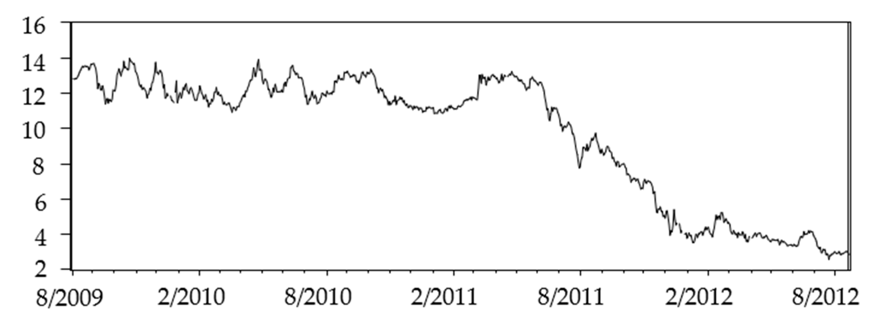
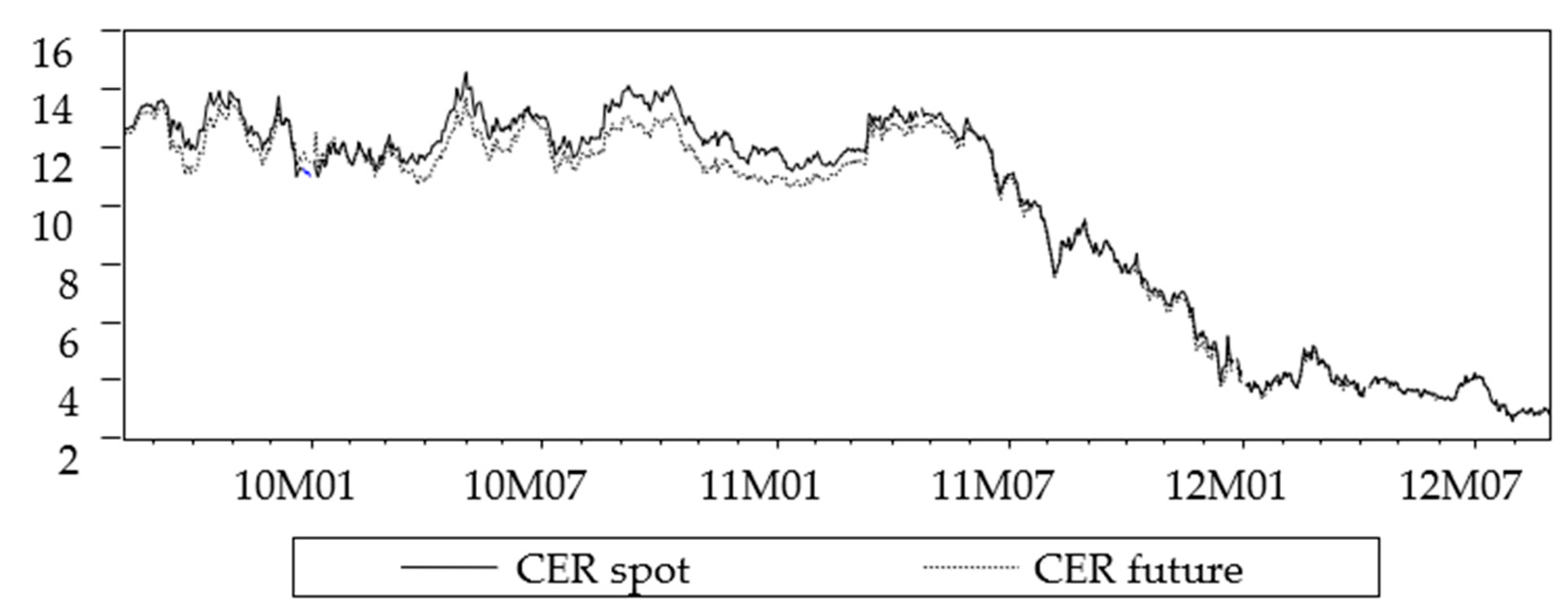
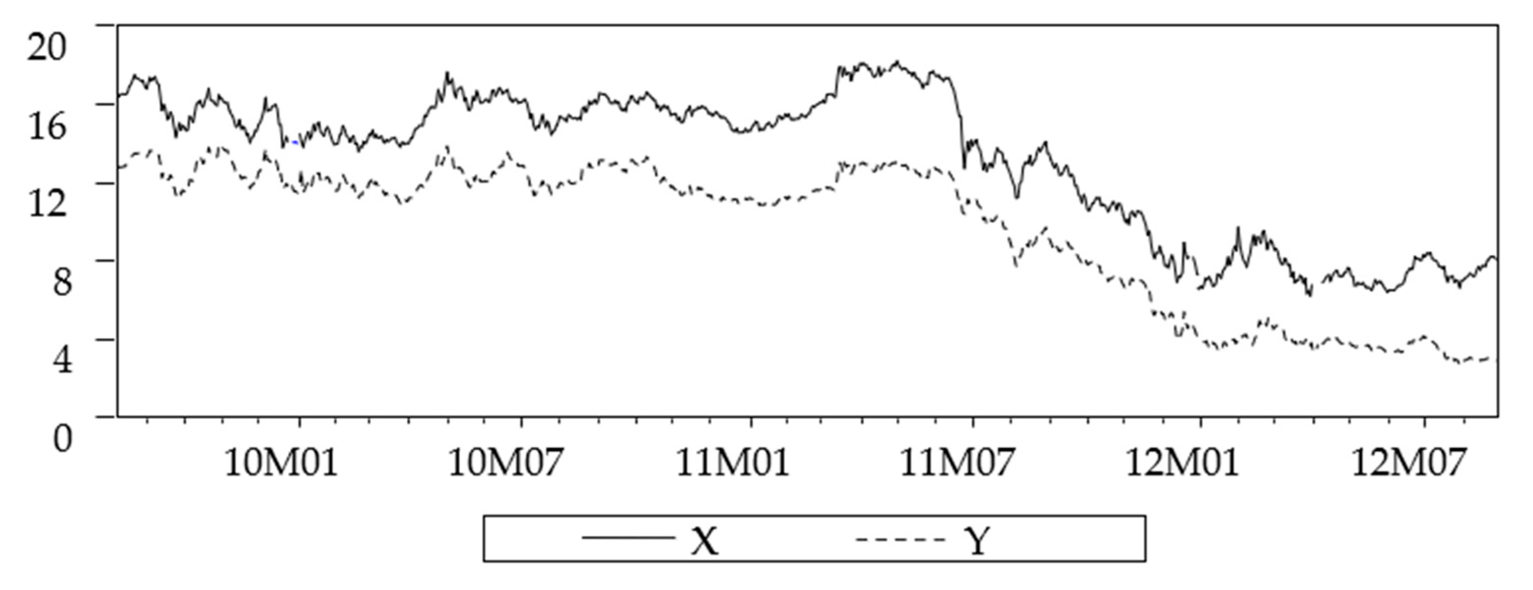
Taking the time series data of CER futures prices as an example, the ARIMA model was established to verify whether the model has a good prediction function for CER futures prices. Before the model construction, a CER futures price time series chart was drawn to make a prejudgment. The number of samples was 798, and the trend graph is shown in Figure 1:

According to Figure 1, the price of this series was in a stationary state before May 2011, but the price had a significant downward trend after June 2011. In general, the price showed a characteristic of volatility during the observation period, and it was initially judged that this series was nonstationary.

Before the ARIMA model was built, unit root test was carried out first. The purpose of unit root test is to test the stationarity of time series variables and avoid a pseudo regression of the model. Therefore, unit root test is very important, and the stationarity of time series is an important problem that must be considered when establishing a time series model. The reason why a unit root test is widely used is that most economic time series have a unit root after pair transformation. Currently, there are six methods for a unit root test: ADF (DF) test, PP test, DFGLS test, KPSS test, ERS test, and NP test. The widely used ADF test method was adopted in this paper.

If y_t has a p-order sequence correlation, the p-order autoregressive process can be used to correct the y_t. The model with trend term after it becomes stationary through difference is:

$${\Delta \mathrm{y}}_{\mathrm{t}}={\mathsf{\eta }\mathrm{y}}_{\mathrm{t}-1}+\mathrm{a}+\mathsf{\delta }\mathrm{t}+{\displaystyle \sum }_{\mathrm{i}=1}^{\mathrm{p}-1}{\mathsf{\beta }}_{\mathrm{i}\Delta }{\mathrm{y}}_{\mathrm{t}-\mathrm{i}}+{\mathrm{u}}_{\mathrm{t}} \left(\mathrm{t}=1,2,\cdots ,\mathrm{T}\right)$$

(4)

where, a is a constant term; δ_t is a linear trend function; and if η < 0, then y_t is stationary and if η = 0, then y_t has at least one unit root.

Using software Eviews 6.0 to carry out ADF test [33], the results are shown in

Table 1. ADF test results of the CER futures prices.

ADF Statistics			T Statistics	Probability Value p Value
			−0.120956	0.9452
Significance level	1%	test threshold	−3.438454
	5%		−2.865007
	10%		−2.568671

:

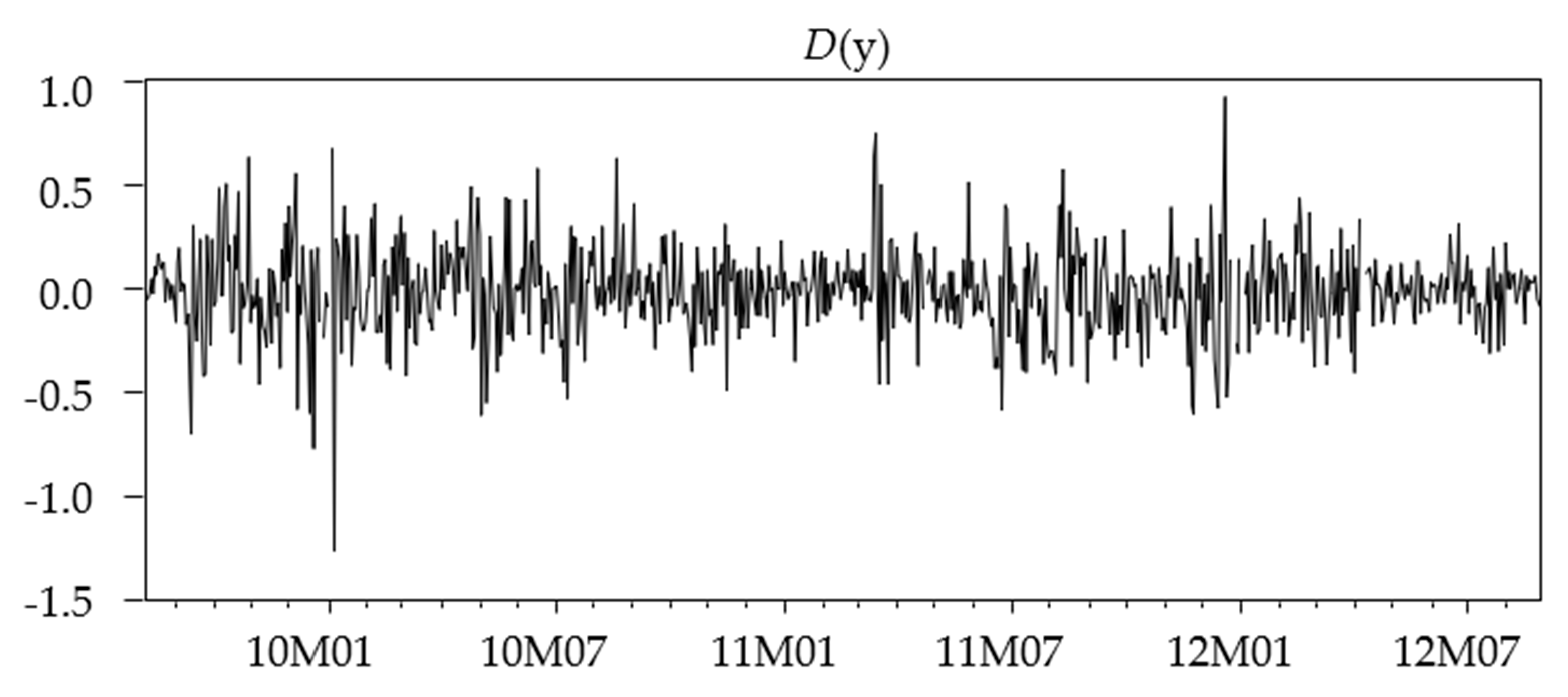
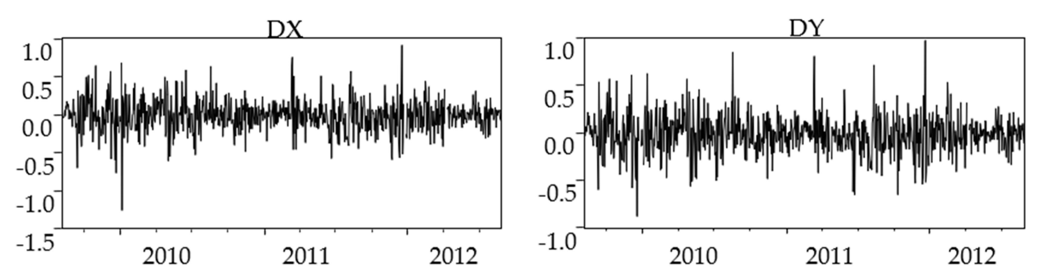
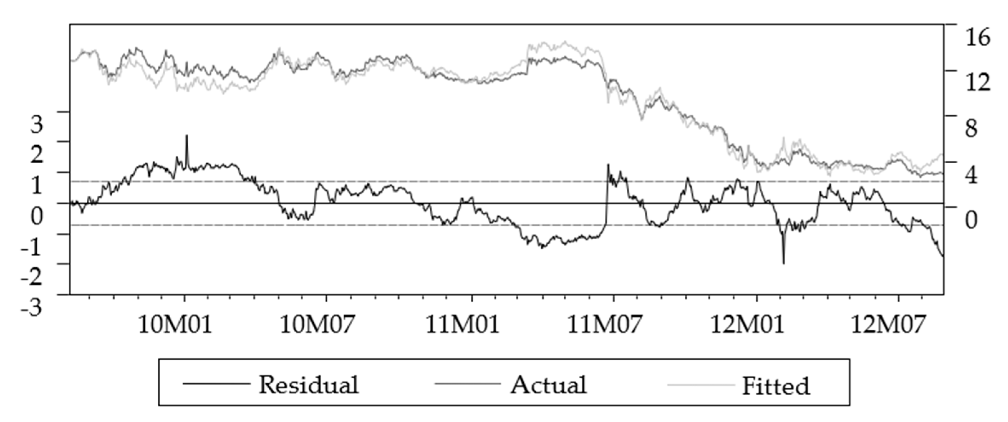
From the test results, under the three significance levels of 1%, 5%, and 10%, the MacKinnon critical values of the unit root test were −3.4385, −2.8650, and −2.5687, respectively, and the t-test statistics of −0.1210 was greater than the corresponding critical value, so H₀ could not be rejected, indicating that the CER futures price series had a unit root and was a nonstationary sequence. The first-order difference was applied to the CER futures price series, and the difference sequence is shown in Figure 2. From the difference sequence figure, it can be seen that a price downward trend of the original sequence was eliminated after the first-order difference, and the difference sequence showed stationarity.

Then, the ADF test with intercept term was carried out for D (y), and the lag order (p = 4) was determined by SIC criterion. The test results are shown in

Table 2. CER futures first-order difference D (y) unit root test results.

ADF Statistics			t Statistics	Probability Value p Value
			−28.91714	0.0000
Significance level	1%	test threshold	−3.438529
	5%		−2.865040
	10%		−2.568689

:

Table 2 shows that the t statistics value of D (y) was −28.9171, which was less than any value under the given significance level. Therefore, the original hypothesis was rejected and the difference sequence of CER futures price had no unit root and was a stationary sequence, that is, the Y sequence was integrated of order 1, Y~I(1).

3.2. Model Identification and Order Determination

The order of the model was estimated by autocorrelation and partial autocorrelation graphs. As shown in Figure 3, AC and PAC coefficients of D (y) correlation graphs were all tailing, and AC and PAC coefficients were obviously not 0 at the lag phases 18, 19, and 31, so p was set as 1, 2, 3, and q was set as 1, 2, 3. After multiple tests and a comprehensive comparison of AIC and SC values of multiple models, ARIMA (3,1,3) was finally determined to be more appropriate.

3.3. Parameter Estimation of the Model

Software Eviews6.0 was used to estimate parameters of the CER futures price model, and the estimated results of the model were:

$$\begin{array}{cc}\hfill {\mathrm{Dy}}_{\mathrm{t}}& =-0.0126-0.9309({\mathrm{Dy}}_{\mathrm{t}-3}+0.0126)+{\mathrm{u}}_{\mathrm{t}}-0.95{60\mathrm{u}}_{\mathrm{t}-3}\hfill \\ & =-0.0243-0.9309{\mathrm{Dy}}_{\mathrm{t}-3}+{\mathrm{u}}_{\mathrm{t}}-0.9560{\mathrm{u}}_{\mathrm{t}-3}\hfill \\ & \mathrm{t}=(-1.6592) (-21.0617) \left(26.9317\right)\hfill \\ & {\mathrm{R}}^2=0.0061 \mathrm{F}=2.4204 \mathrm{D}.\mathrm{W}.=2.0395\hfill \end{array}$$

(5)

3.4. Diagnosis and Test of Model

The model passed t-test, F-test, and D.W.-test. The reciprocal of the characteristic root was less than 1, indicating that the AR (1) and MA (1) models were reversible. The residual sequence correlation graph of the model is shown in Figure 4. It can be seen from Figure 4 that there was no autocorrelation of model residuals. When the lag phase K = 36, the Q statistics’ adjoint probability p = 0.114 > α = 0.05, indicating that the residual sequence of each order of the model was white noise. Therefore, Formula (5) was the best model.

3.5. Prediction of the Model

This paper took the CER futures price due in December 2012 of the European Climate Exchange (ECX) as the research object. The research period was from 7 August 2009 to 25 September 2012, with 818 samples in total [34]. A total of 798 samples from 7 August 2009 to 28 August 2012 were used for parameter estimation to predict trading prices in the next 20 trading days. Figure 5 shows the fitting of y_t and Formula (5) dynamic prediction value $\hat{\mathrm{y}}$_t.

As can be seen from the figure above, the predicted value of Formula (5) fit the actual value well, and it could be concluded that ARIMA, a single autoregressive integrated moving average model, had a good fitting and prediction effect on carbon emission trading prices, and had a certain practical guiding significance.

4. An Empirical Analysis of CER Futures Pricing Function in Carbon Financial Market

4.1. Correlation Analysis of Spot Price and Futures Price

Firstly, the sample range of the CER spot price and futures price trend graph (Figure 6) analyzed in this paper was from 7 August 2009 to 28 August 2012, with 798 samples in total.

As can be seen from Figure 6, trend and fluctuation of the CER futures price was strongly consistent with that of spot price. Software Eviews6.0 was used to process price data of the CER spot and futures, in which X represents time series of the CER futures price and Y represents time series of the CER spot price. Besides, the OLS method was used to estimate linear regression model of the spot price and futures price:

$$\begin{array}{c}{\mathrm{y}}_{\mathrm{t}}=-0.0939+1.0277{\mathrm{x}}_{\mathrm{t}}\\ \mathrm{t}=(-3.032981) \left(342.2911\right)\\ {\mathrm{R}}^2=0.9933 \mathrm{F}=117163.2 \mathrm{D}.\mathrm{W}.=0.1003.\end{array}$$

(6)

The coefficient of determination of the equation was high, and the regression coefficient was significant. For the model with 798 samples, using one explanatory variable and a 1% significance level, it can be seen from the D.W. statistical table that d_L = 1.664, d_U = 1.684, D.W. < D_L in the model, obviously indicating that there was autocorrelation in the price model. This can also be seen from the residual diagram, as shown in Figure 3, Figure 4, Figure 5, Figure 6 and Figure 7.

According to Figure 7, the fitting degree of the actual value and the fitting value was relatively high; that is, the CER futures price and the CER spot price had the same change trend and a high correlation, so that spot price could be analyzed and predicted through the futures price, showing a function of price discovery. In spite of this, some time series data tend to have a same trend of change. Even if two variables are not actually related, they may show a more significant “correlation”, which may lead to a pseudo regression. Meanwhile, the change mode of the residual showed that the residual was continuously positive and continuously negative, indicating that there was a first-order positive autocorrelation in the residual term and conclusions of t statistics and F statistics in the model were not credible, so remedial measures need to be taken.

4.2. Unit Root Test

As can be seen from Figure 6, trend graph of the CER spot and futures prices is not in a stationary state, and the ADF test, under SIC criterion, was conducted for the y and x series with constant terms respectively, and the test results are shown in

Table 3. CER spot price (Y) and futures prices (X) unit root test results.

Samples	ADF Test Statistics	1% Horizontal Critical Value	5% Horizontal Critical Value	10% Horizontal Critical Value
Y	−0.016579	−3.438454	−2.865007	−2.568671
X	−0.120956	−3.438454	−2.865007	−2.568671

.

According to Table 3, ADF test statistics of the y and x series were greater than the horizontal critical value, indicating that there were unit roots in the y and x series, and the series were both nonstationary. The difference method was applied to adjust the y and x series to stationary series. After a first-order difference, the trend graphs of y and x difference sequences showed a stationary trend, as shown in Figure 8.

Then, an ADF test, under SIC criterion, was conducted for the first-order difference sequence with constant terms, and the test results are shown in

Table 4. First-order differential sequence DY and DX unit root test results.

Samples	ADF Test Statistics	1% Horizontal Critical Value	5% Horizontal Critical Value	10% Horizontal Critical Value
DY	−27.84365	−3.438529	−2.865040	−2.568689
DX	−28.91714	−3.438529	−2.865040	−2.568689

. It can be seen from Table 4 that the t statistics values of D (y) and D (x) were less than any given value under the significance level. Therefore, the original hypothesis was rejected. The first-order difference sequences of the CER spot and futures prices did not have unit roots, which were stationary series, that is, both y and x sequences were integrated of order 1, Y~I(1).

After the first-order difference, the price series of the CER spot and future showed stationarity, and according to Figure 6, there was a long-term and consistent trend of change between the two series, showing a long-term stationary equilibrium relationship between them. Granger pointed out that if there is a co-integration relationship between two time series, then there is Granger causality between x and y in at least one direction.

4.3. Granger Causality Test

There are some variables that are significantly correlated within economic variables, but they are not necessarily all meaningful. It is a common problem in econometrics to determine whether a change in one variable is the cause of a change in another. Granger proposed a test to judge causality, which is called Granger causality test [35]. Granger solved the problem of whether x causes Y, mainly depending on the extent to which the current y can be explained by the past x, and on whether adding the lag value of x can improve the interpretation. If x is helpful in predicting y, or if the correlation coefficient between x and y is statistically significant, then it can be said that “y is caused by x Granger”.

The regression test formula of the Granger causality between ${\mathrm{x}}_{\mathrm{t}}$ and ${\mathrm{y}}_{\mathrm{t}}$ is expressed as follows:

$$\begin{array}{cc}\hfill {\mathrm{y}}_{\mathrm{t}}& ={\displaystyle {\displaystyle \sum }_{\mathrm{i}=1}^{\mathrm{k}}}{\mathsf{\alpha }}_{\mathrm{i}}{\mathrm{y}}_{\mathrm{t}-\mathrm{i}}+{\displaystyle {\displaystyle \sum }_{\mathrm{i}=1}^{\mathrm{k}}}{\mathsf{\beta }}_{\mathrm{i}}{\mathrm{x}}_{\mathrm{t}-\mathrm{i}}+{\mathrm{u}}_{1\mathrm{t}}\hfill \\ \hfill {\mathrm{x}}_{\mathrm{t}}& ={{\displaystyle \sum }}_{\mathrm{i}=1}^{\mathrm{k}}{\mathsf{\alpha }}_{\mathrm{i}}{\mathrm{x}}_{\mathrm{t}-\mathrm{i}}+{{\displaystyle \sum }}_{\mathrm{i}=1}^{\mathrm{k}}{\mathsf{\beta }}_{\mathrm{i}}{\mathrm{y}}_{\mathrm{t}-\mathrm{i}}+{\mathrm{u}}_{2\mathrm{t}}.\hfill \end{array}$$

(7)

The original hypothesis to test that there is no Granger causality between x_t−1 and y_t is

H₀: β₁ = β₂ = … β_k = 0.

If the estimated values of regression parameters of lag variables of ${\mathrm{x}}_{\mathrm{t}}$ in Formula (7) are all not significant, then the above hypothesis cannot be rejected. In other words, if the estimated value of regression parameters of any lagged variable of x_t is significant (not equal to 0), the conclusion should be that there is Granger causality between x_t−1 and y_t. The above tests can be done with F statistics.

$$\mathrm{F}=\frac{\left({\mathrm{RSS}}_{\mathrm{r}}-{\mathrm{RSS}}_{\mathrm{u}}\right)/\mathrm{k}}{{\mathrm{RSS}}_{\mathrm{u}}/\left(\mathrm{T}-2\mathrm{k}\right)}$$

(8)

where, RSS_r is sum of squares of the model residuals after a constraint is applied, and RSS_u represents sum of squares of the model residuals without constraints; k represents the maximum lag of x_t in the model, 2k represents the number of estimated parameters in the unconstrained model, and T is the sample size.

Under the condition that the null hypothesis is true, F statistics asymptotically follow the F_α (k, T − 2k) distribution. If F ≤ F_α (k, T − 2k), calculated with the samples, then accept the null hypothesis, that is, there is no Granger causality between x_t−1 and y_t. If F > F_α (k, T − 2k), calculated with the samples, then reject the null hypothesis, that is, there is Granger causality between x_t−1 and y_t. Since the null hypothesis of the hypothesis test has no causality, F statistics, under this hypothesis, follows F distribution, so strictly speaking, this test should be called Granger causality test.

The two groups of series were formed into an array for the Granger causality test as there is a co-integration relationship between the CER spot price series and the CER futures price series. Due to the daily price data used, the frequency of change was high, and it took a certain time to affect the transmission, so a more comprehensive Granger causality could be found by adjusting the lag period. The test results are shown in

Table 5. CER spot and futures prices Granger causality test results.

Lag Divisor	Y Does not Granger Cause X			X Does not Granger Cause Y
	F Value	p Value	Conclusion	F Value	p Value	Conclusion
1	7.8242	0.0053	Reject the null hypothesis	0.62984	0.4277	Accept the null hypothesis
2	6.6728	0.0013	Reject the null hypothesis	1.9079	0.1377	Accept the null hypothesis
3	1.3936	0.2435	Accept the null hypothesis	2.2037	0.0863	Accept the null hypothesis
4	1.1347	0.3389	Accept the null hypothesis	2.3302	0.0546	Accept the null hypothesis
5	1.3479	0.2421	Accept the null hypothesis	2.2024	0.0523	Accept the null hypothesis
10	1.0705	0.3826	Accept the null hypothesis	1.4347	0.1604	Accept the null hypothesis

.

As can be seen from Table 5, the CER spot price, under the condition that the lag period was 1 or 2, was the Granger cause of the CER futures price, while the CER futures price was not the Granger cause of the CER spot price. There was no Granger causality between CER spot price and CER futures price after the third lag phase, showing that the CER market is not mature, and the CER future price cannot reflect the price discovery function. On the contrary, it is the spot price that guides the future price. The main reason is that the carbon trading market is greatly influenced by the policies of various countries, and there are many uncertain factors in the carbon trading itself. As the end time of the first commitment period of the Kyoto Protocol in 2012 approaches, there is no agreement on the future trading policy, which leads to the inability of investors to accurately predict the future investment, which greatly affects the carbon market under the condition of perfect competition and hinders the sound development of the carbon market.

4.4. Co-Integration Test and Correcting the Model with ECM Error

In this paper, the Engle–Granger (EG) test method proposed by Engle and Granger in 1987 was adopted [36]. The Granger theorem links ECM, that is, there must be an ECM expression for a first-order integral variable with a co-integration relationship.

According to the requirements of co-integration theory, CER spot prices and CER futures prices are both sequences of first-order integration, with the same single-order integration number. Therefore, firstly, linear regression models of the two were estimated by OLS regression method:

$$\begin{array}{c}{\mathrm{y}}_{\mathrm{t}}=-0.0939+1.0277{\mathrm{x}}_{\mathrm{t}}+{\mathrm{e}}_{\mathrm{t}}\\ \mathrm{t}=(-3.032981) \left(342.2911\right)\\ {\mathrm{R}}^2=0.9933 \mathrm{F}=117163.2 \mathrm{D}.\mathrm{W}.=0.1003.\end{array}$$

(9)

Secondly, the unit root test was carried out for residuals of the above formula with no intercept term and time trend term. The test results of the lag order determined by SIC criterion are shown in

Table 6. Residual series unit root test results.

ADF Statistics			t Statistics	Probability Value p Value
			−4.514333	0.0002
Significance level	1%	test threshold	−3.438529
	5%		−2.865040
	10%		−2.568689

below:

Test results show that the sequence rejected the null hypothesis at 1% significance level, so e_t so could be determined as a stationary sequence, i.e., e_t ~ I (0). The above results show that there was a long-term co-integration relationship between the CER spot price and the CER futures price from 7 August 2009 to 28 August 2012, which was CI (1,1), and the co-integration vector was (1, −1.0277). However, in the short term, there may be imbalances. In order to enhance accuracy of the model, the error term e_t in the above co-integration regression could be regarded as an equilibrium error. By establishing ECM, the short-term behavior of spot price can be linked with a long-term change.

According to the two-step method of ECM EG, the first step calculating the co-integration regression model has been completed, and then the second step takes the residual sequence as an error correction term to establish ECM, and the regression model is as follow:

$${\Delta \mathrm{y}}_{\mathrm{t}}=\mathsf{\alpha }+{\mathsf{\gamma }}_0{\Delta \mathrm{x}}_{\mathrm{t}}+{\mathsf{\delta }}_1{\mathrm{e}}_{\mathrm{t}-1}+{\mathrm{u}}_{\mathrm{t}}.$$

Estimated regression model:

$$\begin{array}{c}\Delta {\mathrm{y}}_{\mathrm{t}}=-0.0017+0.8775{\Delta \mathrm{x}}_{\mathrm{t}}-0.0414{\mathrm{e}}_{\mathrm{t}-1}\\ \mathrm{t}=(-0.5289) \left(56.9150\right) (-3.8827)\\ {\mathrm{R}}^2=0.8057 \mathrm{F}=1621.257 \mathrm{D}.\mathrm{W}.=2.426.\end{array}$$

(10)

The above estimating results show that the change of CER spot price depends not only on the change of CER futures price, but also on the deviation of previous CER spot price to the equilibrium level. The difference term reflects the influence of short-term fluctuations. Short-term fluctuations of CER spot price can be divided into two parts: one is the impact of short-term CER futures price fluctuations and the other is the effect of CER spot price deviating from long-term equilibrium. The estimating coefficient (−0.0414) of the error term e_t−1 reflects a correction of the deviation. When the short-term fluctuation deviates from the long-term equilibrium, it will pull the unbalanced state back to an equilibrium state with the adjustment force of (−0.01414).

5. An Empirical Analysis of the EUA Futures Prices and CER Futures Prices in the Carbon Financial Market

In the carbon trading market, in addition to the price discovery function in the CER market, there is also a dynamic linkage relationship between EUA market and CER market. This paper, taking the EUA futures contract price data and CER futures contract price data, due in December 2012, as samples [37], analyzed the linkage relationship between futures prices of the two markets from 7 August 2009 to 28 August 2012.

5.1. Correlation Analysis of EUA Futures Price and CER Futures Price

Firstly, the sample range of the EUA futures price and CER futures price trend graph (Figure 9) analyzed in this paper was from 7 August 2009 to 28 August 2012, with 798 samples in total.

As can be seen from the figure above, trend and fluctuation of the EUA futures price was strongly consistent with that of the CER futures price. Using software Eviews6.0 to process price data of the CER spot and futures, where X represents time series of the CER futures price, Y represents time series of the CER spot price, and OLS method was used to estimate linear regression model of the spot price and futures price:

$$\begin{array}{c}{\mathrm{y}}_{\mathrm{t}}=-3.2734+0.9764{\mathrm{x}}_{\mathrm{t}}\\ \mathrm{t}=(-33.9998) \left(139.1935\right)\\ {\mathrm{R}}^2=0.9608 \mathrm{F}=19374.84 \mathrm{D}.\mathrm{W}.=0.0379.\end{array}$$

(11)

Coefficient of determination of the equation was high, and the regression coefficient was significant. For the model with 798 samples, with one explanatory variable and 1% significance level, it can be seen from the D.W. statistical table that d_L = 1.664, d_U = 1.684, D.W. < d_L in the model, obviously indicating that there was autocorrelation in the price model. This can also be seen from the residual diagram, as shown in Figure 10.

As can be seen from Figure 10, fitting degree of the actual value and the fitting value was relatively high, that is, the CER futures price and the EUA futures price had the same change trend and a high correlation, so that CER futures price can be analyzed and predicted through EUA futures price, showing a function of price discovery. In spite of this, some time series data tend to have the same trend of change. Even if two variables are not actually related, they may show a more significant “correlation”, which may lead to a pseudo regression. Meanwhile, change mode of the residual showed that the residual was continuously positive and continuously negative, indicating that there was a first-order positive autocorrelation in the residual term, and conclusions of t statistics and F statistics in the model were not credible, so remedial measures need to be taken.

5.2. Unit Root Test

As can be seen from Figure 10, the trend graph of the CER futures price and the EUA futures price were not in a stationary state, and ADF test, under SIC criterion with lag phase of 4 (p = 4), needed to be conducted for the y and x series with constant terms respectively, and the test results are shown in

Table 7. CER futures(Y) and EUA futures (X) prices unit root test results.

Sample	ADF Test Statistics	1% Horizontal Critical Value	5% Horizontal Critical Value	10% Horizontal Critical Value
Y	−0.221769	−3.438739	−2.865132	−2.568738
X	−0.998438	−3.438739	−2.865132	−2.568738

.

According to Table 7, ADF test statistics of the y and x series were greater than the horizontal critical value, indicating that there were unit roots in the y and x series, and the series were all nonstationary. The difference method was applied to adjust y and x series to stationary series. After a first-order difference, the trend graphs of y and x difference sequences showed a stationary trend, as shown in Figure 11.

Then, an ADF test under SIC criterion was conducted for the first-order difference sequence with constant terms, and the test results are shown in

Table 8. The first-order differential sequence DY and DX unit root test results.

Samples	ADF Test Statistics	1% Horizontal Critical Value	5% Horizontal Critical Value	10% Horizontal Critical Value
DY	−12.11232	−3.438796	−2.865158	−2.568752
DX	−12.53168	−3.438796	−2.865158	−2.568752

. It can be seen from Table 8 that the t statistics values of D (y) and D (x) were less than any given value under the significance level. Therefore, the original hypothesis was rejected. The first-order difference sequences of the EUA futures prices and CER futures prices did not have unit roots, which were stationary series, that is, both y and x sequences were integrated of order 1, Y~I(1).

It can be seen from Table 2 that the t statistics value of D (y) was −28.9171, which was less than any value under the given significance level. Therefore, the original hypothesis was rejected, and the difference sequence of CER futures price had no unit root and was a stationary sequence, that is, the Y sequence was integrated of order 1, Y~I(1).

After a first-order difference, the EUA futures price and CER futures price series showed the stationarity, and according to Figure 11, there was a long-term and consistent trend of change between the two series, showing a long-term stationary equilibrium relationship between them. Granger pointed out that if there is a co-integration relationship between two time series, then there is Granger causality x and y in at least one direction.

5.3. Granger Causality Test

The two groups of series were formed into an array for the Granger causality test as there was a co-integration relationship between the EUA futures price series and the CER futures price series. Due to the daily price data used, the frequency of change was high, and it took a certain time to affect the transmission, so a more comprehensive Granger causality (see

Table 9. CER spot and future prices Granger causality test results.

Lag Order	Y Does Not Granger Cause X			X Does Not Granger Cause Y
	F Value	p Value	Conclusion	F Value	p Value	Conclusion
1	1.5564	0.2126	Accept the null hypothesis	0.0177	0.8942	Accept the null hypothesis
2	0.8719	0.4186	Accept the null hypothesis	0.1454	0.8647	Accept the null hypothesis
3	2.1881	0.0881	Accept the null hypothesis	3.3056	0.0198	Reject the null
4	1.8905	0.1102	Accept the null hypothesis	2.7779	0.0261	Reject the null
5	2.1690	0.0557	Accept the null hypothesis	2.8298	0.0153	Reject the null
10	1.3329	0.2085	Accept the null hypothesis	1.5317	0.1236	Accept the null hypothesis
15	1.1667	0.2930	Accept the null hypothesis	1.2856	0.2050	Accept the null hypothesis

) could be found by adjusting the lag period.

As can be seen from Table 9, the EUA futures price, under the condition that the lag period was 3–5, was the Granger cause of the CER futures price, but the CER futures price was not the Granger cause of the EUA futures price. There was no Granger causality between EUA futures price and CER futures price after the fifth lag phase, showing that there was not a long-term Granger causality between the EUA futures market and the CER futures market, the EUA futures price could, in the short term, reflect the price discovery function on the CER futures price, but with the extension of the lag order, the influence of the EUA futures price on the CER futures price was gradually weakened. The reason is that, on the whole, the operation and scale of the EUA market are much larger than that of the CER market, which has a wide influence and plays a leading role in achieving global carbon emission reduction. Therefore, the carbon price in the EUA market can better reflect the price discovery function than the carbon price in the CER market. However, the EUA market price cannot, in the long run, guide the CER market price as they are not highly interdependent, though the two markets have differentiation between what is primary and what is secondary. It is also related to their different policy orientations and the determination of the future development direction. The EUA market policy is relatively clear, but many factors, such as the CER market policy arrangement after 2012, are not clear, so the effect of using the price mechanism to reflect the real market situation is not obvious. With the continuous improvement of the policy, the two market prices will be able to better reflect the real information of financial products.

5.4. Co-Integration Test and ECM

According to the requirements of co-integration theory, EUA futures prices and CER futures prices are both sequences of first-order integration, with the same single-order integration number. Therefore, firstly, linear regression models of the two were estimated by OLS regression method:

$$\begin{array}{c}{\mathrm{y}}_{\mathrm{t}}=-3.2734+0.9764{\mathrm{x}}_{\mathrm{t}}+{\mathrm{e}}_{\mathrm{t}}\\ \mathrm{t}=(-33.9998) \left(139.1935\right)\\ {\mathrm{R}}^2=0.9608 \mathrm{F}=19374.84 \mathrm{D}.\mathrm{W}.=0.0379.\end{array}$$

(12)

Secondly, the unit root test was carried out for residuals of the above formula with no intercept term and time trend term. The test results of the lag order determined by SIC criterion are shown in

Table 10. Residual series units root test results.

ADF Statistics			t Statistics	Probability Value p Value
			−2.321855	0.0196
Significance level	1%	Test threshold	−2.567911
	5%		−1.941227
	10%		−1.616428

below:

Test results show that the sequence rejected the null hypothesis at 5% significance level, so it was determined e_t to be a stationary sequence, i.e., e_t ~ I (0). The above results show that there was a long-term co-integration relationship between the EUA futures price and the CER futures price from 7 August 2009 to 28 August 2012, which was CI (1,1), and the co-integration vector was (1, −0.9764). However, there may have been imbalances in the short term. In order to enhance accuracy of the model, the error term e_t in the above co-integration regression could be regarded as an equilibrium error. Through the establishment of ECM, the short-term behavior of spot price can be linked with a long-term change.

According to the two-step method of ECMEG, the first step calculating the co-integration regression model was completed, and then the second step took the residual sequence as an error correction term to establish ECM, and the regression model was obtained by estimating:

$$\begin{array}{c}{\Delta \mathrm{y}}_{\mathrm{t}}=-0.0060+0.6467{\Delta \mathrm{x}}_{\mathrm{t}}-0.0103{\mathrm{e}}_{\mathrm{t}-1}\\ \mathrm{t}=(-1.6202) \left(49.6887\right) (-1.9975)\\ {\mathrm{R}}^2=0.7595 \mathrm{F}=1234.506 \mathrm{D}.\mathrm{W}.=2.0679.\end{array}$$

(13)

The above estimation results show that the change of CER futures price depends not only on the change of EUA futures price, but also on the deviation of previous CER futures price to the equilibrium level. The difference term reflects the influence of short-term fluctuations. Short-term fluctuations of CER futures prices can be divided into two parts: one is the impact of short-term EUA futures price fluctuations and the other is the effect of CER futures and EUA futures deviating from long-term equilibrium. The estimating coefficient (−0.0103) of the error term e_t−1 reflects a correction of the deviation. When the short-term fluctuation deviates from the long-term equilibrium, it will pull the unbalanced state back to an equilibrium state with the adjustment force of (−0.0103).

6. Conclusions

In the Guide to Chinese Climate Policy 2019, Chinese leaders declared that the impact of climate change “poses a great challenge to human survival and development” and that China is “one of the countries most vulnerable to the adverse effects of climate change”. China is one of the countries hardest hit by climate change, so its active response to climate change is an intrinsic requirement for China to achieve sustainable development and they have a responsibility to promote the common development of all humankind [38,39,40]. Therefore, China is actively establishing a carbon financial market, with spot trading as the main mode of carbon trading, while the carbon futures market is only at the stage of preliminary ideas [41,42,43]. Given that China’s carbon trading market is at the end of the international carbon trading market, and the market trading lacks power of discourse and pricing, this paper, in order to change the current situation and improve the international status of China’s carbon trading, introduced the future pricing mechanism into the carbon trading process, hoping to play a positive role in the establishment of pricing mechanism of carbon financial market in China [44,45]. This paper took futures price data of the European Climate Exchange and spot price data of the BlueNext environment exchange as samples, and made an empirical analysis on the change relationship between current EUA futures price and CER futures price, the change relationship between CER futures price and CER spot price, as well as the influencing factors of price fluctuation [46]. The following conclusions have been drawn from the introduction of the futures pricing mechanism:

(1) The price discovery function in the futures pricing mechanism should have not been formed in the CDM market. On the one hand, this confirms the fact that the trading volume of the clean development mechanism (CDM) project market accounts for less than 20% of the global carbon market. The immaturity of market development and the imperfection of the system, rules, and system are the fundamental reasons for this result. On the other hand, it also reflects that the market is greatly influenced by the government’s macro policies, which greatly influences the formation of the price mechanism under the condition of perfect competition in the carbon market and hinders the benign development of the carbon market.

(2) After the relationship between futures price changes between the EU allowances market and the clean development mechanism (CDM) project market in the short term was analyzed, it was found that the price discovery function of the futures pricing mechanism has been preliminarily formed. EUA futures prices can influence the trend of CER prices in the CDM market. In the long run, the EUA futures price in the EU allowances market has less and less influence on the CER futures price in the CDM market. The price discovery function of futures pricing is not obvious or is virtually nonexistent. On the one hand, it proves that the operation and scale of the EU allowances market are much larger than that of the CDM market, which has a wide influence and plays a leading role in realizing global carbon emission reduction. In addition, it also reflects that the futures prices in the EU allowances market cannot guide the futures prices in the CER market in the long run as they are not highly interdependent, though the two markets have differentiation between what is primary and what is secondary. It is also related to the different policy orientations of the two markets and the determination of the future development direction. The EUA market policy is relatively clear, but many factors, such as the CER market policy arrangement after 2012, are not clear. As a consequence, the effect of using the price mechanism to reflect the real market situation is insignificant. With the continuous improvement of policies, however, the two market prices will be able to better reflect real information of financial products.

7. Limitations and Influence of Research

In the process of studying the futures pricing mechanism of China’s carbon financial market, there are some limitations that arose in the research scope and research methods, which may have a certain influence on the establishment of China’s carbon financial market pricing mechanism. Firstly, in terms of research scope, this paper used the ARIMA model to select the settlement price data of EUA and CER futures due in December 2012 from ECX, and selected the spot settlement price data of EUA and CER from BlueNext environment exchange as research samples. The reason why the 2012 data were selected as the sample was that the establishment of carbon financial market in China was in the initial stage, and the data of ECX and BlueNext environment exchange should be used as reference. However, since the international carbon financial market is greatly influenced by policies in the initial stage, the data are strongly interfered with by human factors and the market lacks activity. So it is likely to lead to a decline in the guidance of the research conclusions on the establishment of China’s carbon price mechanism. Secondly, in terms of research methods, the ARIMA model was selected to analyze carbon price. Due to its simplicity, feasibility, and flexibility, the ARIMA model is widely used in financial time series, and it can achieve reasonable prediction of carbon prices. However, when dealing with the fluctuation of carbon price, which is influenced by complex and diversified factors, many objects and methods of prediction are used. It is difficult to describe the case with an accurate mathematical model, and the ARIMA model cannot meet the requirements of prediction accuracy. Therefore, in the process of carbon price research, we can consider the introduction of artificial neural network technology to build a prediction model to improve the prediction accuracy in the future.

References

1. Cervelló-Royo, R.; Moya-Clemente, I.; Perelló-Marín, M.R.; Ribes-Giner, G. Sustainable development, economic and financial factors, that influence the opportunity-driven entrepreneurship. An fsQCA approach. J. Bus. Res. 2020, 115, 393–402. [Google Scholar] [CrossRef]
2. Ucal, M.; Xydis, G. Multidirectional Relationship between Energy Resources, Climate Changes and Sustainable development: Technoeconomic Analysis. Sustain. Cities Soc. 2020, 60, 1022. [Google Scholar] [CrossRef]
3. Galindo-Martín, M.A.; Castaño-Martínez, M.S.; Méndez-Picazo, M.T. The Relationship between Green Innovation, Social Entrepreneurship, and Sustainable Development. Sustainability 2020, 12, 4467. [Google Scholar] [CrossRef]
4. Kaku, K. An Inconvenient Truth-Global Warming on Greenhouse Gas (GHG) Reduction under Kyoto Protocol Regime to Post Kyoto Protocol in ASIA. Proc. Eng. 2011, 8, 515–519. [Google Scholar] [CrossRef] [Green Version]
5. Dai, E.; Yin, L.; Wang, Y.; Ma, L.; Tong, M. Quantitative Assessment of the Relative Impacts of Land Use and Climate Change on the Key Ecosystem Services in the Hengduan Mountain Region, China. Sustainability 2020, 12, 4100. [Google Scholar] [CrossRef]
6. Miyamoto, M.; Takeuchi, K. Climate agreement and technology diffusion: Impact of the Kyoto Protocol on international patent applications for renewable energy technologies. Energy Policy 2019, 129, 1331–1338. [Google Scholar] [CrossRef] [Green Version]
7. Lau, L.C.; Lee, K.T.; Mohamed, A.R. Global warming mitigation and renewable energy policy development from the Kyoto Protocol to the Copenhagen Accord—A comment. Renew. Sustain. Energy Rev. 2012, 16, 5280–5284. [Google Scholar] [CrossRef]
8. The World Bank. State and Trends of the Carbon Market 2010. Available online: https://documents.worldbank.org/en/publication/documents-reports/documentdetail/992381468155705390/state-and-trends-of-the-carbon-market-2010 (accessed on 7 September 2020).
9. Adedoyin, F.; Ozturk, I.; Abubakar, I.; Kumeka, T.; Folarin, O.; Bekun, F.V. Structural breaks in CO2 emissions: Are they caused by climate change protests or other factors? J. Environ. Manag. 2020, 266, 110628. [Google Scholar] [CrossRef]
10. Munir, Q.; Lean, H.H.; Smyth, R. CO2 emissions, energy consumption and economic growth in the ASEAN-5 countries: A cross-sectional dependence approach. Energy Econ. 2020, 85, 104571. [Google Scholar] [CrossRef]
11. Kang, S.H.; Islam, F.; Tiwari, A.K. The dynamic relationships among CO2 emissions, renewable and non-renewable energy sources, and economic growth in India: Evidence from time-varying Bayesian VAR model. Struct. Chang. Econ. Dyn. 2019, 50, 90–101. [Google Scholar] [CrossRef]
12. Jeong, K.; Hong, T.; Kim, J. Development of a CO2 emission benchmark for achieving the national CO2 emission reduction target by 2030. Energy Build. 2018, 1581, 86–94. [Google Scholar] [CrossRef]
13. Kossoy, A.; Guigon, P. State and Trends of the Carbon Market 2012; The World Bank: Washington, DC, USA, 2012. [Google Scholar]
14. Chunguang, S.; Degang, Z.; Guangyu, W.; Yingli, H. Research on risk mechanism of China ’s carbon financial market development from the perspective of ecological civilization. J. Comput. Appl. Math. 2021, 381, 112990. [Google Scholar]
15. Mansanet-Bataller, M.; Chevallier, J.; Hervé-Mignucci, M.; Alberola, E. EUA and sCER phase II price drivers: Unveiling the reasons for the existence of the EUA–sCER spread. Energy Policy 2011, 39, 1056–1069. [Google Scholar] [CrossRef] [Green Version]
16. Xu, J.; Deng, Y.; Shi, Y.; Huang, Y. A bi-level optimization approach for sustainable development and carbon emissions reduction towards construction materials industry: A case study from China. Sustain. Cities Soc. 2020, 53, 101828. [Google Scholar] [CrossRef]
17. Feng, L. Carbon Emissions Trading Market from the Perspective of Low Carbon Economy Strategy. J. Sichuan Univ. Sci. Eng. Soc. Sci. Ed. 2020, 35, 53–69. [Google Scholar]
18. Qin, Q.; He, H.; Li, L.; He, L. A Novel decomposition-ensemble based carbon price forecasting model integrated with local polynomial prediction. Comput. Econ. 2020, 55, 1249–1273. [Google Scholar] [CrossRef]
19. Chen, X. Prediction of stock-price based on ARIMA model and neural network model. J. Quant. Econ. 2017, 34, 30–34. [Google Scholar]
20. Lee, C.; Ku, S.; Cho, P.; Chang, W. Explaining future market return and evaluating market condition with common preferred spread index. Phys. A Stat. Mech. Appl. 2019, 5251, 921–934. [Google Scholar] [CrossRef]
21. Gärling, T.; Gamble, A. Perceived inflation and expected future prices in different currencies. J. Econ. Psychol. 2008, 29, 401–416. [Google Scholar] [CrossRef]
22. Kuriyama, A.; Abe, N. Ex-post assessment of the Kyoto Protocol—Quantification of CO2 mitigation impact in both Annex B and non-Annex B countries. Appl. Energy. 2018, 22015, 286–295. [Google Scholar] [CrossRef]
23. Lambe, F.; Jürisoo, M.; Lee, C.; Johnson, O. Can carbon finance transform household energy markets? A review of cookstove projects and programs in Kenya. Energy Res. Soc. Sci. 2015, 5, 55–66. [Google Scholar] [CrossRef]
24. Chevallier, J. Macroeconomics, finance, commodities: Interactions with carbon markets in a data-rich model. Econ. Model. 2011, 28, 557–567. [Google Scholar] [CrossRef] [Green Version]
25. Zhou, K.; Li, Y. Carbon finance and carbon market in China: Progress and challenges. J. Clean. Product. 2019, 3, 536–549. [Google Scholar] [CrossRef]
26. Box, G.E.P.; Jenkins, G.M. Time Series Analysis, Forecasting and Control, 2nd ed.; Holden-Day: San Francisco, CA, USA, 1976. [Google Scholar]
27. Stefan, M.; Wellenreuther, C. London vs. Leipzig: Price discovery of carbon futures during Phase III of the ETS. Econ. Lett. 2020, 188, 108990. [Google Scholar] [CrossRef] [Green Version]
28. European Commission. Directive 2003/87/EC Annex III. Available online: https://eur-lex.europa.eu/LexUriServ/LexUriServ.do?uri=OJ:L:2003:275:0032:0046:en:PDF (accessed on 7 September 2020).
29. ICE. Futures Europe Monthly Utility Markets Report-June 2012. Available online: https://www.theice.com/marketdata/reports/7/product/390/hub/564/isOption/false/isSpread/false (accessed on 7 September 2020).
30. ICE. ICE ECX EUA Futures. Available online: https://www.theice.com/products/197/EUA-Futures (accessed on 7 September 2020).
31. ICE. ICE ECX CER Futures. Available online: https://www.theice.com/products/814666/CER-Futures (accessed on 7 September 2020).
32. Gao, T. Econometric Analysis Methods and Modeling; Tsinghua University Press: Beijing, China, 2009; pp. 267–300. [Google Scholar]
33. Kapoor, N.; Ghosh, S. Long-term association between European and Indian markets on carbon credit price. Renew. Sustain. Energy Rev. 2014, 38, 656–662. [Google Scholar] [CrossRef]
34. Granger, C.W.J. Investigating causal relations by econometric models and cross-spectral methods. Econometrica 1969, 37, 424–438. [Google Scholar] [CrossRef]
35. Engle, R.F.; Granger, C.W.J. Cointegration and error correction: Representation, estimation, and testing. Econometrica 1987, 55, 251–276. [Google Scholar] [CrossRef]
36. Wang, Y.; Pan, J.; Pei, R.; Yang, G.; Yi, B. A Framework for Assessing Green Capacity Utilization Considering CO2 Emissions in China’s High-Tech Manufacturing Industry. Sustainability 2020, 12, 4424. [Google Scholar] [CrossRef]
37. Fragkos, P.; Tasios, N.; Paroussos, L.; Capros, P.; Tsani, S. Energy system impacts and policy implications of the European Intended Nationally Determined Contributions and low-carbon pathway to 2050. Energy Policy 2017, 100, 216–226. [Google Scholar] [CrossRef]
38. Xing, R.; Hanaoka, T.; Kanamori, Y.; Masui, T. Achieving China’s Intended Nationally Determined Contributions and its co-benefits: Effects of the residential sector. J. Clean. Prod. 2018, 17220, 2964–2977. [Google Scholar] [CrossRef]
39. Yang, X.; Song, Y.; Sun, M.; Peng, H. Strategies for Capital Constrained Timber and Carbon Sink Supply Chain under the Cap-and-Trade Scheme. Sustainability 2020, 12, 4380. [Google Scholar] [CrossRef]
40. Peng, B.; Tong, X.; Cao, S.; Li, W.; Xu, G. Carbon Emission Calculation Method and Low-Carbon Technology for Use in Expressway Construction. Sustainability 2020, 12, 3219. [Google Scholar] [CrossRef] [Green Version]
41. Finon, D. Carbon policy in developing countries: Giving priority to non-price instruments. Energy Policy 2019, 132, 38–43. [Google Scholar] [CrossRef]
42. Brown, D.P.; Eckert, A.; Eckert, H. Carbon pricing with an output subsidy under imperfect competition: The case of Alberta’s restructured electricity market. Resour. Energy Econ. 2018, 52, 102–123. [Google Scholar] [CrossRef] [Green Version]
43. Shen, C.-W.; Min, C.; Wang, C.-C. Analyzing the trend of O2O commerce by bilingual text mining on social media. Comput. Hum. Behav. 2019, 101, 474–483. [Google Scholar] [CrossRef]
44. Yan, X.; Chen, M.; Chen, M.-Y. Coupling and Coordination Development of Australian Energy, Economy, and Ecological Environment Systems from 2007 to 2016. Sustainability 2019, 11, 6568. [Google Scholar] [CrossRef] [Green Version]
45. Feng, B.; Sun, K.; Chen, M.; Gao, T. The Impact of Core Technological Capabilities of High-Tech Industry on Sustainable Competitive Advantage. Sustainability 2020, 12, 2980. [Google Scholar] [CrossRef] [Green Version]
46. Su, Y.; Han, L.; Wang, J.; Wang, H. Quantum-behaved RS-PSO-LSSVM method for quality prediction in parts production processes. Concurr. Comput. Pract. Exp. 2019, 9, e5522. [Google Scholar]
Figure 1. Certified Emission Reduction (CER) futures price trend graph.
Sustainability 12 07317 g001
Figure 2. CER futures price of a first-order differential sequence diagram.
Sustainability 12 07317 g002
Figure 3. CER futures first-order differential correlation diagram.
Sustainability 12 07317 g003
Figure 4. Residuals autocorrelation and partial autocorrelation diagram.
Sustainability 12 07317 g004
Figure 5. Fit figure of actual and predicted values.
Sustainability 12 07317 g005
Figure 6. Trend graph of CER spot and futures price.
Sustainability 12 07317 g006
Figure 7. Graph of residual items, the actual value, and the fitted values.
Sustainability 12 07317 g007
Figure 8. Trends graph of x and y first-order differential.
Sustainability 12 07317 g008
Figure 9. European Union allowances (EUA) futures and CER futures price trend graph.
Sustainability 12 07317 g009
Figure 10. Graph of residual items, the actual value, the fitted values.
Sustainability 12 07317 g010
Figure 11. x and y first-order differential trends graph.
Sustainability 12 07317 g011