Method for a Multi-Vehicle, Simulation-Based Life Cycle Assessment and Application to Berlin’s Motorized Individual Transport

Abstract

The transport sector in Germany causes one-quarter of energy-related greenhouse gas emissions. One potential solution to reduce these emissions is the use of battery electric vehicles. Although a number of life cycle assessments have been conducted for these vehicles, the influence of a transport system-wide transition has not been addressed sufficiently. Therefore, we developed a method which combines life cycle assessment with an agent-based transport simulation and synthetic electric-, diesel- and gasoline-powered vehicle models. We use a transport simulation to obtain the number of vehicles, their lifetime mileage and road-specific consumption. Subsequently, we analyze the product systems’ vehicle production, use phase and end-of-life. The results are scaled depending on the covered distance, the vehicle weight and the consumption for the whole life cycle. The results indicate that the sole transition of drive trains is insufficient to significantly lower the greenhouse gas emissions. However, sensitivity analyses demonstrate that there is a considerable potential to reduce greenhouse gas emissions with higher shares of renewable energies, a different vehicle distribution and a higher lifetime mileage. The method facilitates the assessment of the ecological impacts of complete car-based transportation in urban agglomerations and is able to analyze different transport sectors.

1. Introduction

Life cycle assessment (LCA) is a standardized method to assess environmental impacts [1]. In recent years, many LCAs have focused on the comparison of battery electric and internal combustion engine vehicles (BEVs and ICEVs) [2,3,4,5,6]. Kawamoto et al. studied the influence of different regions and their implications on the life cycle emissions of ICEVs and BEVs [7]. Plenty of studies have solely assessed the battery of electric vehicles [8,9], as it is one of the major contributors to the emissions from BEV production [10]. Almeida et al. investigated new Li-ion batteries and if dependencies on vehicle segments exist [11]. Recently, a considerable number of LCAs have addressed transport system strategic-specific scopes: Dér et al. investigated EVs in fleets [12]. They analyzed the influence of the grid mix, ambient temperatures and driving parameters. Another study investigated different drive train technologies for Brazil’s transportation system [13]. Lajunen et al. analyzed the influence of increasing electrification of the passenger vehicle fleet in Finland and found that the high average age of the fleet is one main obstacle to lowering greenhouse gas emissions in the coming years [14]. Torzynski et al. tested battery electric buses in Berlin and conducted a comparative life cycle assessment on the battery electric and the diesel-fueled bus [15]. Ding et al. focused on the comparison of different car sharing concepts in Beijing [16]. Jaeger et al. developed an LCA method for strategic decision-making in urban transportation [17]. Therefore, they focused on direct emissions. Others focused on reviews and comparisons of the conducted studies [9,18,19].

One major issue for LCAs of passenger cars is the lack of current data. Most studies used the data sets from Ecoinvent [20] or Gabi [21]. Therefore, some researchers modify the data they used: Del Pero et al. adjusted the vehicle parameters with the help of specific questionnaires on materials, masses and manufacturing technologies [3]. Tagliaferri et al. adopted parameters from existing vehicles [22]. Messagie et al. presented an approach with different vehicle sizes, weights and consumptions [6]. Helmers et al. performed sensitivity analysis for attributes like car size, emission profile, fossil fuel and electricity choice and lifetime mileage [23].

The main focus of most studies was the investigation of the global warming potential (GWP) (like in [24]) accompanied by acidification potential (AP), eutrophication potential (EP), photochemical ozone formation potential (POFP), particulate matter formation potential (PMFP) and others.

Figure 1 displays the results for the GWP from several studies. Most studies compared BEVs and gasoline-powered ICEVs [3,4,5,19,25,26], only four of them included diesel-powered ICEVs [5,19,25,26]. Van Mierlo et al. presents the smallest greenhouse gas (GHG) emissions for the BEV [26]. Their results for the gasoline-powered ICEV are the second highest and the third highest for the diesel-powered ICEV. They considered a small passenger car segment for their comparison: a Volkswagen Golf for the diesel- and gasoline-powered vehicles. They named some models which they recognized for the BEV, but remained unclear on which parameters they chose. Their supply chains and choice of vehicle technologies geographically relied on Belgium. They assumed a lifetime mileage of 209,596.5 km (14.1 years with 14,865 km per year).

Hawkins et al. and Bauer et al. offer the highest results for BEVs, but both are the oldest studies compared here [5,25]. Hawkins et al.’s results for the diesel- and gasoline-powered ICEVs lie in the midfield [5]. They compared a Nissan Leaf, the Mercedes A-170 and an average of the Mercedes CDI A-160 and A-180, which offer comparable sizes, weights and performance characteristics. They assumed a lifetime mileage of 150,000 km and average European electricity mix. The results calculated by Bauer et al. are the highest for all vehicle types, except the results from Girardi et al. for the gasoline-powered ICEV [4,25]. Bauer et al. compared mid-sized European passenger vehicles, they named the Volkswagen Passat as an example and assumed operation in Switzerland with a 240,000 km lifetime mileage [25]. Girardi et al. presented midfield GHG emissions for the BEV and the highest emissions for the gasoline-powered ICEV (compared to the other publications listed here) [4]. They used Ecoinvent data for the well to tank phase of the ICEV and hourly calculated Italian energy mixes for the BEV. They used generic vehicles with a lifetime mileage of 150,000 km, which represent the lower medium market segment and named, as an example, the Volkswagen Golf. The results of Del Pero et al. are lower for the BEV than the results presented by Girardi et al. and Helms et al. [3,4,19]. They presented the lowest emissions for the gasoline-powered ICEV compared to the other research listed here (see Figure 1). They used a reference vehicle, which was based on a virtual model of a vehicle which was developed in a light car project [3]. Nonetheless, their vehicle masses are comparable with small to medium-sized vehicles. They considered the European average energy mix and a lifetime mileage of 150,000 km. The results presented by Helms et al. lie between the results of Girardi et al. and Del Pero et al. for the BEV and are comparably low for the gasoline- and diesel-powered ICEVs (see Figure 1). Their vehicles have the same size, air and rolling resistance and power and are considered compact class vehicles. They calculated their results for increasing lifetime mileages (0–200,000 km are displayed in their publication) and various energy mixes. The results displayed in Figure 1 are based on a lifetime mileage of 200,000 km and their base case electricity mix. They assumed the future electricity mixes for the following years and calculated an average energy mix for their base case electricity mix [19].

Dolganova et al. summarized that most studies concentrated on a variety of impacts but neglected detailed analyses of resource use [18]. Additionally, they state that only a few studies addressed resource-related impact categories and that even fewer provided criticality assessments. They emphasized the use of the current literature [27,28] to choose impact categories [18].

Some researchers focus on new strategies and challenges, which arise due to the use of BEVs. Jahn et al. developed a methodology to determine charging strategies for a complete electrified individual transport system in Berlin [29]. Gong et al. researched realistic driving cycles for battery electric vehicles [30]. Another field gaining attention in connection with BEVs is autonomous shuttles. Grahle et al. developed an approach to define initial requirements for the vehicle concepts. Using this approach, theoretical LCAs on future concepts become a possibility [31]. Kohl et al. developed a guideline to investigate the social sustainability of automation technology [32]. Onat et al. analyzed not only environmental but also social and economic impacts of alternative vehicle technologies and found that BEVs perform best in most sustainability metrics (ICEVs were only more promising for the water–energy ratio) [33].

Other researchers concentrated on the simulation of transport, which enables the comparison of today’s and future technologies and operation strategies. Horni et al. use the agent-based transport simulation MATSim [34]. Various scenarios have been developed with the help of MATSim. The Open Berlin Scenario [35] covers motorized individual transport (MIT) and the public transport in Berlin-Brandenburg. Ewert et al. developed a MATSim scenario for waste collection in Berlin and compared diesel and battery electric waste collection vehicles in terms of feasibility, costs and well to wheel emissions. Martins-Turner et al. developed a MATSim scenario for freight transport and prepared a case study for the food retailing industry in Berlin, including diesel and battery electric light-, medium- and heavy-duty trucks [36]. In this case study, they compared costs and well to wheel emissions. Complete LCAs were out of scope for these MATSim scenarios.

To close the gap between agent-based transport simulations and the calculation of environmental impacts from a life cycle perspective, we developed a methodological approach to combine LCAs and agent-based transport simulation within one framework. In contrast to conventional vehicle LCAs, this approach enables LCAs of theoretical future strategies on a transport system level, e.g., the comparison of pooled autonomous mobility on demand and conventional MIT in terms of environmental impacts. The approach is adjustable in terms of different input data (like LCA databases and simulation data) and the design of the LCA study (like the choice of system boundaries or impact categories). To test and verify our methodological approach, we introduce the assessment of Berlin-Brandenburg’s MIT using the MATSim Open Berlin Scenario [35]. This case study can be proven by the existing literature and can therefore verify our methodological approach. We present the results for a conventional and completely electrified MIT. Therefore, we analyze Berlin-Brandenburg’s vehicles distribution, we develop vehicle classes with synthetic vehicles depending on the vehicle properties and enable road-specific consumption calculation with the help of the agent-based transport simulation. First, we analyze the LCA results for the synthetic vehicles and validate them with current research. Afterwards, we present the LCA results for Berlin-Brandenburg’s whole MIT. Therefore, we consider a base case and three additional cases in which we analyze the influence of a different vehicle distribution, zero standstill vehicles and a complete renewable electricity mix.

2. Materials and Methods

The goal of this study is to demonstrate the influences of different technologies and strategies for transport systems on several LCA impact categories. Therefore, we present a method which combines an LCA with an agent-based transport simulation and validate our method with the use case of Berlin’s MIT. Figure 2 depicts the basic approach of the method in white and the respective details of the use case in gray (Figure 2).

2.1. Case Study: Berlin’s Motorized Individual Transport

The total length of Berlin’s urban road network is around 5400 km [37]. It consists of a city beltway, four additional freeways, eight highways and other roads. The road network of Brandenburg has a total length of 12,190 km with 805 km of highway and 2740 km of federal highway.

2.1.1. Vehicles and Vehicle Distribution

The road transport sector of the metropolitan region Berlin-Brandenburg consists of 82.48% passenger cars, while the rest are motorcycles, trucks, buses and others [38]. In the region, 2.63 million cars are registered, and 1.21 million are registered in the City of Berlin. Most (97.52%) passenger cars are internal combustion engine vehicles (ICEVs), with 71.14% gasoline-fueled and 26.38% diesel-fueled vehicles [38].

Figure 3 shows the vehicle distribution for conventional and electric cars in Germany in 2018 and the new battery electric vehicle (BEV) registrations for 2017 [39,40]. We used nationwide German data as Berlin-Brandenburg’s vehicle distribution is not available. In 2018, most vehicles were either compact cars (25.9%), small cars (19.2%) or mid-range cars (14.5%). In contrast, the new BEV registrations describe possible trends of a future vehicle distribution. They consist of 31.6% small cars and only 20.0% compact cars. The mini-car has a share of 18.1% and therefore accounts for double the share of vehicles compared to ICEVs.

2.1.2. Agent-Based Transport Simulation

MATSim is an agent-based transport simulation in which individual agents optimize their daily plans (e.g., work and leisure activities) with respect to travel time and distances [34]. This results in traffic flows over the duration of one day, in which the routes can be covered by car (as driver or passenger), bicycle, public transport or walking. Furthermore, road-dependent speeds and capacities as well as traffic light changes are taken into account. The traffic network consists of nodes, which are connected by links. The latter have the attributes of length in meters, capacity in vehicles per hour, free speed in meters per second, number of lanes and the means of transport allowed on them (e.g., car and bicycle) [34]. We use the MATSim Open Berlin Scenario version 5.3 10% [35] for the evaluation of the LCA method. In this scenario, the sample size accounts for 10% [35]. This means that the transport volumes and road capacities are downscaled (to reduce computing time). We scaled the MATSim outputs to 100%. The network for Berlin corresponds to the entire Berlin road network, while for Brandenburg, all main roads are mapped. The Open Berlin Scenario also depicts the public transport system. Buses, trains and subways have their own links and do not change the results for the motorized individual transport (MIT). We did not include public transport in this case study. The underlying map data in MATSim is taken from OpenStreetMap [41]. The agent population consisted of all persons over the age of 18 who lived in Berlin and Brandenburg according to the 2011 census. The agents’ daily schedules were based on commuter statistics and regard the choice of transport options. The traffic flows were calibrated with 346 traffic counting stations in Berlin and Brandenburg. In addition, agents representing freight traffic were implemented, but in this study were neglected. The simulation results can realistically reproduce the traffic in Berlin and Brandenburg [35]. Both the travel distances and times as well as the shares of the activity types (leisure, work, shopping, home, others) are well represented.

2.2. Life Cycle Assessment

For the presented case study (see Section 2.1), the method focuses on two vehicles’ drive train options with today’s state of technology (ICEVs and BEVs). The study compares today’s MIT (high share of ICEVs) and a complete electrified MIT (only BEVs). Today’s MIT mainly consists of diesel- and gasoline-fueled vehicles.

The considered cradle-to-gate life cycle of the vehicle includes production, use phase and end-of-life (EoL). We display the results on vehicle level and for Berlin’s whole MIT to enable comparisons within both. On the vehicle level, the functional unit represents one kilometer driven by the respective vehicle to match the results with other publications. On the MIT level, the functional unit displays one kilometer driven. Consequently, all vehicles (with different sizes) are factored within one coefficient.

Further specifications are explained in detail in the following section.

2.2.1. Inventory Analysis

We prepare a vehicle object, which contains several attributes to calculate the ecological impact for an agent-based transport simulation: the vehicle ID, the lifetime mileage, the shares of road categories, the drive train type, the consumption and, as dummies for the final results, the total LCA results, the kilometer-specific LCA results and the proportional LCA results. The MATSim simulation results contain the road network of the transport system, including the coordinates of the nodes of the network and the resulting links with the corresponding attributes. Additionally, all events of agents or vehicles are listed with time information [35]. The vehicle identifier (ID) can be deduced directly by the results of the agent-based simulation.

The Open Berlin Scenario covers one average, synthetic day (see Section 2.1.2). However, the entire lifetime mileage needs to be calculated for the assessment of the use phase in an LCA. Therefore, we extrapolate the single simulation day to a whole vehicle lifetime. On weekends, vehicles cover, on average, only 82% of their daily routes [42]. Consequently, we assume five unmodified simulation days within one week and two modified simulation days with 82% of the daily mileage. Then, we scale this week to the average use phase duration of passenger cars in Germany. The average use phase duration is 12.6 years according to Helms et al. 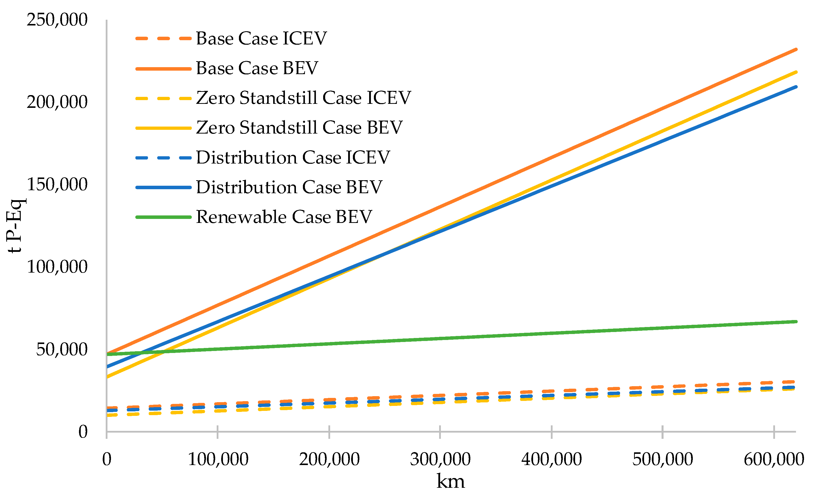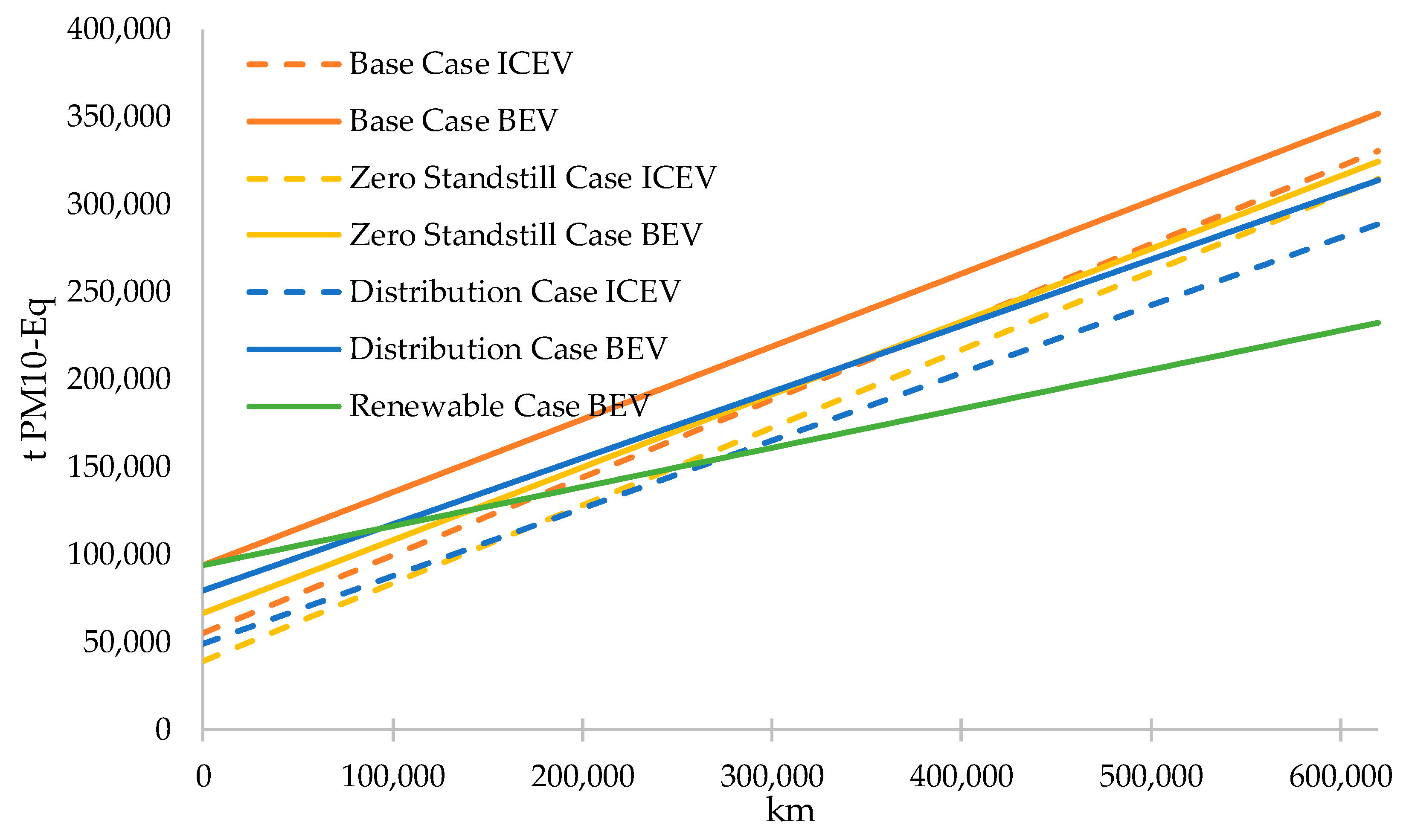[10]. This way, we obtain the vehicles’ average lifetime mileage: 206,396 km. We perform 100 additional calculations in which we scale the lifetime mileage between 0% to 300%. This results in an interval from 0 to 619,188 km. Only few vehicles might be able to reach a lifetime mileage of over 600,000 km. Nonetheless, this assumption enables the investigation of the influence of high lifetime mileages on vehicles’ LCA results.

Types of roads are urban and suburban roads as well as highways, which each differ in their respective free speeds, which are considered to calculate the respective consumption (

Table 1. Road categories.

Road Category	Free Speed (km/h)
Urban	v ≤ 50
Sub-urban	50 < v ≤ 100
Highway	v > 100

). The link-specific free speed is given by the simulation results (see Section 2.1.2).

We define three vehicle classes to account for the variability of different vehicle segments and simultaneously limit the level of detail (like in [43] and [6], see

Table 2. Vehicle classes.

Small	Medium	Large
Mini-Car	Compact Car	Mid-Range Car
Small Car	Mini-Van	Upper Mid-Range Car
	Large Capacity Van	Luxury Car
	Utilities	Sport Utility Vehicle
		Sports Car
		Off-Road Vehicle

). The classification of the German vehicle segments to the vehicle classes of small, medium and large corresponds to the investigations in [43]. We use the data sets from Ecoinvent version 3.6 for LCA [20].

Both ICEVs and BEVs consist of the same vehicle body (chassis, steering, suspension, brakes, tires, interior and drive-independent electronic components) for the respective vehicle class to maintain comparability (like in [10]). The corresponding Ecoinvent process “glider production, passenger car” is based on the inventory analysis of a Golf A4. According to Del Duce et al., the gasoline-fueled vehicle body has a share of 74% of the whole vehicle mass, diesel-fueled 69% and a BEV body without the battery has a share of 91% [44]. With the vehicle weights (from [43]) and the vehicle body and drive train shares, we calculate the mass for the respective vehicle size (

Table 3. Vehicle specifications.

Vehicle Body Share (%)			Vehicle Mass (kg)	Battery Capacity (kWh)	Battery Weight (kg)
battery electric	91 (w/o battery)	small	1199	25	333
		medium	1677	40	533
		large	2329	75	1000
gasoline-fueled	74	small	1068	-	-
		medium	1411	-	-
		large	1639	-	-
diesel-fueled	69	small	1137	-	-
		medium	1503	-	-
		large	1745	-	-

). The material composition of the vehicle classes mainly differs for the lightweight components [45]. Therefore, we adapt aluminum and steel shares. According to [10], the aluminum share of small vehicles is 20% lower than for medium-sized vehicles and for a large vehicle, it is 10% higher. We expect that the aluminum share of a medium-sized vehicle is 100% and change the values for small and large vehicles accordingly.

We adopt the respective Ecoinvent processes for the EoL of the vehicle bodies and drives. We adjust the material composition according to the production of the products. Some parts of aluminum, iron, copper, plastics and electric components are recyclable according to [44]. The materials for production consist of secondary material [10], the respective share is presented in

Table 4. Share of secondary materials.

Aluminum	Copper	Lead	Platinum
32%	44%	75%	5%

. We use the Ecoinvent cut-off system model for allocation [20]. This means, in short, that recyclable materials are burden free for recycling processes and that the recycling process is allocated to the recycled materials.

We use the Ecoinvent process “internal combustion engine production, passenger car” as a basis for the drive train of the ICEV and scale it according to the shares of the diesel- and gasoline-fueled drive trains. This process includes the engines, the gears, the tanks, the air conditioning and the exhaust systems. As stated in [10], the platinum and palladium contents in the ICEVs’ exhaust systems are considerably relevant in comparison to the BEV drive train. Helms et al. (2016) adjusted the contents according to the vehicle weights. Thus, we adapted the values for the respective vehicle classes and types (

Table 5. Platinum and palladium contents.

	Diesel			Gasoline
	Small	Medium	Large	Small	Medium	Large
Platinum (g)	2	4	7.5	0.5	0.5	0.5
Palladium (g)	0	0	0	1	2.5	5

).

The fuel consumption of the ICEVs is adopted from [46] and categorized by urban roads, suburban roads and highways (Table 1).

In Germany, fossil fuels contain biofuel components [10]. We assumed that diesel consists of 8.7% rape seed oil and that petrol consists of bioethanol from wheat with a 5% share. Those fuels are supplied on the markets for fuel supply in Europe, which are deposited in Ecoinvent.

For the BEV drive train, we apply the process “powertrain, for electric passenger car”. It includes the motor, the charger, the power electronics, the converter and the inverter [44]. We choose the battery capacities for the vehicle sizes small and medium according to [45]. These capacities correspond to current vehicle models in the respective segments [10]. We model the production of the battery with the Ecoinvent process “battery production, Li-ion, rechargeable, prismatic”. The data are provided by [47]. We add a transport per ship from Beijing to Amsterdam and transport per truck of 1000 km within Europe for the batteries. Most electric vehicles in the vehicle class large are luxury cars. Consequently, we adjust this vehicle class with the specification of a Tesla Model S. The basic version has a battery with a 75 kWh capacity [48]. The calculated vehicle mass is 100 kg heavier compared to the real vehicle, caused by the battery’s energy density and assuming the same vehicle bodies for all drive train types (Table 3). We adopt the electricity consumption from [45], for the vehicle classes small and medium (

Table 6. Vehicle- and road-Specific consumption.

		Urban Consumption	Suburban Consumption	Highway Consumption
Battery electric [kWh/100 km]	small	15	14	24
	medium	20	17	28
	large	25.9	25.2	37.8
Gasoline-fueled [l/100 km]	small	7.3	4.9	6.3
	medium	8.7	5.8	7.5
	large	10.5	7.2	9.2
Diesel-fueled [l/100 km]	small	5.7	3.8	4.5
	medium	6.7	4.5	5.3
	large	8.4	5.8	6.7

). These include charging losses. For the vehicle class large, we use the consumption values based on [48]. We assume a charging efficiency of 84% [49] to reflect charging losses (Table 6).

We use the German grid mix of the year 2018 to calculate the emissions of the BEV’s use phase. For this purpose, we adjust the Ecoinvent process “market for electricity, low voltage for Germany” (which in the current version v3.6 is based on the electricity mix of 2014) to the composition of gross electricity generation for 2018 estimated in [50]. The above process is composed of electricity production at medium and high voltage levels, the transformation to the low voltage level (relevant for charging), transmission losses and other emissions within the transformation. The construction of the power plant and electricity grid infrastructure is included in the process as well. We deduct electricity exports from the distribution of gross electricity generation to calculate the shares of the individual energy sources in the electricity available in Germany. As reported in [50], the exported electricity is based on the same electricity mix as the gross electricity generation. We include electricity imports, assuming the composition of the countries according to [51]. The resulting electricity mix for 2018 is shown in

Table 7. Shares grid mix Germany 2018 [51]

Lignite	20.95%	Nuclear Energy	10.95%	Others	3.81%
Wind	16.03%	Photovoltaics	6.67%	Water	3.65%
Hard Coal	11.90%	Biomass	6.51%	Waste	0.95%
Natural Gas	11.90%	Imports	5.88%	Oil	0.79%

.

All energy sources except waste and photovoltaics (PVs) are entered at the high-voltage level, waste at the medium-voltage level and PVs at the low-voltage level. If there are several processes for one energy source (e.g., onshore and offshore for wind energy), we modify the corresponding Ecoinvent processes with the respective shares.

We perform additional calculations, assuming a share of 100% renewable energies in the German grid mix. A 100% renewable grid mix in Germany for the year 2050 is presented in [52]. Accordingly, the adjusted grid mix contains of 30.4% PVs, 46.0% wind onshore and 23.6% wind offshore. This is an assumption for a theoretical renewable grid mix. For in-depth analysis of vehicles’ emissions in the year 2050, technological improvements have to be included. This is out of scope in this case study, but the here presented method enables the inclusion of future vehicle developments.

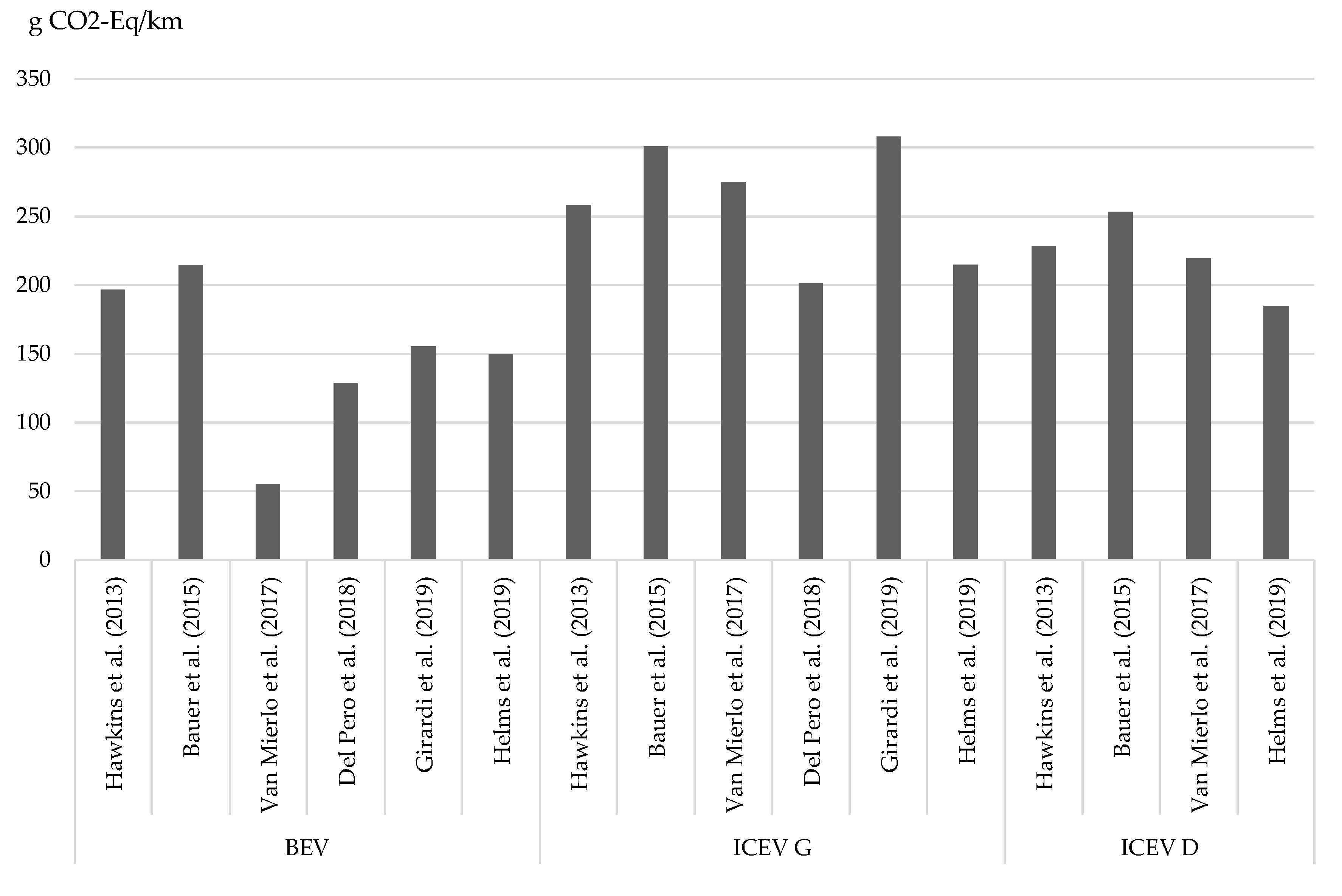
We perform an LCA for the generic vehicles, to compare the results with current research. Therefore, we apply the lifetime mileage and the road shares proposed by [10]: 168.000 km and 30% urban road, 40% suburban road and 30% highway. The road shares with the respective consumption result in the average consumption for the vehicles (

Table 8. Average consumption with respective road shares.

Diesel-Fueled (l/100 km)			Gasoline-Fueled (l/100 km)			Battery Electric (kWh/100 km)
Small	Medium	Large	Small	Medium	Large	Small	Medium	Large
6.04	7.18	8.79	4.58	5.4	6.85	17.3	21.2	29.19

). A broad spectrum of impact categories’ methods reduces the comparability. Therefore, we conduct studies which use similar methods (ReCiPe Midpoint). Nonetheless, this comparison is limited by different method versions (e.g., different year of publication).

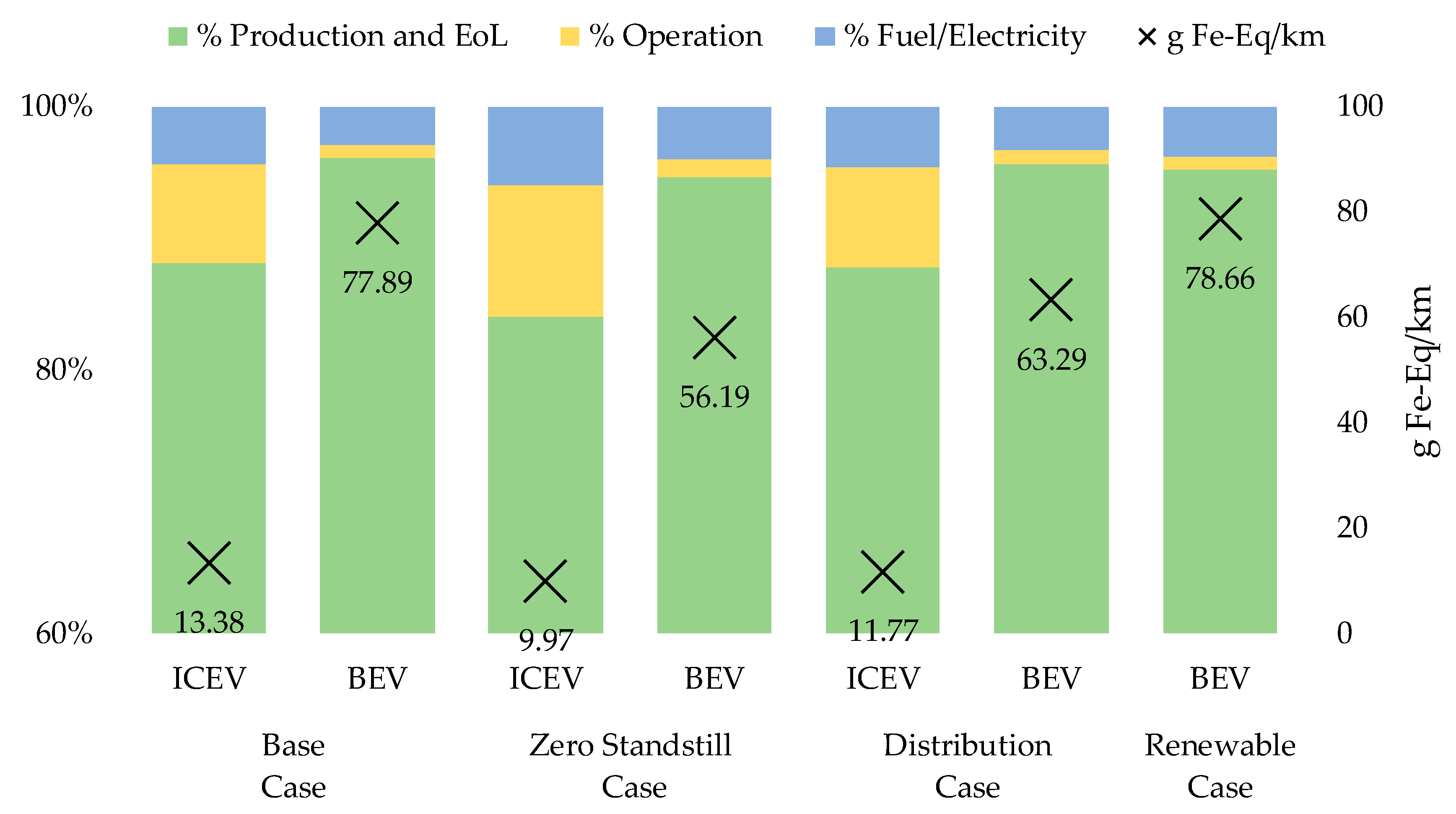
On an average day in Berlin or Brandenburg, 40% or 23% of the passenger cars are idle [53]. This results in a standstill of 29% for the region Berlin-Brandenburg, weighted according to the registered passenger cars (see Section 2.1.1). As these vehicles are not represented in the MATSim simulation, we assume 29% additional vehicles with zero covered distance. Moreover, we prepare the results without the additional vehicles to demonstrate the influence of standstill.

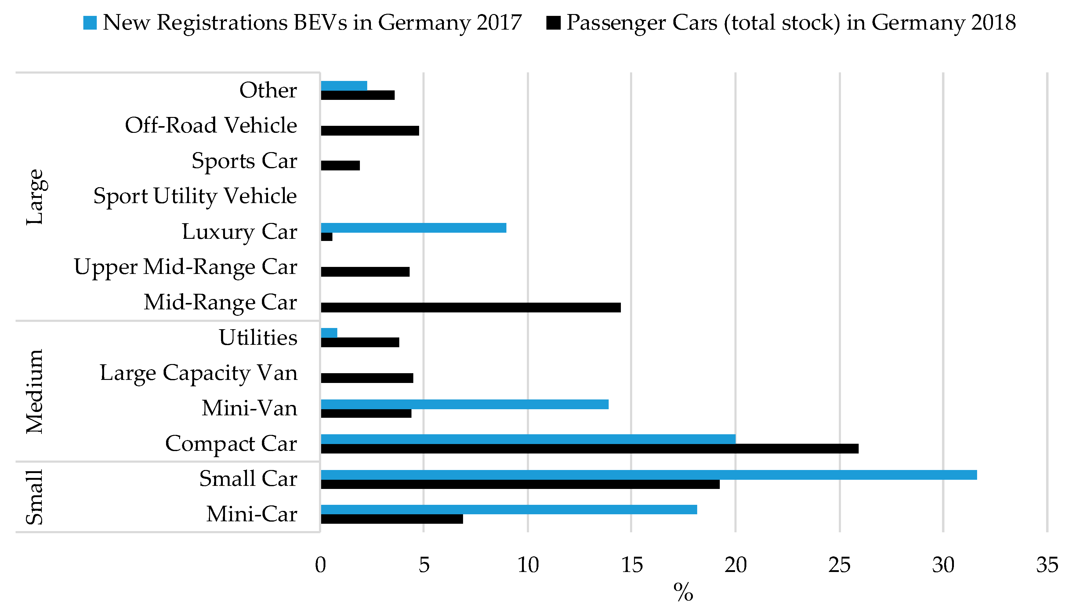
The MATSim simulation does (for now) not differentiate vehicle segments (e.g., mini-car) or size categories. Hence, the here defined vehicle classes must be assigned to the vehicles in the simulation. We convert the registered vehicles per vehicle segments (Figure 3 and Table 2) to the vehicle classes small, medium and large (

Table 9. Distribution vehicle classes.

Vehicle Class	Distribution Base Case	Distribution BEV 2017 Distribution Case
Small	27.10% (93.23% gasoline- and 7.77% diesel-fueled)	50.90%
Medium	40.10% (65.05% gasoline- and 34.98% diesel-fueled)	35.50%
Large	32.80% (49.30% gasoline- and 50.70% diesel-fueled)	13.60%

) and assign each vehicle in the MATSim simulation to one vehicle class and its respective attributes. For the ICEVs, we differentiate diesel- and gasoline-fueled vehicles. For further investigation of the vehicle distribution, we adjust the vehicle classes with the registration numbers of BEVs from 2017 (see Section 2.1.1, Table 9). We modify the BEV and ICEV distribution to display possible potentials of both technologies.

We modeled the direct emissions from the combustion (ICEV) based on the emissions from the corresponding processes (e.g., “transport, passenger car, medium size, diesel, EURO 5”) in Ecoinvent. The Ecoinvent data sets distinguish between consumption-dependent and -independent emissions. The independent emissions rest on the EURO 5 standard, but as the modeled vehicles in Ecoinvent are from 2010 and the consumption is based on a realistic drive cycle (EURO standards are based on driving cycles), the standards are exceeded [54]. Therefore, we parameterize the independent and dependent emissions according to the consumption of the ICEV and the emission factors for biofuels as defined by [55] (emission factors are −59 g CO₂-Eq./kWh for biodiesel and −52 g CO₂-Eq./kWh for bioethanol).

The abrasion of tires, brakes and roads is included using the Ecoinvent transport processes. The emissions are parameterized according to the vehicle weight. For the abrasion of BEV brakes, we assumed only 20% of the abrasion of ICEV brakes because of recuperation [44].

The maintenance of the vehicles is included in the Ecoinvent maintenance processes for the respective drive trains, parameterized for the lifetime mileage and the vehicle weight. The maintenance process for BEVs relies on the process for ICEVs. All ICEV-specific tasks (e.g., oil changes) are deleted (like in [44]). We discovered an unexplainable large amount of ethene as an output of the BEV process, which does not occur for the ICEV process. According to [44] (and additional E-mail correspondence with the authors), the amount of ethene should be equal for the maintenance of BEVs and ICEVs. Therefore, we adjusted the corresponding processes.

Additionally, the construction of road infrastructure and production facilities is included depending on the vehicle weight.

2.2.2. Impact Assessment

We perform the impact assessment using Ecoinvent data sets [20] and the included impact assessment methods. Like most studies, we include the GWP in our study, accompanied by the AP, EP, POFP, PMFP and metal depletion potential (MDP) (see

Table 10. Impact categories and methods.

Category	Name (Method (Version))	Unit
GWP	Climate change (ReCiPe Midpoint (Iv1.13))	kg CO2-Eq
AP	Terrestrial acidification (ReCiPe Midpoint (Iv1.13))	kg SO2-Eq
EP	Freshwater eutrophication (ReCiPe Midpoint (Iv1.13))	kg P-Eq
POFP	Photochemical oxidant formation (ReCiPe Midpoint (Iv1.13))	kg NMVOC-Eq
PMFP	Particulate matter formation (ReCiPe Midpoint (Iv1.13))	kg PM10-Eq
MDP	Metal depletion (ReCiPe Midpoint (Iv1.13))	kg Fe-Eq

GWP—Global Warming Potential; AP—Acidification Potential; EP—Eutrophication Potential; POFP—Photochemical Oxidation Potential; PMFP—Particulate Matter Formation Potential; MDP—Metal Depletion Potential; NMVOC—Non Methane Volatile Organic Compounds.

).

2.2.3. Implementation

We create three product systems for every vehicle type: vehicle production and EoL, vehicle operation and fuel or electricity consumption. It would also be possible to create one product system for all processes and calculate the impacts for each vehicle. However, as the program needs several minutes to calculate just one vehicle, this approach is inefficient for transport systems with a great number of vehicles. Therefore, we scale the results of the separated product systems depending on the covered distance, the vehicle weight and the fuel/electricity consumption for the whole life cycle within the program. This provides the vehicle results for the inventory analysis and the impact indicators differentiated according to the product systems: vehicle production and EoL depending on the vehicle weight in kg, vehicle operation depending on the covered distance in km and fuel or electricity consumption in kg or kWh. We included the battery size as an optional parameter, so it is adjustable. Simultaneously, the shares of the considered product systems in the respective impact categories are visible. Lastly, we sum up the vehicle results to get the results for the simulated MIT.

The LCA results need to be scaled to a 100% scenario, as the Open Berlin Scenario v5.3 represents only 10% of traffic flow (see Section 2.1.2). Therefore, we multiply the existing vehicles with their respective LCA results. The results of the 100% scenario are then related to the functional unit (total kilometers driven within the MIT). Additionally, we calculate the average lifetime mileage, consumption, road shares and vehicle weights.

2.2.4. Investigation Cases

For the MIT’s LCA, we perform four investigation cases: a base case in which we assume today’s German vehicle distribution, all standstill vehicles and Germany’s grid mix from 2018; a zero standstill case, in which vehicles that are not used are neglected; a distribution case, in which we assume the distribution of BEV registrations from 2017 for BEVs and ICEVs; and a renewable case, in which we assume a complete renewable grid mix for the use phase of BEVs. The reference year for all cases is 2018.

3. Results

This chapter displays the results on the vehicles’ LCA and the MIT’s LCA, using the vehicle LCA’s results. First, we validate the results of the vehicles’ LCA with the current literature. The second part of the results section covers the results for Berlin’s MIT investigation cases (see Section 2.2.4). The diagrams serve as an overview; detailed results are shown in the Supplementary Materials.

3.1. Validation Synthetic Vehicles

We assumed Germany’s grid mix from 2018 (see Section 2.2.1) and a lifetime mileage of 168,000 km. The results vary for the vehicle classes and types, and for the impact category (Figure 4, Figure 5, Figure 6, Figure 7, Figure 8, Figure 9 and Figure 10).

The electric vehicle has the lowest GWP for all vehicle classes except large, although it has the highest share in production and EoL compared to the diesel- and gasoline-fueled vehicles. Especially for the large electric vehicles, the battery causes marginally higher GWP, compared to the large diesel-fueled vehicle (Figure 4 and Figure 5).

The results for GWP are consistent with other studies [5,19]. Others present even lower GHG emissions for BEVs [3,26]. Helms et al. summarized the GWP of vehicles from different studies and described seven main influencing factors: lifetime mileage, energy consumption in use phase, grid mix, battery capacity, battery density, battery chemistry and GHG emissions from battery production [19]. The results of different studies vary widely due to a great variation in these factors (see Figure 1).

The gasoline-fueled vehicle shows the lowest AP for all vehicle classes, followed by the diesel-fueled car. The BEV has the highest impact regarding AP. Major contributors are the production, EoL (especially the battery production) and the electricity consumption (main contributors: electricity from hard coal, lignite and biomass) during driving (Figure 6). For the ICEV, the fuel consumption is the main source of sulfur dioxide equivalent emissions.

The results of the vehicles’ AP lie within the same range (0.92 to 0.94 g SO₂-Eq/km), like the results presented by [25] and [5]. Other studies, like [3] or [4], used different impact methods (CML2001 air acidification and acidification midpoint (mole of H+ eq.)). Therefore, a comparison of the total values is not recommended. Nonetheless, the results by Del Pero et al. show higher values for BEVs than for ICEVs, like the results presented here [3]. Only Girardi et al. show a lower impact by BEVs than ICEVs [4].

Additionally, for EP, the BEV has the highest impact for all vehicle classes. In comparison to the ICEV fuel consumption, the electricity consumption has a dominant share in BEV EP. Within the grid mix, the electricity produced with lignite causes high phosphor equivalent emissions (Figure 7).

For EP, the results show a sufficient compliance (deviation of around 15% to 25%) with the results presented by [25] and [5]. Other studies used different impact methods, therefore, we waive further comparisons.

The diesel-fueled vehicle has the greatest impact regarding POFP, with a major share of diesel consumption. The small diesel-fueled vehicle shows higher emissions than the medium and large BEV and gasoline-fueled vehicle. For the BEV, the production and EoL have a comparatively high share in POFP (Figure 8).

The results for the BEV for the POFP are reflected by the results presented in [3,4,5,25]. All show a comparable range (0.35 to 0.64 g NMVOC-Eq/km (NMVOC—Non-Methane Volatile Organic Compounds) for small- to medium-sized vehicles) for the respective results. Del Pero et al. and Bauer et al. computed the lowest NMVOC emissions for the gasoline-fueled vehicle [3,25] and Hawkins et al. and Girardi et al. for the BEV, but the latter did not assess any diesel-fueled vehicles [4,5].

For the small vehicle class, the diesel-fueled vehicles show the highest impact regarding PMFP, and around 40–50% of the emissions are caused by diesel consumption. In the medium class, the BEV passes the diesel-fueled vehicle slightly and, in the large class, the difference is substantial. The battery production of the EV is a major contributor to the PMFP. Abrasion by tires, brakes and roads contributes around 2% for ICEVs. For BEVs, the share is significantly smaller (Figure 9).

For PMFP, Hawkins et al., Girardi et al. and Bauer et al. presented values in the same range like the results presented here [4,5,25]. In [5] and [25], the ICEVs have fewer PM10 emissions than BEVs. In [4], the gasoline-fueled vehicle emits fewer PM10 emissions. Del Pero et al. used the following impact method: particulate matter/respiratory inorganics midpoint in kg PM2.5 eq. [3]. Therefore, we waive comparisons.

The BEV has the highest values for MDP. For all vehicles, the production and EoL are the major contributors to MDP. The fuel and electricity consumption as well as the operation (including, e.g., maintenance) have less than a 10% share in MDP (Figure 10).

The results for MDP have the same ratio as in [5]. There is a great lack of knowledge on metal depletion and other resource use-related potentials (see [18]).

3.2. Case Study: Results for Berlin’s Motorized Individual Transport

The GWP for the ICEV and BEV base case is between the values for small- and medium-sized vehicles (see Figure 4 and Figure 11). The BEV base case emits around 20% less CO₂-Eq. emissions per kilometer than the ICEV base case. The zero standstill case (we assume 29% standstill for the base case, see Section 2.2.1.) results in smaller values. The share of production and EoL decreases for both the ICEV and BEV zero standstill cases. The difference for the ICEV zero standstill case is 5.60% and for the BEV zero standstill case is 9.70% compared to the respective base case. The gap between the base case and the distribution case (we assume the vehicle distribution from the new registrations of BEVs in 2017 for BEVs and ICEVs, while the shares of gasoline-powered vs. diesel-powered vehicles remain the same, see Section 2.1.1) is slightly higher: 7.38% less GHG emissions for the ICEV distribution case and 10.08% for the BEV distribution case compared to the respective base case. However, the share of production and EoL decreases. The only renewable energy case (only renewable energies, see Section 2.2.1.) shows more substantial differences: the kilometer-specific GHG emissions are 52.76% smaller than in the base case (regarding BEVs) and the share of production and EoL increases significantly.

The investigation of the lifetime mileage (see Section 2.2.1) shows that the breakeven point for the GWP is at about 55,000 km for the base cases (Figure 12). With a higher lifetime mileage, a BEV MIT emits less GHG emissions than the ICEV MIT. The ICEV base case has lower GHG emissions for production (see Figure 12 at lifetime mileage = 0) for production and EoL but deteriorates with increasing lifetime mileage.

The results for the AP show higher values for the BEV base case than for the ICEV base case (Figure 13). These values decrease for all cases. A substantial decrease is visible for the BEV renewable case: the sulfur dioxide equivalents reduce by 44.76%. Simultaneously, the share of production and EoL rises over 75%. For the AP, the ICEV base case starts with a burden half as high as the BEV base case. The gap stays nearly constant for rising lifetime mileage (Figure 14). BEVs reach lower values only for the renewable case (Figure 14).

The base case reveals a noticeable advantage of ICEVs regarding phosphor equivalent emissions (Figure 15), comparable with the synthetic vehicles results. Even the renewable case accounts for more than 250% of the ICEV base case emissions (Figure 16).

For POFP, the BEV base case generates smaller values compared to the ICEV base case. This advantage increases with the use of renewable energies (Figure 17). Although the values for production and EoL are higher for BEVs, after 30,000 to 100,000 km (depending on the respective case) the investigation cases reach the breakeven points (Figure 18).

For PMFP, ICEVs have lower emissions compared to BEVs. Only the BEV renewable case shows lower emissions than the ICEV base case (Figure 19). As the BEV production and EoL values are noticeably higher, the BEV cases only demonstrate lower values for high lifetime mileage (Figure 20).

For MDP, the advantages of the ICEV cases are tremendous (Figure 21). Production has a share of over 80% for all cases. Subsequently, the BEV renewable case shows only slight differences. However, the zero standstill and distribution cases demonstrate higher gains in comparison to the base cases (BEVs and ICEVs). In addition, the consideration of MDP over lifetime mileage shows only slight gains. In contrast to all other investigated impact categories, covering the energy demand with renewable sources even increases the MDP (Figure 22).

4. Discussion

The BEV base case shows advantages for the GWP and POFP compared to the ICEV base case. With renewable energy as an electricity source, it gains additional advantages regarding the AP and comparable results to the ICEV base case regarding the PMFP. The ICEV base case has smaller emissions regarding the EP and MDP for all cases. The zero standstill case results in smaller values for all impact categories compared to the base case for both MIT systems. This is a logical consequence of assuming 0% standstill and therefore fewer vehicles with no mileage, especially for the production- and EoL-intensive categories like MDP. There are only slight differences for the fuel- or electricity-dependent categories (e.g., GWP, AP and POFP). The zero standstill case implies inspiration for mobility on demand (MOD) or car sharing services, like Ding et al. investigated [16]. A reduction of the total number of vehicles which are used to cover the same ways leads to smaller life cycle emissions. Advantages are conceivable, even with an increase in mileage for the MIT. The here developed method allows us to investigate possible effects of MOD or even autonomous MOD services with vehicle concepts introduced in [31]. The distribution case demonstrates the advantages of a vehicle distribution consisting of a large share of small vehicles. The ICEV distribution case improves in all categories compared to the base case, slightly more in categories with high fuel dependence. On the contrary, the BEV distribution case shows similar improvements for production-intensive categories because of the battery sizes of the respective vehicle classes. The renewable case considers renewable energies only for the driving consumption and even gains advantages in all investigated impact categories. Helmers et al. imply major advantages from battery cell production with renewable energies [23]. Additionally, the results by Almeida et al. demonstrate great savings of greenhouse gas emissions for newer Li-ion batteries compared to older ones [11].

Jaeger et al. underline the spatial and temporal dependence of air pollutants [17]. This study represents POFP and PMFP for the whole life cycle, including production and EoL (which often do not happen at the place of use). The results imply a slight advantage of the BEV base case in PMFP considering only the use phase. However, this still includes the emissions that are not emitted and effective locally. Moreover, the Open Berlin Scenario covers, among others, suburban and rural roads, which often do not suffer from air pollution. The first approaches emphasize the combination of a detailed air pollutant investigation in the use phase with the road network from the Open Berlin Scenario.

Dér et al. point out that the ambient temperature has a remarkable effect on the energy consumption of BEVs [12]. Their field test has shown that cooling and heating systems account for an increase of 24 or 38% in energy demand in summer and winter conditions. The here presented consumption values are averages for the respective vehicle classes and drive trains.

We assign the vehicle distribution randomly to the vehicles of the Open Berlin Scenario. This results in a similar resolution for the lifetime mileage of the respective vehicles. Caused by the standstill restriction, the share of vehicles with a modest lifetime mileage is higher than in [53]. Additionally, we compare the shares of the vehicle classes’ lifetime mileage, resulting in noticeable differences. Nonetheless, the referenced study displays a picture of Germany. However, Berlin-Brandenburg is an urban region with different conditions. We provide the distribution case to show the potential of different vehicle distributions.

The data provided by Ecoinvent were collected several years ago. We adjust certain parameters and the results of the synthetic vehicles are comparable to current studies. Still, further changes with the latest date are pending. According to Notter et al., cathode material production has the greatest influence on the ecological impacts of vehicle batteries [47]. Simultaneously, Helms et al. reported that the results for the production of different cathode materials vary more than 20% depending on the chosen impact category [10]. However, Notter et al. argues that the difference varies less than 2% regarding a vehicle cradle-to-gate [47].

The results display midpoint results of the conducted ReCiPe methods. This prohibits assertion on the environmental impact as a whole. However, impacts in the respective impact categories are displayed.

In contrast to the use of statistical data, the here presented method enables the analysis of other versions of the Open Berlin Scenario (e.g., with changing operation strategies). Extensions to other transport sectors, like waste collection (presented in [56]) or freight traffic (presented in [36]), are possible with the respective vehicle data. The usage of other databases and/or traffic simulations is possible with a certain effort.

The study investigated environmental impacts of battery electric passenger cars, which solely replace ICEVs. Nonetheless, investigations on areas like vehicle ownership, autonomous vehicles and others are possible with the respective transport simulations.

5. Conclusions

We presented a method that combines agent-based transport simulation and LCAs. Therefore, we provided a literature review on the latest LCA studies and introduced the case study (Berlin’s motorized transport sector). We developed synthetic vehicles and compared their impacts to current research. Furthermore, we established approaches to investigate the influence of lifetime mileage, vehicle distribution, energy supply and standstill. Sole vehicle LCAs enable the comparison of the conducted vehicles, but neglect influences and opportunities of whole transport systems. The developed method facilitates the analysis of environmental effects of new technologies and strategies in transportation. We showed the influence of different vehicle distributions and a reduction of vehicles, but further analyses (e.g., city-wide autonomous driving) are possible. The BEV base case has smaller impacts regarding the GWP and POFP compared to the ICEV base case. This implies that today’s MIT gains advantages regarding climate change if operating with electric vehicles. In the renewable case, it gains additional advantages regarding the AP and similar results to the ICEV base case regarding the PMFP. Additionally, GHG emissions are reduced by over 60%. ICEVs have smaller emissions regarding the EP and MDP for all cases. The zero standstill case and distribution case demonstrate reduced emissions in all categories. The zero standstill case allows us to imagine mobility on-demand services: the total number of vehicles is reduced as multiple users have access to the vehicles. Especially for BEVs (with high production emissions), the zero standstill case shows fewer emissions than the base case. For ICEVs, the gap is much smaller. Nonetheless, influences of real mobility on-demand scenarios (e.g., additional routes and therefore an increased number of driven kilometers) need further research. The distribution case exhibits the benefits of a shift to smaller vehicles. The new distribution reduced the GHG emissions for BEVs by 10.1% and for ICEVs by 7.4%. The use of BEVs with renewable energies, accompanied by a vehicle distribution consisting of mostly small vehicles and mobility on-demand services, provides a chance to achieve the German climate goals for transport in the future.

Future approaches will focus on different levels: time-dependent LCA data for vehicles and batteries to develop a vehicle segment and time-dependent vehicle distribution; the implementation of further transport simulation results to investigate other transport sectors, like freight or waste collection, and strategy options like mobility on-demand or autonomous driving; the comparison to other technologies like fuel-cell vehicles; the deployment of endpoint results to enable assertions on the ecological impact; a detailed consumption model including ambient temperatures that allows for local and temporal investigations of air pollutant emissions and displays the use phase emissions in more detail.

References

1. DIN e. V. (Hrsg.). DIN EN ISO 14040: Umweltmanagement—Ökobilanz—Grundsätze und Rahmenbedingungen (ISO 14040:2006); Deutsche und Englische Fassung EN ISO 14040:2006; Beuth-Verlag: Berlin, Germany, 2009. [Google Scholar]
2. Burchart-Korol, D.; Folęga, P. Comparative Life Cycle Impact Assessment of Chosen Passenger Cars with Internal Combustion Engines. Transp. Probl. 2019, 14, 69–76. [Google Scholar] [CrossRef] [Green Version]
3. Del Pero, F.; Delogu, M.; Pierini, M. Life Cycle Assessment in the automotive sector: A comparative case study of Internal Combustion Engine (ICE) and electric car. Procedia Struct. Integr. 2018, 12, 521–537. [Google Scholar] [CrossRef]
4. Girardi, P.; Gargiulo, A.; Brambilla, P.C. A comparative LCA of an electric vehicle and an internal combustion engine vehicle using the appropriate power mix: The Italian case study. Int. J. Life Cycle Assess. 2015, 20, 1127–1142. [Google Scholar] [CrossRef]
5. Hawkins, T.R.; Singh, B.; Majeau-Bettez, G.; Strømman, A.H. Comparative Environmental Life Cycle Assessment of Conventional and Electric Vehicles. J. Ind. Ecol. 2013, 17, 53–64. [Google Scholar] [CrossRef]
6. Messagie, M.; Boureima, F.-S.; Coosemans, T.; Macharis, C.; Mierlo, J. A Range-Based Vehicle Life Cycle Assessment Incorporating Variability in the Environmental Assessment of Different Vehicle Technologies and Fuels. Energies 2014, 7, 1467–1482. [Google Scholar] [CrossRef]
7. Kawamoto, R.; Mochizuki, H.; Moriguchi, Y.; Nakano, T.; Motohashi, M.; Sakai, Y.; Inaba, A. Estimation of CO2 Emissions of Internal Combustion Engine Vehicle and Battery Electric Vehicle Using LCA. Sustainability 2019, 11, 2690. [Google Scholar] [CrossRef] [Green Version]
8. Dai, Q.; Kelly, J.C.; Gaines, L.; Wang, M. Life Cycle Analysis of Lithium-Ion Batteries for Automotive Applications. Batteries 2019, 5, 48. [Google Scholar] [CrossRef] [Green Version]
9. Peters, J.F.; Baumann, M.; Zimmermann, B.; Braun, J.; Weil, M. The environmental impact of Li-Ion batteries and the role of key parameters—A review. Renew Sustain. Energy Rev. 2017, 67, 491–506. [Google Scholar] [CrossRef]
10. Helms, H.; Jöhrens, J.; Kämper, C.; Giegrich, J.; Liebich, A.; Vogt, R.; Lambrecht, U. Weiterentwicklung und Vertiefte Analyse der Umweltbilanz von Elektrofahrzeugen. Available online: https://www.umweltbundesamt.de/publikationen/weiterentwicklung-vertiefte-analyse-der (accessed on 27 April 2020).
11. Almeida, A.; Sousa, N.; Coutinho-Rodrigues, J. Quest for Sustainability: Life-Cycle Emissions Assessment of Electric Vehicles Considering Newer Li-Ion Batteries. Sustainability 2019, 11, 2366. [Google Scholar] [CrossRef] [Green Version]
12. Dér, A.; Erkisi-Arici, S.; Stachura, M.; Cerdas, F.; Böhme, S.; Herrmann, C. Life Cycle Assessment of Electric Vehicles in Fleet Applications. In Fleets Go Green; Herrmann, C., Mennenga, M.S., Böhme, S., Eds.; Springer: Berlin/Heidelberg, Germany, 2018; pp. 61–80. [Google Scholar]
13. de Souza, L.L.P.; Lora, E.E.S.; Palacio, J.C.E.; Rocha, M.H.; Renó, M.L.G.; Venturini, O.J. Comparative environmental life cycle assessment of conventional vehicles with different fuel options, plug-in hybrid and electric vehicles for a sustainable transportation system in Brazil. J. Clean. Prod. 2018, 203, 444–468. [Google Scholar] [CrossRef]
14. Lajunen, A.; Kivekäs, K.; Vepsäläinen, J.; Tammi, K. Influence of Increasing Electrification of Passenger Vehicle Fleet on Carbon Dioxide Emissions in Finland. Sustainability 2020, 12, 5032. [Google Scholar] [CrossRef]
15. Torzynski, S.; Göhlich, D.; Hahn, D.; Bryl-Radziemska, M. E-Bus Berlin—Betrieb der Buslinie 204 (Vormals: Buslinie 147) Mit Einer Flotte von Elektrobussen Inklusive Infrastruktur zur Induktiven Zwischenladung: FuE-Programm “Schaufenster Elektromobilität” der Bundesregierung: Gemeinsamer Abschlussbericht: Internationales Schaufenster Elektromobilität Berlin-Brandenburg: Laufzeit des Vorhabens vom: 01.01.2013 bis: 30.09.2016: Abschlussbericht. Available online: https://www.tib.eu/de/suchen/id/TIBKAT:880375914/ (accessed on 21 July 2020).
16. Ding, N.; Pan, J.; Zhang, Z.; Yang, J. Life cycle assessment of car sharing models and the effect on GWP of urban transportation: A case study of Beijing. Sci. Total Environ. 2019, 688, 1137–1144. [Google Scholar] [CrossRef] [PubMed]
17. Jaeger, F.A.; Müller, K.; Petermann, C.; Lesage, E. LCA in Strategic Decision Making for Long Term Urban Transportation System Transformation. In Designing Sustainable Technologies, Products and Policies: From Science to Innovation; Benetto, E., Gericke, K., Guiton, M., Eds.; Springer: Berlin/Heidelberg, Germany, 2018; pp. 193–204. [Google Scholar]
18. Dolganova, I.; Rödl, A.; Bach, V.; Kaltschmitt, M.; Finkbeiner, M. A Review of Life Cycle Assessment Studies of Electric Vehicles with a Focus on Resource Use. Resources 2020, 9, 32. [Google Scholar] [CrossRef] [Green Version]
19. Helms, H.; Kämper, C.; Biemann, K.; Lambrecht, U.; Jöhrens, J.; Meyer, K. Klimabilanz von Elektroautos: Einflussfaktoren und Verbesserungspotenzial. Available online: https://www.agora-verkehrswende.de/veroeffentlichungen/klimabilanz-von-elektroautos/ (accessed on 21 July 2020).
20. Wernet, G.; Bauer, C.; Steubing, B.; Reinhard, J.; Moreno-Ruiz, E.; Weidema, B. The ecoinvent database version 3 (part I): Overview and methodology. Int. J. Life Cycle Assess. 2016, 21, 1218–1230. [Google Scholar] [CrossRef]
21. GaBi LCA Database Documentation. Available online: https://www.gabi-software.com/support/gabi (accessed on 7 May 2020).
22. Tagliaferri, C.; Evangelisti, S.; Acconcia, F.; Domenech, T.; Ekins, P.; Barletta, D.; Lettieri, P. Life cycle assessment of future electric and hybrid vehicles: A cradle-to-grave systems engineering approach. Chem. Eng. Res. Des. 2016, 112, 298–309. [Google Scholar] [CrossRef]
23. Helmers, E.; Dietz, J.; Weiss, M. Sensitivity Analysis in the Life-Cycle Assessment of Electric vs. Combustion Engine Cars under Approximate Real-World Conditions. Sustainability 2020, 12, 1241. [Google Scholar] [CrossRef] [Green Version]
24. Skrúcaný, T.; Kendra, M.; Stopka, O.; Milojević, S.; Figlus, T.; Csiszár, C. Impact of the Electric Mobility Implementation on the Greenhouse Gases Production in Central European Countries. Sustainability 2019, 11, 4948. [Google Scholar] [CrossRef] [Green Version]
25. Bauer, C.; Hofer, J.; Althaus, H.-J.; Del Duce, A.; Simons, A. The environmental performance of current and future passenger vehicles: Life cycle assessment based on a novel scenario analysis framework. Appl. Energy 2015, 157, 871–883. [Google Scholar] [CrossRef]
26. van Mierlo, J.; Messagie, M.; Rangaraju, S. Comparative environmental assessment of alternative fueled vehicles using a life cycle assessment. Transp. Res. Procedia 2017, 25, 3435–3445. [Google Scholar] [CrossRef]
27. Berger, M.; Sonderegger, T.; Alvarenga, R.; Bach, V.; Cimprich, A.; Dewulf, J.; Frischknecht, R.; Guinée, J.; Helbig, C.; Huppertz, T.; et al. Mineral resources in life cycle impact assessment: Part II—Recommendations on application-dependent use of existing methods and on future method development needs. Int. J. Life Cycle Assess. 2020, 25, 798–813. [Google Scholar] [CrossRef] [Green Version]
28. Sonderegger, T.; Berger, M.; Alvarenga, R.; Bach, V.; Cimprich, A.; Dewulf, J.; Frischknecht, R.; Guinée, J.; Helbig, C.; Huppertz, T.; et al. Mineral resources in life cycle impact assessment—Part I: A critical review of existing methods. Int. J. Life Cycle Assess. 2020, 25, 784–797. [Google Scholar] [CrossRef]
29. Jahn, R.M.; Syré, A.; Grahle, A.; Schlenther, T.; Göhlich, D. Methodology for Determining Charging Strategies for Urban Private Vehicles based on Traffic Simulation Results. Procedia Comput. Sci. 2020, 170, 751–756. [Google Scholar] [CrossRef]
30. Gong, H.; Zou, Y.; Yang, Q.; Fan, J.; Sun, F.; Goehlich, D. Generation of a driving cycle for battery electric vehicles: A case study of Beijing. Energy 2018, 150, 901–912. [Google Scholar] [CrossRef]
31. Grahle, A.; Song, Y.-W.; Brüske, K.; Bender, B.; Göhlich, D. Autonomous Shuttles for Urban Mobility on Demand Applications—Ecosystem Dependent Requirement Elicitation. Proc. Des. Soc. Des. Conf. 2020, 1, 887–896. [Google Scholar] [CrossRef]
32. Kohl, J.L.; van der Schoor, M.J.; Syré, A.M.; Göhlich, D. Social Sustainability in the Development of Service Robots. Proc. Des. Soc. Des. Conf. 2020, 1, 1949–1958. [Google Scholar] [CrossRef]
33. Onat, N.; Kucukvar, M.; Tatari, O. Towards Life Cycle Sustainability Assessment of Alternative Passenger Vehicles. Sustainability 2014, 6, 9305–9342. [Google Scholar] [CrossRef] [Green Version]
34. Horni, A.; Nagel, K.; Axhausen, K.W. The Multi-Agent Transport Simulation MATSim. Available online: http://ci.matsim.org:8080/job/MATSim-Book/ws/partOne-latest.pdf (accessed on 17 August 2020).
35. Ziemke, D.; Kaddoura, I.; Nagel, K. The MATSim Open Berlin Scenario: A multimodal agent-based transport simulation scenario based on synthetic demand modeling and open data. Procedia Comput. Sci. 2019, 151, 870–877. [Google Scholar] [CrossRef]
36. Martins-Turner, K.; Grahle, A.; Nagel, K.; Göhlich, D. Electrification of Urban Freight Transport—A Case Study of the Food Retailing Industry. Procedia Comput. Sci. 2020, 170, 757–763. [Google Scholar] [CrossRef]
37. Senatsverwaltung für Umwelt, Verkehr und Klimaschutz. Mobilität der Stadt: Berliner Verkehr in Zahlen. Available online: https://www.berlin.de/sen/uvk/verkehr/verkehrsdaten/zahlen-und-fakten/mobilitaet-der-stadt-berliner-verkehr-in-zahlen-2017/ (accessed on 21 July 2020).
38. Kraftfahrt Bundesamt. Bestand an Kraftfahrzeugen und Kraftfahrzeuganhängern nach Zulassungsbezirken, 1. January 2019. Available online: https://www.kba.de/DE/Statistik/Produktkatalog/produkte/Fahrzeuge/fz1_b_uebersicht.html (accessed on 23 April 2020).
39. Kraftfahrt Bundesamt. Bestand an Personenkraftwagen nach Segmenten und Modellreihen am 1. January 2019. Available online: https://www.kba.de/DE/Statistik/Produktkatalog/produkte/Fahrzeuge/fz12_b_uebersicht.html (accessed on 23 April 2020).
40. Kraftfahrt Bundesamt. Neuzulassungen im Jahr 2017 nach Umwelt-Merkmalen. Available online: https://www.kba.de/DE/Statistik/Produktkatalog/produkte/Fahrzeuge/fz14_n_uebersicht.html (accessed on 23 April 2020).
41. OpenStreetMap. Available online: https://www.openstreetmap.org (accessed on 23 April 2020).
42. Bäumer, M.; Hautzinger, H.; Pfeiffer, M.; Stock, W. Fahrleistungserhebung 2014: Infandsfahrleistung und Unfallrisiko. Available online: https://www.bmvi.de/SharedDocs/DE/Artikel/G/fahrleistungserhebung.html (accessed on 23 April 2020).
43. Hülsmann, F.; Mottschall, M.; Hacker, F.; Kasten, P. Konventionelle und Alternative Fahrzeugtechnologien bei PKW und Schweren Nutzfahrzeugen: Potenziale zur Minderung des Energieverbrauchs bis 2050. Available online: https://www.google.com/url?sa=t&rct=j&q=&esrc=s&source=web&cd=1&ved=2ahUKEwjB14DywP_oAhWCy6QKHW9gBecQFjAAegQIAhAB&url=https%3A%2F%2Fwww.oeko.de%2Foekodoc%2F2105%2F2014-662-de.pdf&usg=AOvVaw1tg7-SHn5JGu4JRlZJU27q (accessed on 23 April 2020).
44. Del Duce, A.; Gauch, M.; Althaus, H.-J. Electric passenger car transport and passenger car life cycle inventories in ecoinvent version 3. Int. J. Life Cycle Assess. 2016, 21, 1314–1326. [Google Scholar] [CrossRef]
45. Öko-Institut; DLR-Institut für Verkehrsforschung. Renewbility: Stoffstromanalyse Nachhaltige Mobilität im Kontext Erneuerbarer Energien bis 2030. Available online: https://www.oeko.de/publikationen/p-details/renewbility-stoffstromanalyse-nachhaltige-mobilitaet-im-kontext-erneuerbarer-energien-bis-2030 (accessed on 21 July 2020).
46. Knörr, W.; Heidt, C.; Goers, S.; Bergk, F. Aktualisierung Daten-und Rechenmodell: Ener-Gieverbrauch und Schadstoffemissionen des Mo-Torisierten Verkehrs in Deutschland 1960–2035 (TREMOD) für Die Emissionsberichterstattung 2016 (Berichtsperiode 1990–2014). Available online: https://www.ifeu.de/methoden/modelle/tremod/ (accessed on 22 April 2020).
47. Notter, D.A.; Gauch, M.; Widmer, R.; Wäger, P.; Stamp, A.; Zah, R.; Althaus, H.-J. Contribution of Li-Ion Batteries to the Environmental Impact of Electric Vehicles. Environ. Sci. Technol. 2010, 44, 6550–6556. [Google Scholar] [CrossRef]
48. ADAC e. V. Tesla Model S Performance. Available online: https://www.adac.de/_ext/itr/tests/Autotest/AT5022_Tesla_Model_S_Performance/Tesla_Model_S_Performance.pdf (accessed on 24 April 2020).
49. ADAC e. V. Aktuelle Elektroautos im Test: So hoch ist der Stromverbrauch. Available online: https://www.adac.de/rund-ums-fahrzeug/tests/elektromobilitaet/stromverbrauch-elektroautos-adac-test/ (accessed on 24 April 2020).
50. Icha, P.; Kuhs, G. Entwicklung der Spezifischen Kohlendioxid- Emissionen des Deutschen Strommix in den Jahren 1990–2018. Available online: https://www.umweltbundesamt.de/publikationen/entwicklung-der-spezifischen-kohlendioxid-5 (accessed on 20 April 2020).
51. AG Energiebilanzen e. V. Auswertungstabellen zur Energiebilanz Deutschland: Daten für die Jahre 1990 bis 2018. Stand: März 2020 (Endgültige Ergebnisse bis 2018). Available online: https://ag-energiebilanzen.de/#awt_2018_d (accessed on 20 April 2020).
52. Henning, H.-M.; Palzer, A. Energiesystem Deutschland 2050. Available online: https://www.ise.fraunhofer.de/de/veroeffentlichungen/studien/studie-energiesystem-deutschland-2050.html (accessed on 20 April 2020).
53. infas, DLR, IVT and infas 360. Mobilität in Tabellen (MiT 2017): Mobilität in Deutschland. Available online: https://www.mobilitaet-in-tabellen.de/mit/ (accessed on 21 July 2020).
54. Simons, A. Road transport: New life cycle inventories for fossil-fuelled passenger cars and non-exhaust emissions in ecoinvent v3. Int. J. Life Cycle Assess. 2016, 21, 1299–1313. [Google Scholar] [CrossRef]
55. Lauf, T.; Memmler, M.; Schneider, S. Emissionsbilanz Erneuerbarer Energieträger: Bestimmung der Vermiedenen Emissionen im Jahr 2018. Available online: https://www.umweltbundesamt.de/publikationen/emissionsbilanz-erneuerbarer-energietraeger (accessed on 20 April 2020).
56. Ewert, R.; Grahle, A.; Martins-Turner, K.; Syré, A.; Nagel, K.; Göhlich, D. Electrification of Urban. Waste Collection: Introducing a Simulation-Based Methodology for Feasibility, Impact and Cost Analysis. VSP Work. Pap. 2020. Preprint. [Google Scholar] [CrossRef]
Figure 1. Global warming potential from several studies; BEV—battery electric vehicle, ICEV G—internal combustion engine vehicle gasoline, ICEV D—internal combustion engine vehicle diesel [3,4,5,19,25,26].
Sustainability 12 07302 g001
Figure 2. Flow chart method and use case.
Sustainability 12 07302 g002
Figure 3. Vehicle distributions in Germany by percentage [38,39,40].
Sustainability 12 07302 g003
Figure 4. Global warming potential—synthetic vehicles at 168,000 km lifetime mileage.
Sustainability 12 07302 g004
Figure 5. Global warming potential—vehicles over lifetime mileage.
Sustainability 12 07302 g005
Figure 6. Acidification potential—synthetic vehicles at 168,000 km lifetime mileage.
Sustainability 12 07302 g006
Figure 7. Eutrophication potential—synthetic vehicles at 168,000 km lifetime mileage.
Sustainability 12 07302 g007
Figure 8. Photochemical oxidant formation potential—synthetic vehicles at 168,000 km lifetime mileage.
Sustainability 12 07302 g008
Figure 9. Particulate matter formation potential—synthetic vehicles at 168,000 km lifetime mileage.
Sustainability 12 07302 g009
Figure 10. Metal depletion potential—synthetic vehicles at 168,000 km lifetime mileage.
Sustainability 12 07302 g010
Figure 11. Global warming potential—Motorized Individual Transport (MIT).
Sustainability 12 07302 g011
Figure 12. Global warming potential—MIT vs. lifetime mileage.
Sustainability 12 07302 g012
Figure 13. Acidification potential—MIT.
Sustainability 12 07302 g013
Figure 14. Acidification potential—MIT vs. lifetime mileage.
Sustainability 12 07302 g014
Figure 15. Eutrophication potential—MIT.
Sustainability 12 07302 g015
Figure 16. Eutrophication potential—MIT vs. lifetime mileage.
Sustainability 12 07302 g016
Figure 17. Photochemical oxidant formation potential—MIT.
Sustainability 12 07302 g017
Figure 18. Photochemical oxidant formation potential—MIT vs. lifetime mileage.
Sustainability 12 07302 g018
Figure 19. Particulate matter formation potential—MIT.
Sustainability 12 07302 g019
Figure 20. Particulate matter formation potential—MIT vs. lifetime mileage.
Sustainability 12 07302 g020
Figure 21. Metal depletion potential—MIT.
Sustainability 12 07302 g021
Figure 22. Metal depletion potential—MIT vs. lifetime mileage.
Sustainability 12 07302 g022