Approach to the Proecological Distribution of the Traffic Flow on the Transport Network from the Point of View of Carbon Dioxide

Abstract

Nowadays, apart from travel time and cost, more and more attention is paid to ensuring that ecological footprint of the means of transport used for a journey is as small as possible. Therefore, it is reasonable to look for methods and solutions that will allow planning communication connections according to the principles of sustainable development. The aim of the article was to present mathematical model of the proecological distribution of traffic flow into a network, together with a determination of how the amount of emissions of harmful compounds for rail transport will be calculated (based on amount of energy necessary for movement, calculated on circumference of the wheels). The model has been verified on real data. The traffic flow was distributed over a selected communication route: Warszawa—Gdansk, where the criterion was minimization of total carbon dioxide emissions. An evolutionary method implemented in Microsoft Excel was used to solve the optimization problem. For the analysis of only the fastest connections, the railway one was the optimal from the point of view of the adopted criteria. After the train capacity was exceeded, air and car connections were loaded. Based on the research, a function that represents the amount of carbon dioxide emissions in the analyzed traffic route depending on the size of the traffic flow was developed.

1. Introduction

Nowadays, apart from the travel time and cost, more and more attention is paid to ensuring that the ecological footprint of the means of transport used for the journey is as small as possible. Therefore, it is reasonable to look for methods and solutions that will allow planning communication connections according to the principle of sustainable development.

The subject of the article concerns the distribution of traffic flow on the network. In the literature, we can find many references to considerations in this direction. Usually, works present the theories relating to the traffic flow, with descriptions of various types of formalism used in the formulation of the problem, the optimization methods used, or using optimization and simulation tools. The multitude of publications proves that the subject is popular and still relevant. One of the tools that allows for appropriate “control” of the traffic flow, which will ensure a sufficiently low negative impact of passenger movement on the environment, is to distribute the traffic flow over the network and on this basis adaptation of the transport offered accordingly. Therefore, this article is devoted to this subject. Quite little space in the literature is devoted to the distribution of the traffic flow from the point of view of the greatest environmental friendliness (proecological). Therefore, it is justified to conduct further research in this area.

The aim of the article is to present a mathematical model of proecological distribution of the traffic flow over the network, together with the determination of the amount of emissions of harmful compounds from railway transport (based on the amount of energy necessary for movement, calculated around the circumference of the wheels). Then the presented model was verified on real data. The traffic flow was distributed over the selected communication route: Warszawa—Gdansk, where the criterion was the minimization of the total carbon dioxide emissions while meeting the defined demand for transport. The formula developed by representatives of the Polish infrastructure manager—Polskie Linie Kolejowe (PKP) was used to determine the amount of emissions from railway transport. An evolutionary method implemented in the Solver package in Microsoft Excel was used to solve the problem.

The contribution of this article to the development of science is the development of a mathematical model and the distribution of the traffic flow into the network from the point of view of the environmentally friendliness of the solution due to carbon dioxide emissions. In addition, the optimization process uses a rather rarely used method—the evolutionary method implemented in the Solver package. The novelty is also using the formula developed by representatives of the infrastructure manager to calculate the amount of emissions from electric railway vehicles (calculating the amount of energy used for movement calculated on the circumference of the wheels and then converting it into the amount of emissions).

2. Proecological Distribution of the Traffic Flow to the Transport Network—Review of Methods and Solutions

The subject of interest is the traffic flow. From the point of view of traffic engineering, it can be defined as [1] a set of passenger journeys (or a set of vehicles or transported freight), which is assigned to a specific connection in the transport network. To achieve this, it is necessary to distribute the traffic flow reported in the source over the network. The subject of the article is the proecological distribution of the traffic flow over the network, i.e., the one that allows to ensure the least possible environmental damage.

The distribution of the traffic flow into the network can be made from two points of view—microscopic or macroscopic [2], which differ in the degree of detail. The microscopic method analyzes the traffic flow on a small segment of the communication network—usually relating to a specific intersection, where we want to obtain the most accurate observations. Computer tools can be used for microscopic simulations, including VISSIM [3]. The second method—macroscopic—usually refers to a large area and the results are more general. Computer tools are also used for macroscopic simulations—incl. VISUM [4].

The distribution of the traffic flow into the network can be done in two ways: in a static way and in a dynamic way [5]. The static method shows the distribution of the traffic flow for a fixed state (the passage of time is not considered). In turn, the dynamic method allows us to observe how the distribution changes with time [6].

Many theories about the traffic flow and its distribution have been developed [2,7,8]. An example may be the use of the hysteresis phenomenon to describe the traffic flow [9] or the theory of non-equilibrium traffic flow [10]. There have even been review articles concerning research area [11], which summarize the state of the art. It should be noted that an important issue in this case is the adoption of various modes of transport for the analysis. The traffic flow in this case has different characteristics. An important section concerning the traffic flow issues is its control [12,13]. This is also characteristic of individual modes of transport. This increases the complexity of the problem [14]. It is simpler when the traffic flow is homogeneous [15]. An example may be considering, for example, pedestrian traffic [16], the distribution of traffic over the road network [17], or the distribution of bicycle traffic [18].

Operational research methods are mainly used for research and analysis of traffic flow [19,20]. Both linear and nonlinear models are formulated [21]. Other methods are also used—including describing the problem using the theory of kinematics, and more specifically the wave theory [22] or the theory of dynamics [23]. An important trend is theories dedicated to the description of motion, such as the tracking theory of cars [24]. Stochastic methods were also used to describe the traffic flow [25].

A large group of publications is devoted to the problems of forecasting the size of the traffic flow [26,27]. For forecasting, among others, the Bayesian network method was used [28] or the M-B-LSTM Hybrid Network [29]. Reliability of the traffic flow is also an important issue [30]. It is important to simulate both normal and abnormal situations during the analyses [31].

The traffic flow distribution studies are conducted for various situations. These situations are described using various criteria [32]. One such situation may be conducting research on the distribution of the traffic flow from the point of view of proecological aspects [33,34,35]. When choosing a means of transport, we usually consider the travel time or the cost of the trip. We do not think about the footprint by which our journey affects the environment. So, it makes sense to conduct research. In the years 2012–2014, scientists from the Warsaw University of Technology and the Poznan University of Technology carried out a project codenamed “EMITRANSYS” concerning the shaping of an environmentally friendly transport system [36,37,38]. One of the activities was the development of a simulation model in VISUM, which allowed for the ecological distribution of the traffic flow into the network. Various harmful substances were considered [39]. Several years have passed since the project was implemented. New solutions appear, and this article returns to the problem of shaping an environmentally friendly transport system. The focus was on the fastest means of transport that is available in Poland and only the carbon dioxide emitted during the journey was considered.

In the last five years, aspects of traffic flow distribution have also appeared in the literature. This tool was used to conduct analyses of the implemented administrative and legal solutions. One of the examples is the determination of rational locations for plug-in electric vehicle (PEV) charging stations [40]. It should be noted that the issue of the distribution of the traffic flow concerns not only transport—there are also publications on the shaping of evacuation routes [41].

In the available literature, there are many references describing solving the problem of distribution of the traffic flow on the network with the use of optimization and simulation tools [42,43,44,45]. They use, among others hybrid algorithms [46], Monte Carlo Simulations [47], simulated annealing [48] or even an algorithm that mimics the behavior of the amoeba [49]. In this regard, new actions are constantly being implemented [50]. There is no mention in the available literature of the evolutionary method implemented in the Solver package in Microsoft Excel being used to distribute the traffic flow. Therefore, the research conducted in this article was done using this method.

3. Mathematical Model of Proecological Distribution of the Traffic Flow on the Transport Network

3.1. Data Identification in the Problem of Proecological Distribution of the Traffic Flow on the Network

The development of a mathematical model should start with the identification of the set values that will determine what we get as output values. The traffic flow is distributed over the transport network. Therefore, it should be properly defined. By the transport network, we understand the ordered triple S = <G,FW,FL>, in which the graph of the structure of the proecological transport system is denoted by G, the set of functions described at the vertices of the graph through FW, and the set of functions described on the arcs of the graph through FL.

The transport system structure graph will allow you to visualize the transport network. It can be defined by an ordered two G = <W,L>, where W is the set of vertices of G, and L is the set of arcs of G. Set of vertices of graph G can be defined as follows: W = {1,…,i,j,…,W}, where i and j are the consecutive vertex numbers and W is the number of vertices. A set of vertices can be decomposed into three disjoint subsets—a subset of sources A (a ∈ A, vertices without predecessors), a subset of the estuaries B (b ∈ B, vertices without successors) and a subset of intermediate vertices V (v ∈ V, vertices with predecessors and successors). The vertex predecessors will be written as the set Γ_i⁻¹, while the successors as the set Γ_i. The set of arcs in G can be defined as follows: L = {(i,j):(i,j) ⊂ W × W, i ≠ j}. In a word, an arc is an ordered pair consisting of two vertices—the start vertex and the end vertex. For modelling transport systems and processes, Berge’s graph is used, which is a digraph (directed graph) and a unigraph (there is only one arc between two vertices). Another important concept related to the structure graph is the concept of the transport relation, which is written in the form of an ordered pair (a,b), where a ∈ A, b ∈ B. The set of relations is marked with the symbol E.

The second group of elements that make up the transport network are the characteristics of vertices FW and the characteristics of arches FL. In the model of proecological distribution of the traffic flow, the analyses will be carried out with the use of two characteristics—the arc capacity and unit emission volume. The capacity of arc (i,j) will be denoted using the symbol d_ij and stored in the matrix D: D = [d_ij]_W×W. Unit emission on the arc (i,j) will be considered separately for each harmful substance. Therefore, a set of harmful substances S should be defined: S = {1,…,s,…,S}, where s is the number of the harmful substance and S is the number of harmful substances. The unit emission value of the substance s for a given arc (i,j) will be determined using the symbol em_ij(s) and stored in the form of the matrix EM(s): EM(s) = [em_ij(s)]_W×W. Its volume has been determined for the typical rolling stock traveling along an arc (i,j). This is a kind of simplification adopted for the implementation of this article.

Determining the emissions for vehicles is relatively simple as it can be estimated based on the available exhaust emission standards for each type of vehicle. The problem arises in the case of emissions from railway transport, especially electric. They are characterized by point emission—at the place where the energy is generated, not at the place where it is consumed. For the purposes of this article, a method for determining the harmful compounds by means of railway transport was adopted, which will be described in Section 4 of this article.

3.2. Identification of Decision Variables in the Problem of Proecological Distribution of the Traffic Flow on the Network

In the problem of searching for the optimal distribution of the traffic flow on the network from the point of view of proecological aspects, the values of the decision variables xef_ij with the interpretation of the traffic flow volume loading the arc (i,j) ∈ L, written in the form of the XEF matrix, are sought which can be expressed using the formula (1):

$$\mathbf{XEF}={\left[xe{f}_{ij}\right]}_{W\times W}.$$

(1)

It should be noted that the relationship indicated in the form of formula (1), from the point of view of the quality assessment index of the solution used in this task, will be true only if only one path with the number of p ∈ P^ab passes through each arc (i,j) ∈ L. Moreover, we will not be able to determine the value of the decision variable when we have more than one relation (a,b) ∈ E. Therefore, the form of the decision variables should be modified to the following (see formula (2)):

$$\mathbf{XEF}={\left[xe{f}_{ij}^{p,ab}\right]}_{,}$$

(2)

where the decision variable xef^p,ab_ij has an interpretation of the volume of the traffic flow loading the arc (i,j) ∈, L being an element of the path with the number p ∈ P^ab in relation to (a,b) ∈ E.

It should be noted that between (1) and (2) there is the following relationship (3):

$$\forall \left(i,j\right)\in \mathit{L}xe{f}_{ij}={{\displaystyle \sum _{\left(a,b\right)\in \mathit{E}}{\displaystyle \sum _{p\in {\mathit{P}}^{ab}}xe{f}_{ij}^{p,ab}}}}_{.}$$

(3)

3.3. Defining the Boundary Conditions Imposed on the Decision Variables in the Problem of Proecological Distribution of the Traffic Flow on the Network

The solution of the optimization task is to obtain specific values for the decision variables. These values should be appropriate to the requirements of the decision maker and technical constraints. Therefore, a certain set of boundary conditions should be imposed on the values of the decision variables to make the values acceptable.

The first boundary condition on decision variables is that they cannot take values less than zero—the boundary condition on the non-negative nature of the decision variables. It can be represented by the formula (4):

$$\forall \left(a,b\right)\in \mathit{E}\forall p\in {\mathit{P}}^{ab}\forall \left(i,j\right)\in \mathit{L}xe{f}_{ij}^{p,ab}\ge 0_{.}$$

(4)

The second boundary condition is the condition that the demand for transport must be fully met—that is, that all passengers who wish to travel make it. It can be written in the form of the dependence (5):

$$\forall \left(a,b\right)\in \mathit{E}\exists \left(i,j\right)\in \mathit{L}{x}^{ab}={{\displaystyle \sum _{p\in {\mathit{P}}^{ab}}xe{f}_{ij}^{p,ab}}}_{.}$$

(5)

Another boundary condition is ensuring the ability of different parts of the traffic flow to be added together, which has been written in the form of dependence (3). This condition is to ensure that the flow of traffic which moves along a certain arc along different paths and in different relations, expressed in the same units, can be added together.

The next boundary condition must be interpreted so that the traffic flow is not “lost” in the intermediate nodes—whatever flows into the node must come out of it. This is a condition for maintaining the traffic flow. It can be written in the form of the dependence (6):

$$\forall \left(a,b\right)\in \mathit{E}\forall p\in {\mathit{P}}^{ab}\forall i\in \mathit{W}{\displaystyle \sum _{j\in {\mathbf{\Gamma }}_i^{-1}}xe{f}_{ji}^{p,ab}}-{\displaystyle \sum _{k\in {\mathbf{\Gamma }}_i^{-1}}xe{f}_{ik}^{p,ab}}=\{\begin{array}{cc}-{\displaystyle \sum _{b\in {\mathit{B}}^i}xe{f}_{ib}^{p,ab}}\hfill & \mathrm{when}i\in \mathit{A}\hfill \\ 0\hfill & \mathrm{when}i\in \mathit{V}\hfill \\ {\displaystyle \sum _{a\in {\mathit{A}}^i}xe{f}_{ai}^{p,ab}}\hfill & \mathrm{when}i\in \mathit{B}\hfill \end{array}$$

(6)

The set Bⁱ is the set of estuaries, that can be obtained from the source number i, while the set Aⁱ is the set of sources from which one can reach the estuary with the number i.

The traffic flow cannot exceed its maximum permissible size on a given arc. In a word, the load of a given arc by the traffic flow cannot exceed its capacity. This limitation can be written in the form of the dependence (7):

$$\forall \left(i,j\right)\in \mathit{L}{d}_{ij}\ge {{\displaystyle \sum _{\left(a,b\right)\in \mathit{E}}{\displaystyle \sum _{p\in {\mathit{P}}^{ab}}xe{f}_{ij}^{p,ab}}}}_{.}$$

(7)

3.4. Indicators for Assessing the Quality of a Solution in the Problem of Proecological Distribution of the Traffic Flow on the Network

In the model of proecological distribution of the traffic flow on the network, the following solution quality assessment index was used (8):

$$\forall s\in \mathit{S}\mathrm{F}\left(\mathbf{XEF}\right)={\displaystyle \sum _{\left(a,b\right)\in \mathit{E}}{\displaystyle \sum _{p\in {\mathit{P}}^{ab}}{\displaystyle \sum _{\left(i,j\right)\in \mathit{L}}xe{f}_{ij}^{p,ab}·e{m}_{ij}\left(s\right)\stackrel{}{\to }}}}mi{n}_{.}$$

(8)

The presented index interprets the total amount of harmful compound s emissions for the analyzed system. The minimum value of this indicator is sought. Thus, the optimization task can be solved in the form of a single-criterion task, where we are looking for the minimization of the above-mentioned indicator for a specific harmful compound, or as a multi-criteria task, where we are looking for such a distribution of the traffic flow for which the values of the indicators, from the point of view of individual substances, reach the minimum value.

4. The Method of Determining the Emission of Harmful Compounds in Railway Transport

As already mentioned in point 2 of the article, determining the specific exhaust emissions of motor vehicles is not difficult. Knowing the emission standard of the engine installed in the vehicle, we can determine how many grams of individual harmful compounds are produced by the vehicle per kilometer. By adopting the traffic structure based on the conducted traffic studies and knowing the length of the section along which the vehicle travels, it is possible to estimate the total amount of emissions on a given section. It is also necessary to consider the fact of the intensive development of electromobility—both in Poland and in the world. Therefore, it is necessary to include in the traffic structure vehicles powered by electricity, which seem to be emission-free. To run them, electricity is required, which is produced in a fossil fuel power plant. During their combustion, strong pollutants are released into the atmosphere and poison the area. It is not poisoned by the vehicle, but the place of energy consumption. However, when conducting research, emissions from these vehicles should be considered. However, now, the share of electric cars in the traffic structure is quite small, therefore they were not considered in the research conducted for this article.

A similar situation occurs in railway transport. The determination of the emissions for diesel locomotives therefore depends on the engine’s exhaust emission standard. These values can be obtained from the relevant documents. Obtaining data for steam locomotives based on the amount of harmful substances released in the coal combustion process is not a problem either. The problem, however, is with the determination of the unit emission generated by electric railway transport. As already mentioned in the previous paragraph, the electricity needed to start electric traction vehicles is generated by the combustion of fossil fuels. This combustion takes place in power plants which, in addition to producing energy, also pollute the environment where they exist. When conducting research on the distribution of the traffic flow from the point of view of the emission of harmful compounds, if the electric railways were to be treated as emission-free, we would obtain the maximum load on this mode of transport, as it is characterized by the lowest emissions. Therefore, it is necessary to calculate the amount of linear emissions for electric trains on individual sections.

The method of determining the amount of harmful compounds in railway transport, adopted for the purpose of developing this article, is therefore as follows:

• STEP 1: determination of unit energy consumption qj_ij by an electric traction unit calculated on the circumference of the wheels [51] for the arc (i,j)—formula (9):

$$q{j}_{ij}=2.725\left(w_o+w_B+i_{sp}\pm \frac{h}{S}+\frac{v_t{v}_m}{100K}\right)+\frac{1.073}{L}\left[k^{\prime }{\left(\frac{v_h}{10}\right)}^2+\xi k^{″}{\left(\frac{v_r}{10}\right)}^2\right]{\left[\frac{\mathrm{W}·\mathrm{h}}{\mathrm{t}·\mathrm{k}\mathrm{m}}\right]}_{.}$$

(9)

where [51]:

• w_o—constant resistance factor, for heavy freight trains w_o = 1.5, for other trains w_o = 2 (unit without a name),
• w_B—curvature resistance, for flat lines w_B ∈ <0.25–0.5>, for mountain lines w_B ∈ <1.0–2.0> (unit without a name),
• i_sp—average additional resistance of movement caused by braking (unit without a name)
• h—difference between absolute altitude of start and end stations [m],
• S—distance between the start and end stations [km],
• v_t—technical speed [km/h],
• v_m—maximum speed [km/h],
• K—train type factor, K ∈ <10–40>, lowest value for the lightest trains, highest value for the heaviest trains (unit without a name),
• L—average distance between stops of a train [km],
• k’—increasing factor, k’ ∈ <1.0–1.2> (unit without a name),
• v_h—braking start speed [km/h],
• ξ—loss coefficient in resistors during starting, ξ ∈ <0.52–0.59> for four-engine vehicles, ξ ∈ <0.36–0.45> for six-engine vehicles (unit without a name),
• k’’—increasing factor, k’’ = 1.2 for passenger trains, k’’ = 1.4 for freight trains (unit without a name),
• v_r—final propulsion speed, v_r ∈ <35–45> for freight locomotives and electric units, v_r = 45 for universal locomotives, v_r = 60 km/h for passenger locomotives [km/h].

The above value is established for a typical train traveling on the analyzed section of the railway line represented by the arc (i,j).

• STEP 2: Determination of the total energy consumption q_ij by an electric traction unit calculated on the circumference of the wheels for the arc (i,j)—formula (10):

$$\forall \left(i,j\right)\in \mathit{L}{q}_{ij}=q{j}_{ij}·m_{ij}·l_{ij}·10^{-6}{\left[\mathrm{MWh}\right]}_{.}$$

(10)

where:

• m_ij—gross mass of a typical train on arc (i,j) [t],
• l_ij—length of arc (i,j) [km],
• other symbols as in the formula (9).

• STEP 3: Converting the total energy consumption into the amount of emissions of harmful compounds.

The main supplier of electricity for traction needs in Poland is PKP Energetyka. At the beginning of the year, each energy supplier is required to present the structure of fuels used to produce electricity and information on the environmental impact of electricity generation in terms of emissions for individual fuels and other primary energy carriers. According to the latest data [52] the emissions of individual substances are as follows:

• CO₂: em_ij(CO₂) = 0.73193·q_ij [Mg],
• SO₂: em_ij(SO₂) = 0.00060·q_ij [Mg],
• NO_x: em_ij(NO_x) = 0.00053·q_ij [Mg],
• PM_x: em_ij(PM_x) = 0.00001·q_ij [Mg].

5. Case Study—An Example of Proecological Distribution of the Traffic Flow for a Selected Communication Route

5.1. Research Background

Nowadays, we can observe an intense increase in the interest of travellers in modern technologies, including technologies in transport. Travel time is becoming more and more important, and thanks to modern means of transport it is systematically shortening. Unfortunately, the use of fast means of transport is associated with the need to incur appropriately high expenses. However, thanks to the use of an attractive system of discounts, travel with a fast and modern fleet has become attractive for many groups of passengers.

On the other hand, modern means of transport are characterized by lower and lower emissions of harmful compounds. Internal combustion engines meet the ever-higher EURO emission standards. Electric railway vehicles are also characterized by lower energy consumption, which results in lower emissions of harmful compounds at the place of their production, i.e., in the power plant.

Taking into account the above statements, using the mathematical model described in the second section of the article and the dependencies to determine the emissions from railway transport means, presented in Section 4, an analysis of the distribution of the traffic flow in the selected communication route was carried out. The decomposition was carried out in terms of the total amount of harmful emissions. In addition, an analysis was carried out on how the distribution of the traffic flow into individual connections will change in the case of increasing and reducing the size of the demand for transport.

5.2. Analyzed Communication Route

The traffic flow distribution research was carried out for the Warszawa—Gdansk communication route. By Warszawa we mean the vicinity of the Warszawa Centralna railway station, and by Gdansk we mean the vicinity of the Gdansk Glowny railway station. Only the fastest connections were considered:

• High-speed railway connection between Warszawa Centralna station and Gdansk Glowny station provided by ExpressInterCityPremium (EIP) trains/by electric multiple unit ED250—Pendolino/and by ExpressInterCity (EIC) trains/carriages with a locomotive/operated by PKP Intercity on the railway line No. 9—connections performed at a maximum speed of 160 km/h—see Figure 1.

• Air connection between Warszawa Okecie Airport and Gdansk Rebiechowo Airport operated by LOT Polish Airlines—see Figure 2.

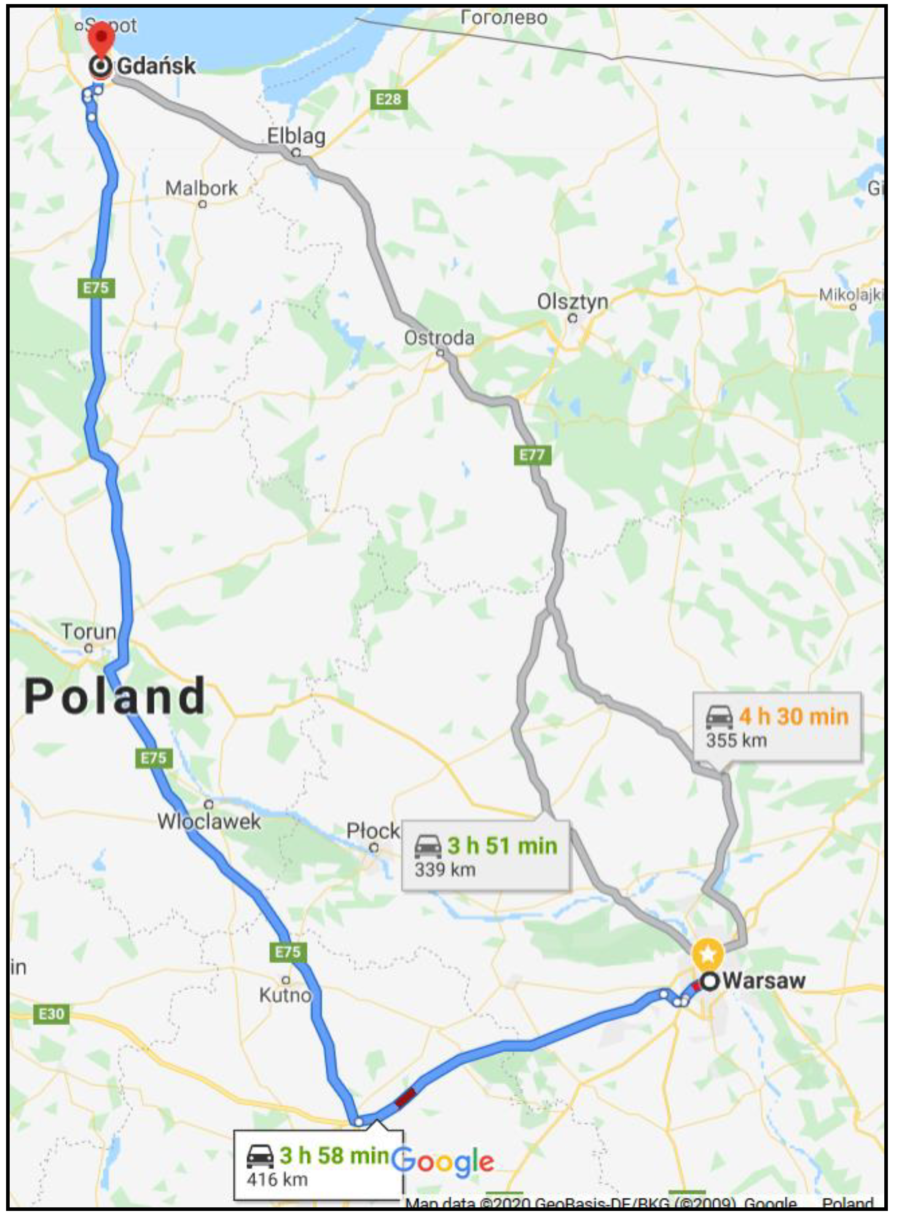
• Car connection from the Warszawa Centralna station area to the Gdansk Glowny station area via the A2 and A1 motorways—see Figure 3.

The communication route presented above can be shown using a graph as in Figure 4.

The individual connections (arcs in the graph) have the following characteristics—see

Table 1. Characteristics of individual connections.

No.	Arc	Mean of Transport	Distance [km]	Time [h]	Cost [USD/Person]
1	(1,2)	by foot	0.3	0.08	0.00
2	(1,3)	train	13.6	0.41	1.12
3	(1,4)	by foot	0.3	0.08	0.00
4	(2,5)	train	328.1	2.83	38.20
5	(3,6)	airplane	297.0	0.67	117.25
6	(4,7)	car	416.0	4.17	52.45
7	(5,8)	by foot	0.3	0.08	0.00
8	(6,8)	train	19.0	0.5	1.81
9	(7,8)	by foot	0.3	0.08	0.00

Source: our own work based on: https://www.google.pl/maps/, https://portalpasazera.pl/, https://www.wtp.waw.pl/, https://www.mazowieckie.com.pl/, https://bilet.intercity.pl/, https://www.flightradar24.com/, https://www.lot.com/, http://paliwo.ulewa.com/, http://www.skm.pkp.pl/, http://rss.nbp.pl/kursy/TabRss.aspx?n=2020/a/20a138.

. The cost of the trip is indicated for the day following the analysis—17.07.2020 r.

Additionally, due to the specificity of the analyzed route, the characteristics of individual graph vertices should be made—see

Table 2. Characteristics of individual graph vertices.

No.	Vertex	Place	Time [h]	Comments
1	1	Warszawa Centralna—main hall	0.00	Place of departure
2	2	Warszawa Centralna—platform	0.08 *	Place of boarding the train
3	3	Warszawa Okecie Airport	1.00 **	Place of transfer from train to airplane
4	4	Warszawa Centralna—car park	0.08 ***	Place of getting into the car
5	5	Gdansk Glowny—platform	0.00 ****	Place of getting out of the train
6	6	Gdansk Rebiechowo	0.33 *****	Place of transfer from airplane to train
7	7	Gdansk Glowny—car park	0.08 ******	Place of getting out of the car
8	8	Gdansk Glowny—main hall	0.00	Place of arrival

Note: * it was assumed that passengers arrive at platform 5 min before departure; ** it was assumed that for domestic flights the time to perform activities at the airport before departure is 1 h; *** it was assumed that preparing the driver for driving will take 5 min; **** it was assumed that upon arrival the passenger goes straight to the station hall; ***** it was assumed that for domestic flights the time of performing activities at the airport after arrival is 20 min; ****** it was assumed that securing the vehicle upon arrival would take the driver 5 min; Source: own work.

.

Based on the above-mentioned details, it is possible to comprehensively characterize the travel variants. The characteristics are presented in

Table 3. Characteristics of individual travel variants.

Variant	The Main Means of Transport	Distance [km]	Time [h]	Cost [USD/Person]
1	train	328.7	3.08	38.20
2	airplane	329.0	2.91	120.18
3	car	416.0	4.33	52.45

Source: own work.

.

Considering the distance of the journey in the analyzed route, the train journey is the rational choice from the point of view of the adopted criterion, but the difference between the next solution—by airplane is only equal to 0.3 km. The least favorable distance is for the car connection. In terms of travel time, the airplane is the rational choice from the point of view of the adopted criterion, but the difference from the train connection is 0.17 h, which is about 10 min. The car connection is also the worst one among the analyzed variants. In terms of costs, rail transport is the rational choice from the point of view of the adopted criterion, but this time there is a huge difference compared to air transport—over 8150 USD (two Pendolino trips). Considering the number of changes in the case of air transport, it can be concluded that the rational choice from the point of view of all of the adopted criteria is to travel by train.

5.3. Distribution of the Traffic Flow in Analyzed Communication Route

It is reasonable to check how the traffic flow is distributed into individual connections from the point of view of the emission of harmful compounds. The example is limited to carbon dioxide only. To do this, it is necessary to perform additional parameterization—we need to define capacity and the amount of emission for individual arcs. These data are summarized in

Table 4. Additional characteristics of individual connections.

No.	Arc	Mean of Transport	Capacity [pas./day]	Unit Emission Volume [g/pas.]
1	(1,2)	by foot	∞	-
2	(1,3)	train	7884 *	166
3	(1,4)	by foot	∞	-
4	(2,5)	train	6184 *	10,438
5	(3,6)	airplane	342 *	41,140
6	(4,7)	car	30,000 *	50,128
7	(5,8)	by foot	∞	-
8	(6,8)	train	4785 *	303
9	(7,8)	by foot	∞	-

Note: pas = passengers. * The limitations related to the operation of public transport during the COVID-19 pandemic were considered. Source: own work based on: https://bilet.intercity.pl/, https://www.flightradar24.com/, https://www.lot.com/, https://forsal.pl, http://www.pkm-sa.pl/.

. It has been assumed that for a passenger car the emission value, in line with EU data from 2018, is 120.5 g/km [53]. Moreover, it was assumed that the occupancy rate of the car is one person per car. This value was assumed because the connections mainly used for business travel were analyzed. It is assumed that each driver drives his car and does not take anyone with him. The emission for air transport was determined on the basis of [54], and for railway transport on the basis of the method described in Section 4 of the article. Human carbon dioxide emissions from breathing have been neglected.

Additional characteristics of individual variants are presented in

Table 5. Additional characteristics of individual variants.

Variant	The Main Means of Transport	Capacity [pas./day]	Unit Emission Volume [g/pas.]
1	train	6184	10,438
2	airplane	342	41,609
3	car	30,000	50,128

Source: own work.

.

The distribution of the traffic flow was prepared using the Solver package built into Microsoft Excel. The solutions were searched using the evolutionary method with the limitation accuracy of 10⁻¹⁰. Convergence was assumed at the level of 10⁻⁷, and the mutation rate at the level of 0.075. The population size of initial solutions was 100 and the maximum time without recovery was 30 s. The results were scaled automatically. Maximum search time was limited up to 60 s.

The research was carried out according to the following methodology—different amounts of transport demand were checked, and we observed how many passengers should choose which means of transport. The test results are presented in

Table 6. Research of the distribution of the traffic flow on the network.

Demand Volume [pas./day]	100	1000	5000	6183	6184	6185	6525	6526	6527	10,000
train	100	1000	5000	6183	6184	6184	6174	6184	6184	6184
airplane	0	0	0	0	0	1	327	342	342	342
car	0	0	0	0	0	0	24	0	1	3474
Object. function [kg]	1044	10,438	52,190	64,538	64,549	64,590	79,253	78,779	78,829	25,2924

Source: own work.

.

Based on the research carried out, the following conclusions can be drawn. When distributing the traffic flow on the network from the point of view of carbon dioxide emissions by means of transport, it should be noted that until the transport capacity of trains is exhausted (6184 pas./day), the flow of traffic to be transported is entirely directed to means of rail transport. After this value is exceeded, passengers are directed to the airplane. As it approaches the limit, which is the sum of the capacity of trains and airplanes (6526 pas./day), the flow is directed to trains and airplanes. It should be noted that for a size of the flow one smaller than the aforementioned sum, it was directed in a slightly different way—the load on trains decreased by 10, on airplanes by 14, while the load on road transport appeared. After crossing the limit of the total capacity of trains and airplanes, the flow is directed to cars.

Finally, a chart will be presented showing the carbon dioxide emissions with the change in the size of the flow. It is shown in Figure 5.

On the basis of the many iterations of the distribution of the traffic flow into the analyzed communication route carried out, a function was developed that allows the calculation of the emission volume for a given route (y) depending on the amount of transport demand (x). It is as follows—formula (11):

$$y=20.057x-34055{\left[\frac{\mathrm{pas}.}{\mathrm{day}}\right]}_{.}$$

(11)

The R² coefficient for this formula is 0.7095. It is not very high value. According to the authors, the value of the coefficient could be improved by conducting more experiments for different volumes of transport demand.

Summing up, for the problem formulated in this way, railway transport is the most advantageous from the point of view of carbon dioxide emissions. This choice coincides with the considerations carried out regarding the selection of the rational choice from the point of view of the adopted criteria: time, cost and distance.

6. Conclusions

The problem of distributing the traffic flow on the transport network is very common in the literature. Researchers analyze all possible theories on the behavior of the traffic flow and use various methods to distribute the traffic flow on the network. Among them, the most important are optimization methods and simulation methods. Special IT tools supporting the work of researchers are being prepared for both.

In the article, the authors focused their attention on the proecological distribution of the traffic flow, i.e., the one that is as environmentally friendly as possible. This work concerns carbon dioxide and its impact on the environment. The reason why this substance was selected for analysis was that it is one of the main factors of climate change. In addition, the European Union attaches great importance to reducing carbon dioxide emissions, including through legal regulations, therefore conducting research by the member states in this direction is justified.

The case study in this article was conducted for the Warszawa—Gdansk communication route. Three types of connections were analyzed: car, air and rail. Two types of analyses were carried out—the first without the use of optimization tools, and the second with the use of optimization tools. The first analysis was based on the selection of a rational variant of travel between Warszawa and Gdansk based on three criteria considered separately: distance, time and cost. From the point of view of the distance criterion, a rational option is to travel by train (length 328.7 km). The next choice would be air transport (length 329.0 km, compared to the rational solution, the length of the way is 0.3 km longer, which is an increase of about 0.001%). The last choice would be a car connection (length 416.0 km, compared to the rational solution, the length of this way is 87.3 km longer, which is an increase of about 26.56%). From the point of view of the time criterion, a rational option is to travel by plane (duration 2.91 h). Another choice would be rail transport (duration 3.08 h, compared to the rational solution, the travel time is 0.17 h longer, which is an extension of the journey by about 0.058%). The last choice would be a car connection (duration 4.33 h, compared to the rational solution, the travel time is 1.42 h longer, which is an extension of the journey by about 48.8%). From the point of view of the cost criterion, a rational option is to travel by train (cost 38.2 USD/passenger.). The next choice would be road transport (cost 52.45 USD/passenger., compared to the rational solution, the cost is 14.25 USD/passenger. higher, an increase of approximately 37.3%). The last choice would be a flight connection (cost 120.18 USD/passenger, compared to the rational solution the cost is 81.98 USD/passenger higher, which is an increase of about 214.61%). In conclusion, according to two criteria, the rational option is a rail connection. Only in the time criterion was the air connection indicated as a rational solution, but its length was only 0.17 h shorter than the railway connection. Therefore, it can be concluded that rail transport is a rational way to travel from Warszawa to Gdansk from the point of view of distance, cost and travel time.

The second type of analysis was to carry out considerations using the optimization tool. In this analysis, the adopted criterion was the minimization of carbon dioxide emissions during the transport. Several experiments for various volumes of transport demand were carried out and it was checked how the individual connections would be loaded for these volumes. From the point of view of one passenger, the lowest level of carbon dioxide emissions is characteristic of the railway connection (10,438 g/pas.), next by air transport (41,609 g/pas., about 31,252 g/pas. more than by rail transport (299.41%)) and then road transport (50,128 g/pas., about 39,690 g/pas. more than by rail transport (380.25%)). Therefore, the optimal solution from the point of view of the criterion of minimizing the total carbon dioxide emissions is the passenger’s choice of rail transport. By making subsequent attempts to distribute the traffic flow, it turned out that until the railway connection capacity was exhausted (6184 pas./day), the optimal solution was to direct all passengers to the railway connection. After exceeding this value, the optimal solution was to load the railway connection by 100% and to systematically load the air connection. After reaching the 100% load on the rail and air connection (6526 pas./day), the flow was directed to the car connection. Therefore, the optimal connection from the point of view of minimum carbon dioxide emissions is a railway connection and the railway network should be developed due to the highest environmental friendliness. It should also be noted that from the point of view of each criterion in both types of analysis, rail transport is the optimal (rational) solution.

The method presented in the article can be used to analyze any communication route consisting of any combination of means of transport. Based on the distance and additional parameters, you should first estimate the amount of carbon dioxide emissions and then distribute the traffic flow. Instead of carbon dioxide, other pollutants can be analyzed.