Regionally Divergent Patterns in Factors Affecting Municipal Waste Production: The Polish Perspective


Abstract
1. Introduction
2. Materials
2.1. Preliminarny Data Analysis
2.2. Potential Determinants of MW Volume in Poland
3. Methods
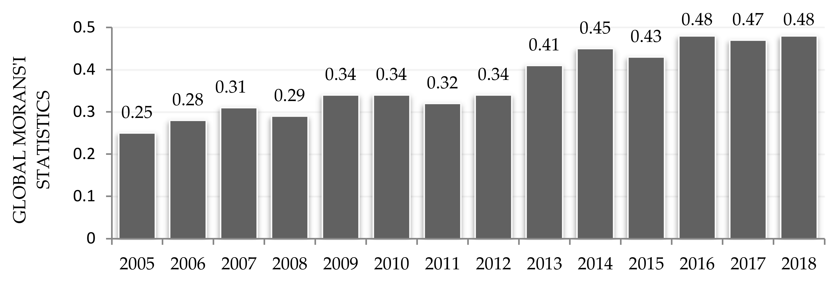
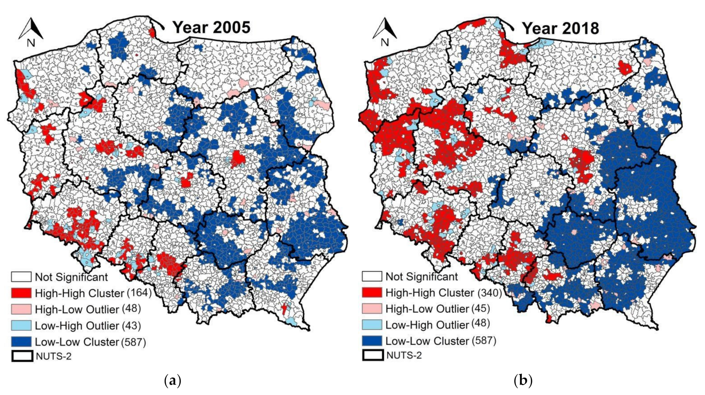
3.1. Moran’s I Spatial Autocorrelation Indices
3.2. Geographically Weighted Regression with Spatial Error Term
4. Results and Discussion
4.1. Spatial Dependencies in MW among Polish Communes
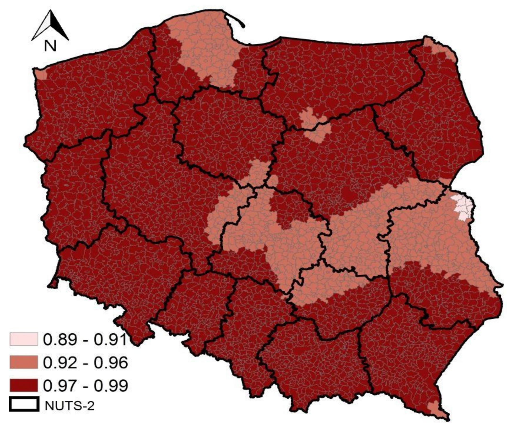
4.2. GWR–SEM Diagnostics
4.3. Modelling Results and Discussion
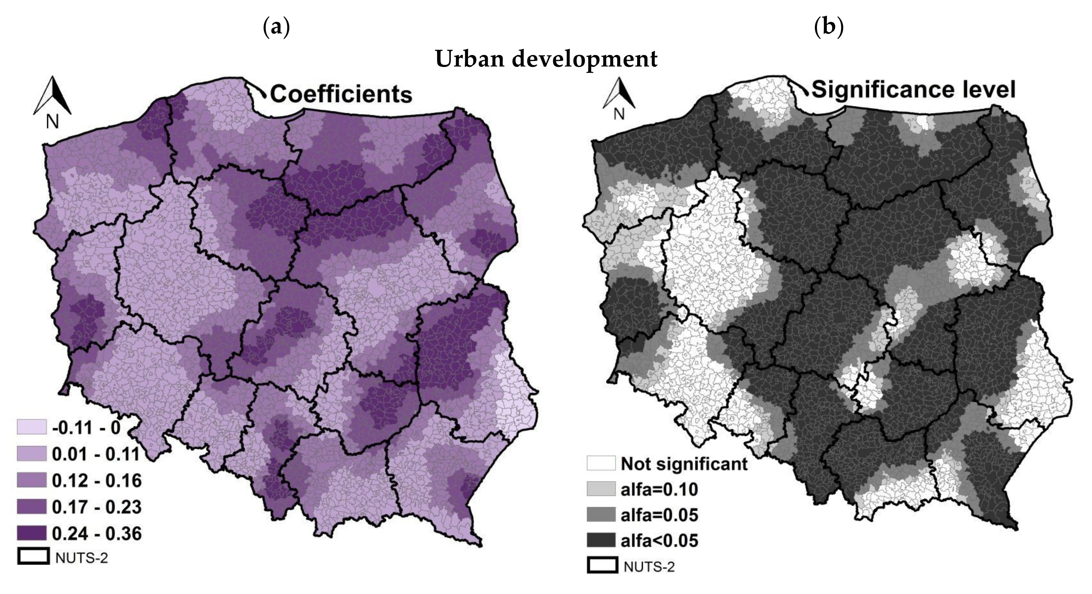
4.3.1. Urban Development
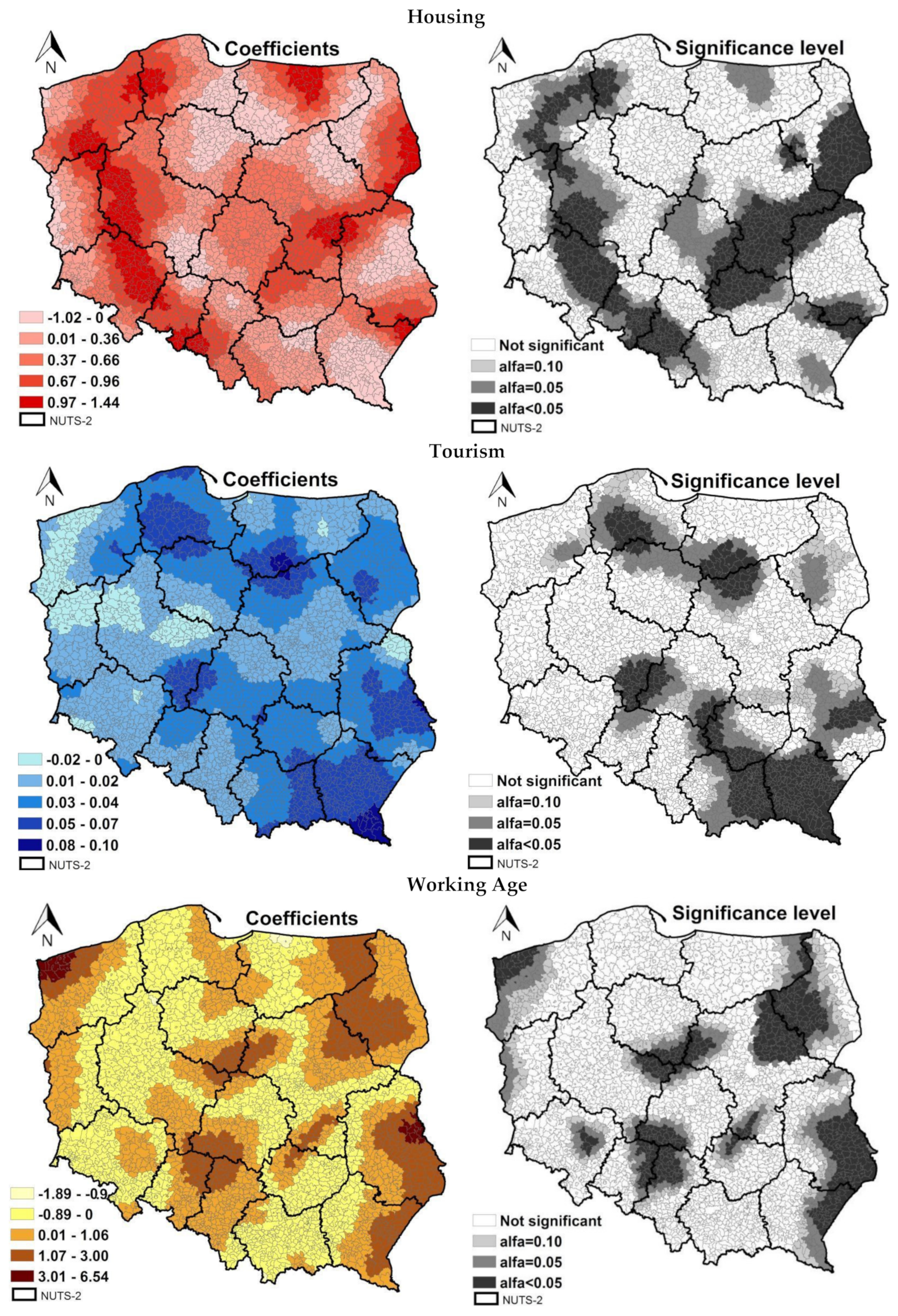
4.3.2. Housing
4.3.3. Tourism
4.3.4. Working Age
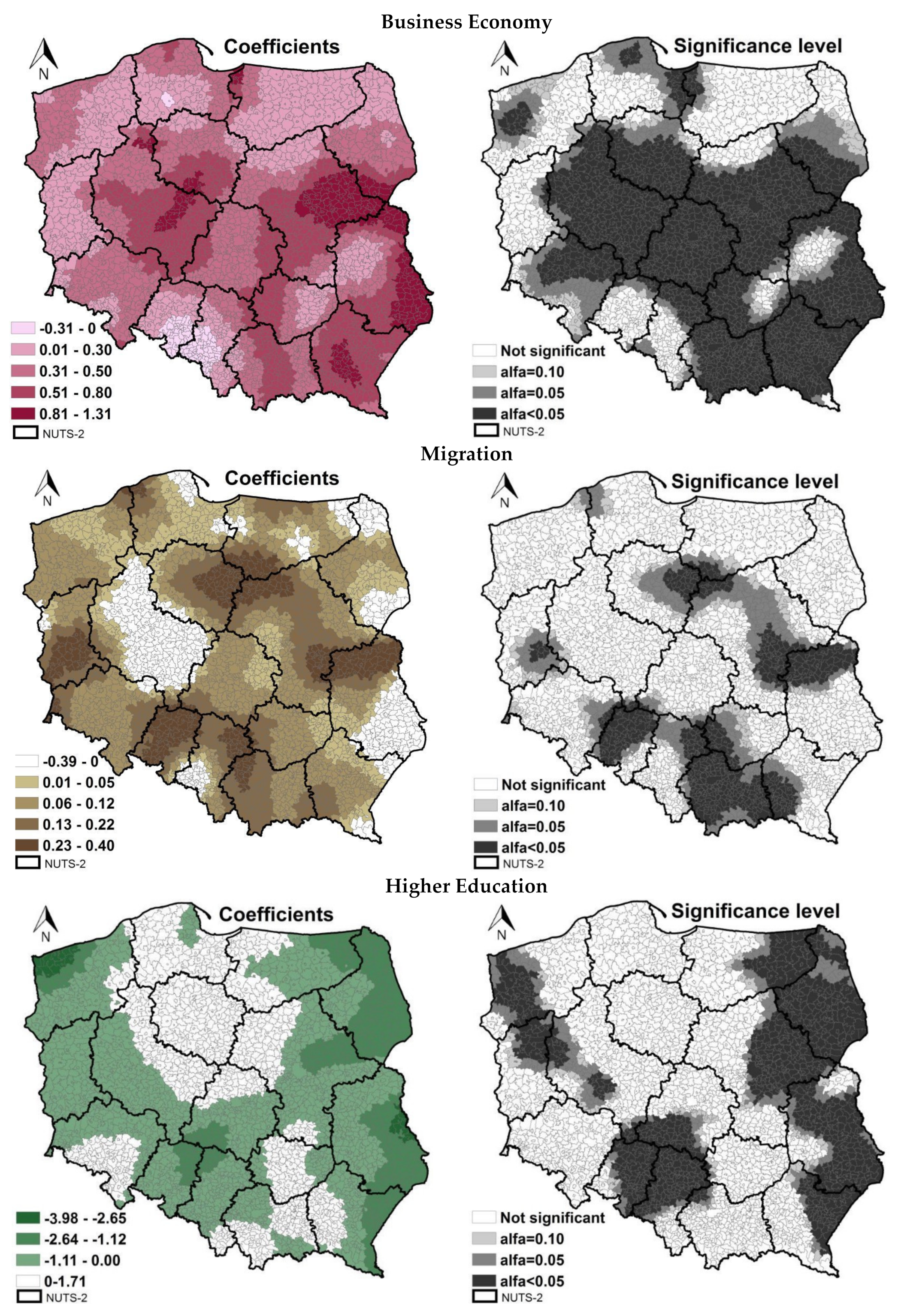
4.3.5. Business Economy
4.3.6. Migration
4.3.7. Higher Education
5. Conclusions
Author Contributions
Funding
Conflicts of Interest
Appendix A

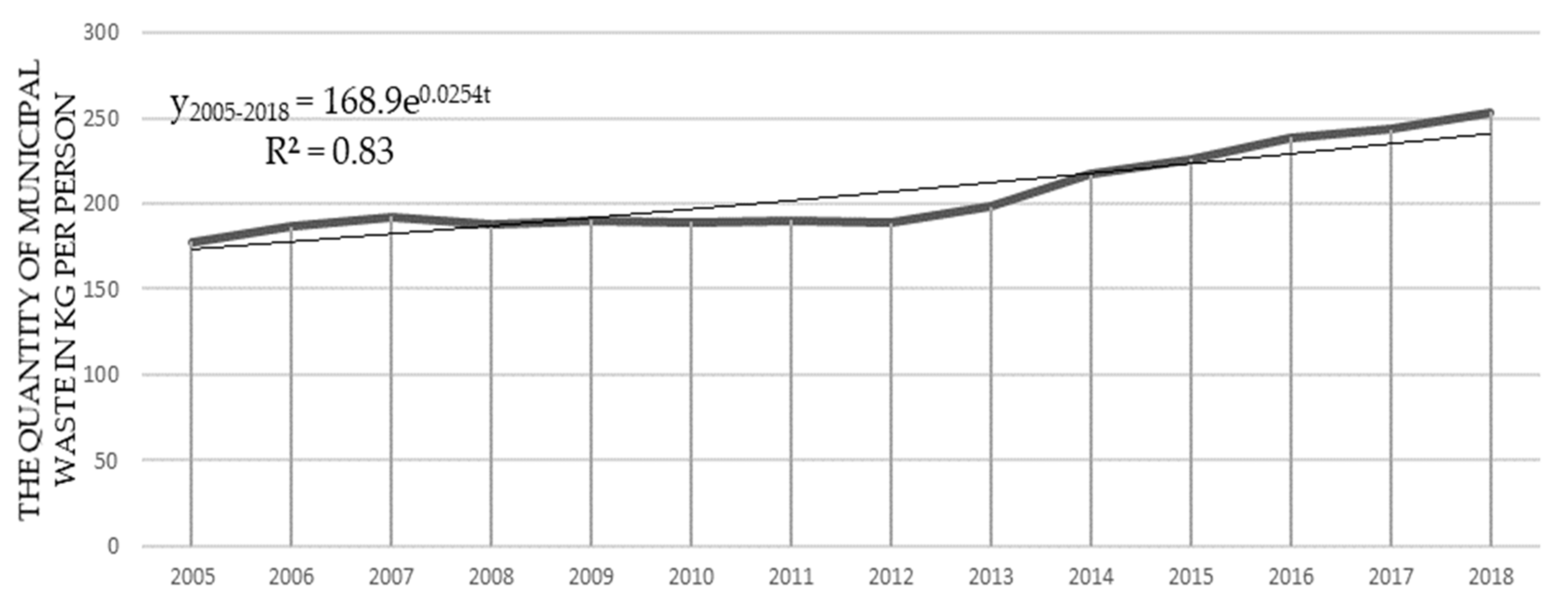
| Year | Mean | Median | Std. Dev. | Max | Min |
|---|---|---|---|---|---|
| 2005 | 178 | 132 | 85 | 484 | 1 |
| 2006 | 185 | 143 | 84 | 487 | 1 |
| 2007 | 191 | 152 | 83 | 527 | 1 |
| 2008 | 187 | 144 | 82 | 609 | 1 |
| 2009 | 189 | 148 | 84 | 694 | 1 |
| 2010 | 188 | 149 | 83 | 660 | 1 |
| 2011 | 189 | 154 | 77 | 598 | 1.3 |
| 2012 | 188 | 157 | 74 | 579 | 1.5 |
| 2013 | 197 | 174 | 70 | 613 | 5.8 |
| 2014 | 216 | 197 | 73 | 539 | 3.3 |
| 2015 | 225 | 209 | 75 | 949 | 4 |
| 2016 | 238 | 223 | 74 | 773 | 5.2 |
| 2017 | 246 | 227 | 74 | 773 | 6.3 |
| 2018 | 253 | 236 | 77 | 805 | 11 |
| Variable | Mean | Median | St. Dev. | Min | Max |
|---|---|---|---|---|---|
| UR | - | - | - | - | - |
| D | 315 | 307 | 51 | 202 | 864 |
| TO | 57 | 1 | 338 | 0 | 8913 |
| WA | 62.3 | 63 | 2.2 | 46.3 | 72.7 |
| EE | 1200 | 1075 | 514 | 189 | 6689 |
| M | 12 | 10 | 6 | 1 | 63 |
| ED | 105 | 103 | 19 | 66 | 141 |
| Variable | Mean | Median | St. Dev. | Min | Max |
|---|---|---|---|---|---|
| Intercept | −0.07 | −0.09 | 0.46 | −1.40 | 1.44 |
| UR | 0.13 | 0.13 | 0.07 | −0.11 | 0.36 |
| D | 0.40 | 0.43 | 0.42 | −1.02 | 1.44 |
| TO | 0.02 | 0.02 | 0.02 | −0.02 | 0.09 |
| WA | 0.22 | 0.05 | 0.87 | −1.89 | 6.54 |
| EE | 0.42 | 0.41 | 0.24 | −0.31 | 1.31 |
| M | 0.09 | 0.08 | 0.11 | −0.39 | 0.40 |
| ED | −0.33 | −0.18 | 0.77 | −5.98 | 1.71 |
References
- OECD. Municipal Waste. Available online: https://data.oecd.org/waste/municipal-waste.htm (accessed on 10 July 2020).
- Eurostat. Municipal Waste Statistics. Available online: https://ec.europa.eu/eurostat/statistics-explained/index.php/Municipal_waste_statistics#Municipal_waste_generation (accessed on 10 July 2020).
- European Environmental Agency. Eurostat: Environmental Data Centre on Waste. Available online: https://www.eea.europa.eu/themes/waste/links/eurostat-environmental-data-centre-on-waste (accessed on 10 July 2020).
- Eurostat. Waste-Overview. Available online: http://ec.europa.eu/eurostat/web/waste (accessed on 10 July 2020).
- Musmeci, L.; Bellino, M.; Cicero, M.R.; Falleni, F.; Piccardi, A.; Trinca, S. The impact measure of solid waste management on health: The hazard index. Annali dell’Istituto Superiore di Sanità 2010, 46, 293–298. [Google Scholar] [CrossRef] [PubMed]
- United Nations. Transforming Our World: The 2030 Agenda for Sustainable Development. Available online: https://sustainabledevelopment.un.org/post2015/transformingourworld (accessed on 10 July 2020).
- European Commission. Environment Action Programme to 2020. Available online: https://ec.europa.eu/environment/action-programme/ (accessed on 10 July 2020).
- United Nations. Sustainable Development Goals. Available online: https://www.un.org/sustainabledevelopment/wp-content/uploads/2019/01/SDG_Guidelines_AUG_2019_Final.pdf (accessed on 10 July 2020).
- Polish Local Data Bank of Central Statistical Office. Municipal Waste and Maintenance of Cleanliness and Order in Communes. Available online: https://bdl.stat.gov.pl/BDL/metadane/metryka/2840?back=True (accessed on 10 July 2020).
- Ministry of the Environment. Awareness, Attitudes and Ecological Behavior of Poles. Available online: https://www.mos.gov.pl/srodowisko/edukacja-ekologiczna/badania/badania-swiadomosci-ekologicznej/ (accessed on 10 July 2020). (In Polish)
- Pires, A.; Martinho, G.; Chang, N. Solid waste management in Europe countries: A review of systems analysis techniques. J. Environ. Manag. 2011, 92, 1033–1050. [Google Scholar] [CrossRef] [PubMed]
- Ministry of the Environment. Waste Management. Available online: https://www.mos.gov.pl/fileadmin/user_upload/mos/Aktualnosci/2017/grudzien_2017/Raport_z_badania_dot._gospodarki_odpadami__2017_r._.pdf (accessed on 10 July 2020). (In Polish)
- European Environment Agency. Municipal Solid Waste (MSW) Management and Selected Policy Instruments in European Countries, 2001–2015. Available online: https://www.eea.europa.eu/themes/waste/waste-management/municipal-waste-management-across-european-countries/table-3-1-municipal-solid (accessed on 10 July 2020).
- Alwaeli, M. An overview of municipal solid waste management in Poland. The current situation, problems and challenges. Environ. Prot. Eng. 2015, 41, 181–193. [Google Scholar] [CrossRef]
- Act amending the Act on Maintaining Cleanliness and Order in Communes and certain other acts (the “Draft Act”) amending Act of 13 September 1996 on Maintaining Cleanliness and Order in Communes (consolidated text-Journal of Laws of 2018, item 1454), the Act on Waste of 14 December 2012 (consolidated text-Journal of Laws of 2018, item 992) and the Act of 20 February 2015 on Renewable Energy Sources (consolidated text Journal of Laws of 2018, item 2389). Available online: https://www.linklaters.com/pl-pl/insights/publications/2019/march/planned-amendments-to-the-waste-act-in-poland (accessed on 24 August 2020).
- Przydatek, G. Assessment of changes in the municipal waste accumulation in Poland. Environ. Sci. Pollut. Res. 2020, 27, 25766–25773. [Google Scholar] [CrossRef] [PubMed]
- Boer Den, E.; Jędrczak, A.; Kowalski, Z.; Kulczycka, J.; Szpadt, R. A review of municipal solid waste composition and quantities in Poland. Waste Manag. 2010, 30, 369–377. [Google Scholar] [CrossRef]
- Smol, M.; Duda, J.; Czaplicka-Kotas, A.; Szołdrowska, D. Transformation towards Circular Economy (CE) in Municipal Waste Management System: Model Solutions for Poland. Sustainability 2020, 12, 4561. [Google Scholar] [CrossRef]
- Beigl, P.; Lebersorger, S.; Salhofer, S. Modelling municipal solid waste generation: A review. Waste Manag. 2008, 28, 200–214. [Google Scholar] [CrossRef]
- Bosire, E.; Oindo, B.; Atieno, J.V. Modeling Household Solid Waste Generation in Urban Estates Using SocioEconomic and Demographic Data, Kisumu City, Kenya. Available online: https://repository.maseno.ac.ke/handle/123456789/441 (accessed on 10 July 2020).
- Oribe-Garcia, I.; Kamara-Esteban, O.; Martin, C.; Macarulla-Arenaza, A.M.; Alonso-Vicario, A. Identification of influencing municipal characteristics regarding household waste generation and their forecasting ability in Biscay. Waste Manag. 2015, 9, 26–34. [Google Scholar] [CrossRef]
- Ramachandra, T.; Bharath, H.; Kulkarni, G.; Han, S.S. Municipal solid waste: Generation, composition and GHG emissions in Bangalore, India. Renew. Sustain. Energy Rev. 2018, 82, 1122–1136. [Google Scholar] [CrossRef]
- Sterner, T.; Bartelings, H. Household waste management in a Swedish municipality: Determinants of waste disposal, recycling and composting. Environ. Res. Econ. 1999, 13, 473–491. [Google Scholar] [CrossRef]
- Hage, O.; Söderholm, P. An econometric analysis of regional differences in household waste collection: The case of plastic packaging waste in Sweden. Waste Manag. 2008, 28, 1720–1731. [Google Scholar] [CrossRef] [PubMed]
- Kolekar, K.A.; Hazra, T.; Chakrabarty, S.N. A review on prediction of municipal solid waste generation models. Procedia Environ. Sci. 2016, 35, 238–244. [Google Scholar] [CrossRef]
- Vieira, V.H.A.D.M.; Matheus, D.R. The impact of socioeconomic factors on municipal solid waste generation in São Paulo, Brazil. Waste Manag. Res. 2018, 36, 79–85. [Google Scholar] [CrossRef] [PubMed]
- Prades, M.; Gallardo, A.; Ibàñez, M.V. Factors determining waste generation in Spanish towns and cities. Environ. Monit. Assess. 2015, 187, 4098. [Google Scholar] [CrossRef] [PubMed]
- Khan, D.; Kumar, A.; Samadder, S. Impact of socioeconomic status on municipal solid waste generation rate. Waste Manag. 2016, 49, 15–25. [Google Scholar] [CrossRef]
- Mateu-Sbert, J.; Ricci-Cabello, I.; Villalonga-Olives, E.; Cabeza-Irigoyen, E. The impact of tourism on municipal solid waste generation: The case of Menorca Island (Spain). Waste Manag. 2013, 33, 2589–2593. [Google Scholar] [CrossRef]
- Johnstone, N.; Labonne, J. Generation of household solid waste in OECD countries: An empirical analysis using macroeconomic data. Land Econ. 2004, 80, 529–538. [Google Scholar] [CrossRef]
- Sung, H.-C.; Sheu, Y.-S.; Yang, B.-Y.; Ko, C.-H. Municipal Solid Waste and Utility Consumption in Taiwan. Sustainability 2020, 12, 3425. [Google Scholar] [CrossRef]
- Caruso, G.; Gattone, S.A. Waste Management Analysis in Developing Countries through Unsupervised Classification of Mixed Data. Soc. Sci. 2019, 8, 186. [Google Scholar] [CrossRef]
- Shi, G.; Li, Q.; Zeng, D.; Zhang, Y.; Fei, Y.; Xie, Y. Influencing factors of domestic waste characteristics in rural areas of developing countries. Waste Manag. 2018, 72, 45–54. [Google Scholar] [CrossRef]
- Bach, H.; Mild, A.; Natter, M.; Weber, M. Combining socio-demographic and logistic fac tors to explain the generation and collection of waste paper. Res. Conser. Recyc. 2004, 41, 65–73. [Google Scholar] [CrossRef]
- Hockett, D.; Lober, D.J.; Pilgrim, K. Determinants of per capita municipal solid waste generation in the Southeastern United States. J. Environ. Manag. 1995, 45, 205–218. [Google Scholar] [CrossRef]
- Cheng, J.; Shi, F.; Yi, J.; Fu, H. Analysis of the factors that affect the production of municipal solid waste in China. J. Cleaner Produc. 2020, 259, 120808. [Google Scholar] [CrossRef]
- Tałałaj, I.A. The influence of chosen socio-economical factors on change of waste quantity in podlaskie province. Inżynieria Ekologiczna 2011, 25, 146. (In Polish) [Google Scholar]
- Generowicz, A. Multi-Criteria Analysis of Waste Management in Szczecin. Pol. J. Environ. Stud. 2014, 23, 57–63. [Google Scholar] [CrossRef]
- Cheba, K. Methods of forecasting changes in municipal waste production in case of cities. AUL Folia Oecon. 2014, 3, 223–229. [Google Scholar]
- Ulfik, A.; Nowak, S. Determinants of Municipal Waste Management in Sustainable Development of Regions in Poland. Pol. J. Environ. Stud. 2014, 23, 1039–1044. [Google Scholar]
- Kukuła, K. Municipal Waste Management in Poland in the Light of Multi-Dimensional Comparative Analysis. Acta Sci. Pol. Oeconomia 2016, 15, 93–103. [Google Scholar]
- Klojzy-Karczmarczyk, B.; Makoudi, S. Analysis of Municipal Waste Generation Rate in Poland Compared to Selected European Countries. 2017. Available online: www.e3s-conferences.org/articles/e3sconf/abs/2017/07/e3sconf_eems2017_02025/e3sconf_eems2017_02025.html (accessed on 7 July 2020).
- Keser, S.; Duzgun, S.; Aksoy, A. Application of spatial and non-spatial data analysis in determination of the factors that impact municipal solid waste generation rates in Turkey. Waste Manag. 2010, 32, 359–371. [Google Scholar] [CrossRef]
- Keser, S. Investigation of the Spatial Relationship of Municipal Solid Waste Generation in Turkey with Socio-Economic, Demographic and Climatic Factors. Available online: http://citeseerx.ist.psu.edu/viewdoc/download?doi=10.1.1.632.5116&rep=rep1&type=pdf (accessed on 10 July 2020).
- Antczak, E. Municipal Waste in Poland: Analysis of the Spatial Dimensions of Determinants Using Geographically Weighted Regression. Eur. Spat. Res. Policy 2019, 26, 177–197. [Google Scholar] [CrossRef]
- Rybova, K.; Burcin, B.; Slavík, J. Spatial and non-spatial analysis of socio-demographic aspects influencing municipal solid waste generation in the Czech Republic. Detritus 2018. [Google Scholar] [CrossRef]
- Rybova, K. Do Sociodemographic Characteristics in Waste Management Matter? Case Study of Recyclable Generation in the Czech Republic. Sustainability 2019, 11, 2030. [Google Scholar] [CrossRef]
- Antczak, E. Regional Patterns in Dumping Sites in Poland—Analysis in Context of the New “Sustainable” Waste Policy. Pol. J. Environ. Stud. 2020, 29, 1037–1049. [Google Scholar] [CrossRef]
- Kołsut, B. Inter-Municipal Cooperation in Waste Management: The Case of Poland. Quaest. Geogr. 2016, 35, 104–191. [Google Scholar] [CrossRef]
- Cyranka, M.; Jurczyk, M.; Pajak, T. Municipal Waste-to-Energy plants in Poland–current projects. In Proceedings of the E3S Web of Conferences, Kraków, Poland, 17–19 May 2016. [Google Scholar] [CrossRef]
- Anselin, L. Spatial Externalities, Spatial Multipliers, and Spatial Econometrics. Int. Reg. Sci. Rev. 2003, 26, 153–166. [Google Scholar] [CrossRef]
- Ismaila, A.B.; Muhmmed, I.; Bibi, U.M.; Husain, M.A. Modelling Municipal Solid Waste Generation Using Geographically Weighted Regression: A Case Study of Nigeria. Int. Res. J. Environ. Sci. 2015, 4, 98–108. [Google Scholar]
- European Commission. Background. Available online: https://ec.europa.eu/eurostat/web/nuts/background (accessed on 12 August 2020).
- European Commission. Local Administrative Units (LAU). Available online: https://ec.europa.eu/eurostat/web/nuts/local-administrative-units (accessed on 12 August 2020).
- Anselin, L.; Florax, R.J. New Directions in Spatial Econometrics; Springer Science & Business Media: Berlin, Germany, 1995. [Google Scholar]
- Getis, A.; Jared, A. Constructing the Spatial Weights Matrix Using a Local Statistic. Geogr. Anal. 2004, 36, 90–104. [Google Scholar] [CrossRef]
- Matthews, S.A.; Yang, T.C. Mapping the results of local statistics: Using geographically weighted regression. Demogr. Res. 2012, 26, 151–166. [Google Scholar] [CrossRef]
- Charlton, M.; Fotheringham, A.S. Geographically Weighted Regression; National Centre for Geocomputation: Maynooth, Ireland, 2009. [Google Scholar]
- Fotheringham, A.S.; Brunsdon, C.; Charlton, M. Geographically Weighted Regression: The Analysis of Spatially Varying Relationships; John Wiley & Sons: Hoboken, NJ, USA, 2003. [Google Scholar]
- Tobler, W. A computer movie simulating urban growth in the Detroit region. Econ. Geogr. 1970, 46, 234–240. [Google Scholar] [CrossRef]
- Fotheringham, A.S.; Brunsdon, C.; Charlton, M.E. Geographically Weighted Regression: The Analysis of Spatially Varying Relationships; Wiley: Chichester, UK, 2002. [Google Scholar]
- Fotheringham, A.S.; Brunsdon, C.; Charlton, M.E. Quantitative Geography: Perspectives on Spatial Data Analysis; Sage: London, UK, 2000. [Google Scholar]
- Loader, C.R. Bandwidth selection: Classical or plug-in? Ann. Stat. 1999, 27, 415–438. [Google Scholar] [CrossRef]
- Bowman, A. An Alternative Method of Cross-Validation for the Smoothing of Density Estimate. Biometrika 1984, 71, 353–360. [Google Scholar] [CrossRef]
- Gollini, I.; Lu, B.; Charlton, M.; Brunsdon, C.; Harris, P. GWR model: An R Package for Exploring Spatial Heterogeneity Using Geographically Weighted Models. J. Stat. Softw. 2015, 63, 1–50. [Google Scholar] [CrossRef]
- Ferré, J. Regression Diagnostics; Comprehensive Chemometrics; Brown, S.D., Tauler, R., Walczak, B., Eds.; Elsevier: Amsterdam, The Netherlands, 2009; pp. 33–89. [Google Scholar] [CrossRef]
- Marquardt, D.W. Generalized inverses, ridge regression, biased linear estimation and nonlinear estimation. Technometrics 1970, 12, 591–612. [Google Scholar] [CrossRef]
- Andy, M. The ESRI Guide to GIS Analysis. Volume 2: Spatial Measurements and Statistics and Zeroing. In Geographic Information Systems at Work in the Community; ESRI Press: Boston, MA, USA, 2005. [Google Scholar]
- Leung, Y.; Mei, C.L.; Zhang, W.X. Statistical Tests for Spatial Nonstationarity Based on the Geographically Weighted Regression Model. Environ. Plan. Econ. Space 2000, 32, 9–32. [Google Scholar] [CrossRef]
- Cho, S.H.; Lambert, D.M.; Roberts, R.K.; Kim, S.G. Demand for Open Space and Urban Sprawl: The Case of Knox County, Tennessee. In Progress in Spatial Analysis. Advances in Spatial Science (The Regional Science Series); Páez, A., Gallo, J., Buliung, R., Dall’erba, S., Eds.; Springer: Berlin/Heidelberg, Germany, 2010. [Google Scholar]
- Lewandowska-Gwarda, K.; Antczak, E. Urban Ageing in Europe—Spatiotemporal Analysis of Determinants. ISPRS Int. J. Geo-Inf. 2020, 9, 413. [Google Scholar] [CrossRef]
- Akinwande, M.O.; Dikko, H.G.; Samson, A. Variance Inflation Factor: As a Condition for the Inclusion of Suppressor Variable(s) in Regression Analysis. Open J. Stat. 2015, 5, 754–767. [Google Scholar] [CrossRef]
- Hervé, A.L.; Williams, J.L. Principal Component Analysis. WIREs Comput. Stat. 2010, 2, 433–459. [Google Scholar]
- Yu, D.-L. Spatially varying development mechanisms in the Greater Beijing area: A geographically weighted regression investigation. Ann. Reg. Sci. 2006, 40, 173–190. [Google Scholar] [CrossRef]
- Jenkins, R.R. The Economics of Solid Waste Reduction; Edward Elgar Publishing Limited: Aldershot, UK, 1993. [Google Scholar]
- World Bank. Urban Development. Available online: https://data.worldbank.org/topic/urban-development?end=2019&locations=PL&start=2003&view=chart (accessed on 13 July 2020).
- Becker, S.O.; Boeckh, K.; Hainz, C.; Woessmann, L. The Empire Is Dead, Long Live the Empire! Long-Run Persistence of Trust and Corruption in the Bureaucracy. Econ. J. 2016, 126, 40–74. [Google Scholar] [CrossRef]
- Bukowski, P. How history matters for student performance: Lessons from the Partitions of Poland. J. Comp. Econ. 2018, 47, 136–175. [Google Scholar] [CrossRef]
- Hlaváček, P.; Kopáček, M.; Horáčková, L. Impact of Suburbanisation on Sustainable Development of Settlements in Suburban Spaces: Smart and New Solutions. Sustainability 2019, 11, 7182. [Google Scholar] [CrossRef]
- Friedman, A. Fundamentals of Sustainable Dwellings; Joan, W., Ed.; Island Press: Washington, DC, USA, 2012. [Google Scholar]
- Local Data Bank of Polish Central Statistical Office. Housing Economy and Municipal Infrastructure. Available online: https://bdl.stat.gov.pl/BDL/metadane/cechy/szukaj?slowo=dwellings (accessed on 15 July 2020).
- European Commission. Regional Innovation Monitor Plus. Available online: https://ec.europa.eu/growth/tools-databases/regional-innovation-monitor/base-profile/podlaskie (accessed on 15 July 2020).
- National Polish Bank. Convergence and differentiation processes in local markets and structural changes (comparison of 16 markets in Poland). Available online: https://www.nbp.pl/publikacje/materialy_i_studia/174_en.pdf (accessed on 15 July 2020).
- Karwinska, A.; Böhm, A.; Kudłacz, M. The phenomenon of urban sprawl in modern Poland: Causes, effects and remedies. Zarządzanie Publiczne 2018, 26–43. [Google Scholar] [CrossRef]
- European Environmental Agency. European Briefings—Tourism. Available online: http://www.eea.europa.eu/soer-2015/europe/tourism (accessed on 15 July 2020).
- European Commission. Best Environmental Management Practice in the Tourism Sector. Available online: https://ec.europa.eu/environment/emas/takeagreenstep/pdf/BEMP-6-FINAL.pdf (accessed on 16 July 2020).
- Local Data Bank of Polish Central Statistical Office. Tourist Accommodation Establishments and Their Occupancy. Available online: https://bdl.stat.gov.pl/BDL/metadane/cechy/szukaj?slowo=tourism (accessed on 16 July 2020).
- Abram, M.; Sleboda, M. Directions the Development of Business Tourism in Poland-Issues of Sustainability. ECOCYCLES 2016, 2, 35–43. [Google Scholar] [CrossRef][Green Version]
- Baum, S. The Tourist Potential of Rural Areas in Poland. East. Eur. Countrys. Sciendo 2011, 17, 107–135. [Google Scholar] [CrossRef]
- Local Data Bank of Polish Central Statistical Office. Population at Pre-Working (up to the Age of 17), Working and Post-Working Age by Sex. Available online: https://bdl.stat.gov.pl/BDL/metadane/cechy/szukaj?slowo=working (accessed on 17 July 2020).
- Ciżkowicz, P.; Ciżkowicz-Pękała, M.; Pękała, P.; Rzońca, A. The Effects of Special Economic Zones on Employment and Investment: Spatial Panel Modelling Perspective. Economic Institute. National Polish Bank. 2015. Available online: https://www.nbp.pl/publikacje/materialy_i_studia/208_en.pdf (accessed on 17 July 2020).
- Jaroszewicz, M. Migration from Ukraine to Poland the Trend Stabilises. 2018. Available online: https://www.osw.waw.pl/sites/default/files/Report_Migration%20from%20Ukraine_net.pdf (accessed on 17 July 2020).
- Local Data Bank of Polish Central Statistical Office. Entities of the National Economy, Ownership and Structural Transformations. Available online: https://bdl.stat.gov.pl/BDL/metadane/cechy/szukaj?slowo=REGON (accessed on 18 July 2020).
- Operational Programme Eastern Poland 2014–2020. Available online: https://www.polskawschodnia.gov.pl/media/10302/POPW_english_version.pdf (accessed on 18 July 2020).
- European Commission. Warsaw Capital Region. Available online: https://ec.europa.eu/growth/tools-databases/regional-innovation-monitor/base-profile/warsaw-capital-region (accessed on 18 July 2020).
- Rees, P.; Bell, M.; Kupiszewski, M.; Kupiszewska, D.; Ueffing, P.; Bernard, A.; Charles-Edwards, E.; Stillwell, J. The Impact of Internal Migration on Population Redistribution: An International Comparison. Popul. Space Place 2017, 23, 2036. [Google Scholar] [CrossRef]
- Ilnicki, D. Rural Areas as the Origin and Destination of Permanent Internal Migrations between 2002 and 2017 in Poland. A Local-Level Analysis (Nuts 5). Quaest. Geogr. 2020, 39, 15–30. [Google Scholar] [CrossRef]
- Cieślińska, B.; Dziekońska, M. The Ideal and the Real Dimensions of the European Migration Crisis. The Polish Perspective. Soc. Sci. 2019, 8, 314. [Google Scholar] [CrossRef]
- Potrykowska, A. Population changes and internal migrations in Mazowieckie voivodship. Mazowsze Studia Regionalne 2018, 11–28. [Google Scholar] [CrossRef]
- Zaman, A.U. A Strategic Framework for Working toward Zero Waste Societies Based on Perceptions Surveys. Recycling 2017, 2, 1. [Google Scholar] [CrossRef]
- OECD. Better Life index. Poland. Available online: http://www.oecdbetterlifeindex.org/countries/poland/ (accessed on 20 July 2020).


| Variable | Description | Time Span | Category |
|---|---|---|---|
| UDS | Uncontrolled dumping sites per 100 km2 | 2008–2018 | Awareness/human development |
| PD | Population density in people per 1 km2 | 2005–2018 | Demography |
| WA | Population at the working age in % | 2005–2018 | Demography/ economy/human development |
| M | Registrations for permanent residence per 1000 people | 2005–2017 | Migration |
| TO | Nights spent by tourists per 1000 people | 2005–2018 | Tourism |
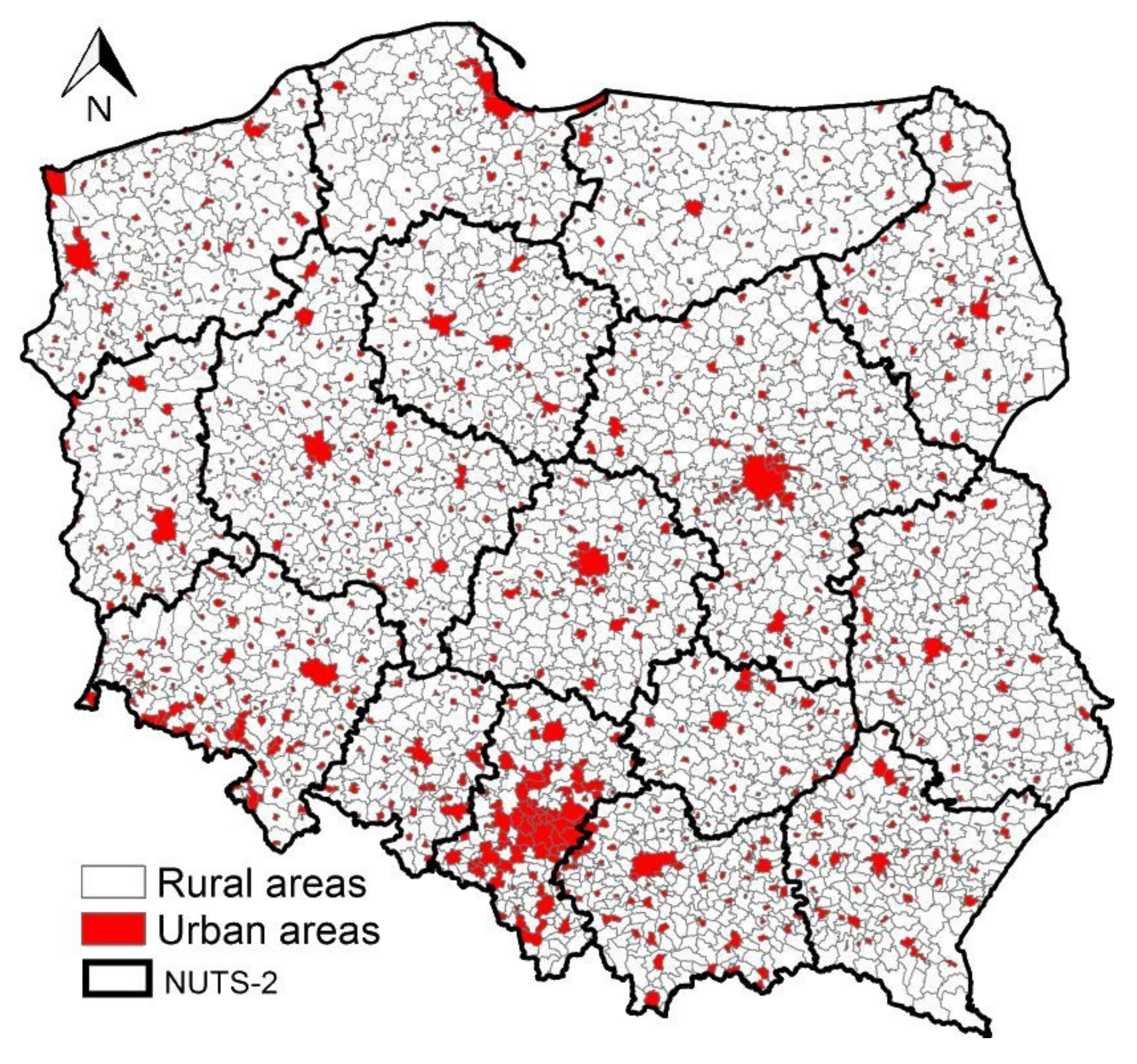
| UR | Urban and rural area: 2—urban areas, 1—rural areas | 2005–2018 | Urbanization/urban development/urban morphology |
| D | Dwelling stocks per 1000 population | 2005–2017 | Dwellings and housing/living conditions |
| MA | Permanent marketplaces of retail sales per 100,000 people | 2005–2017 | Sales retail/ consumption |
| EE | Entities of the national economy entered in the REGON system per 10,000 people | 2005–2017 | Economy/ development |
| ED | Higher education graduates per 10,000 people | 2005–2018 | Education/ awareness/human development |
| IN | Investments in waste municipal management system in PLN per capita | 2005–2018 | Investments/ economy |
| URP | Proportion of urban and rural population in % | 2005–2018 | Urbanization/ demography |
| IM | Infant mortality rate as the number of deaths per 1000 live births of children under one year of age | 2005–2018 | Demography/ living condition/health |
| LE | Life expectancy in years at age 0 | 2005–2018 | Demography/living condition/health |
| Variable | Coefficient | Standard Error | t-Student | VIF |
|---|---|---|---|---|
| Intercept | −8.93 *** | 0.57 | −15.78 | - |
| UR (urban/rural) | 0.11 *** | 0.01 | 10.15 | 2.3 |
| D (dwellings) | 0.50 *** | 0.06 | 8.04 | 1.6 |
| TO (tourism) | 0.02 *** | 0.004 | 4.93 | 1.3 |
| WA (working age) | 4.9 *** | 0.27 | 17.54 | 1.8 |
| EE (entities) | 0.41 *** | 0.03 | 12.82 | 2.4 |
| M (migration) | 0.13 *** | 0.02 | 5.50 | 1.3 |
| ED (education) | −0.19 *** | 0.04 | −4.39 | 1.1 |
| Diagnostics | OLS | GWR | GWR–SEM |
|---|---|---|---|
| Bandwidth | - | 26,635.3 | 34,636.4 |
| R-Squared | 0.54 | 0.77 | 0.98 |
| Adjusted R-Squared | 0.52 | 0.76 | 0.97 |
| Residual Sum of Square | 102.9 | 58.3 | 51.4 |
| AIC | −1692.4 | −2808.9 | −2859.5 |
| Moran’s I | 0.39 *** | 0.09 *** | 0.005 |
| Koenker (BP) Statistic | 14,120 *** | - | - |
| Jarque–Bera Statistics | 198.3 *** | 3.34 | 2.17 |
© 2020 by the author. Licensee MDPI, Basel, Switzerland. This article is an open access article distributed under the terms and conditions of the Creative Commons Attribution (CC BY) license (http://creativecommons.org/licenses/by/4.0/).
Share and Cite
Antczak, E. Regionally Divergent Patterns in Factors Affecting Municipal Waste Production: The Polish Perspective. Sustainability 2020, 12, 6885. https://doi.org/10.3390/su12176885
Antczak E. Regionally Divergent Patterns in Factors Affecting Municipal Waste Production: The Polish Perspective. Sustainability. 2020; 12(17):6885. https://doi.org/10.3390/su12176885
Chicago/Turabian StyleAntczak, Elżbieta. 2020. "Regionally Divergent Patterns in Factors Affecting Municipal Waste Production: The Polish Perspective" Sustainability 12, no. 17: 6885. https://doi.org/10.3390/su12176885
APA StyleAntczak, E. (2020). Regionally Divergent Patterns in Factors Affecting Municipal Waste Production: The Polish Perspective. Sustainability, 12(17), 6885. https://doi.org/10.3390/su12176885