Passenger Flow Prediction Based on Land Use around Metro Stations: A Case Study

Abstract

High-density land uses cause high-intensity traffic demand. Metro as an urban mass transit mode is considered as a sustainable strategy to balance the urban high-density land uses development and the high-intensity traffic demand. However, the capacity of the metro cannot always meet the traffic demand during rush hours. It calls for traffic agents to reinforce the operation and management standard to improve the service level. Passenger flow prediction is the foremost and pivotal technology in improving the management standard and service level of metro. It is an important technological means in ensuring sustainable and steady development of urban transportation. This paper uses mathematical and neural network modeling methods to predict metro passenger flow based on the land uses around the metro stations, along with considering the spatial correlation of metro stations within the metro line and the temporal correlation of time series in passenger flow prediction. It aims to provide a feasible solution to predict the passenger flow based on land uses around the metro stations and then potentially improving the understanding of the land uses around the metro station impact on the metro passenger flow, and exploring the potential association between the land uses and the metro passenger flow. Based on the data source from metro line 2 in Qingdao, China, the perdition results show the proposed methods have a good accuracy, with Mean Absolute Percentage Errors (MAPEs) of 11.6%, 3.24%, and 3.86 corresponding to the metro line prediction model with Categorical Regression (CATREG), single metro station prediction model with Artificial Neural Network (ANN), and single metro station prediction model with Long Short-Term Memory (LSTM), respectively.

1. Introduction

With the rapid socio-economic development in China, China has experienced urbanization on a scale unprecedented in recent decades. Urbanization leads to high-density development of land use in urban areas for the increasing population. High-density land uses cause high-intensity traffic demand. Land use and transport are hot topics within sustainable transportation in China, as they are undergoing a major demographic transition of rapid and intense urbanization [1]. As to relieve the burden of traffic network for high-intensity traffic demand, the public transport leading oriented development is considered as a rational and sustainable strategy to balance the urban high-density land use development and the high-intensity traffic demand. Metro, with the advantages of being efficient, smooth, green, safe, large-volume, and land-saving, is the first choice of transport mode which is developing in many metropolises all over the world [2].

Metro, as a sustainable urban transport mode, has been expanding aggressively in recent decades. It attracts lots of residents and is taken as the first choice of trip mode for most commuters in many metropolises, such as Beijing, Shanghai, and Tokyo [3]. However, the capacity of metro always cannot meet the traffic demand during the rush hours. These phenomena cause traffic congestion within metro vehicles and metro stations, which lead to stampede accidents, being shut in the door, falling into the pathway, burglary, and other social problems. It calls for traffic agents to reinforce the operation and management standard by some advanced public transport technologies, to improve the service quality and increase the passenger travel shares rate of metro.

As to improving the operation and management standard of urban public transport system, researchers have developed kinds of mathematical models to explore the influence factors and relationships in the development and operation of public transport system. Kalantari [4] used the user planning support model to evaluate the potential relationship between public transport and the areas needed for future urban development. Holst [5] used a standard forecasting model to study the prediction of public transport passenger flow in sparsely populated areas and discussed their applicability. Corolli [6] used a heuristic method of problem structure to consider the random factors affecting the passenger demand in air traffic flow management. Ortuzar and willumsen [7,8], concerned with the interface between the decision-maker and the transport system, developed mental and mathematical models to assist the decision-maker to improve transport system management skills.

Passenger flow prediction is considered the foremost and pivotal technology in improving the management standard and service level of metro, as well as other public transport modes. In the area of passenger flow prediction for public transport, the mathematical prediction models that the researchers have used can be divided into linear models and nonlinear models, as far as we know. With linear models, the empirical data are mainly used to predict passenger flow under theoretical assumptions and specific condition parameters. Linear time series model [9], historical average model [10], nearest neighbor model [11], and error component model [12] are the kind of linear models which are used to infer the trend of passenger flow in some scenarios with specific theoretical assumptions. Xue [13] used the linear time series model to predict the short-term passenger flow of public transport, and the results showed that the time series model has defects in predicting the short-term passenger flow and it is more suitable for predicting the long-term passenger flow. The nonlinear models, such as nonlinear time series model [14,15], support vector machine model [16], and neural network model [17,18], are considered to have more accuracy in describing the characteristics of transit systems and better performance than linear models in passenger flow prediction. Castro [19] used a support vector machine model to predict traffic flow under typical and atypical traffic conditions and achieved better prediction results.

In the aspect of data use in passenger flow prediction, to our best knowledge, the state-of-the-art researches on passenger flow prediction for urban public transport in the libraries were mostly based on the historical data of Integrated Circuit (IC) cards. A series of machine learning models based on IC card data were used to explore the residents’ trip choice behavior and transit trip pattern for decision-making support in transit operation and management. The algorithms in these machine learning models can be divided into two groups as conventional statistical-based methods [13,20,21] and computational intelligence-based methods [22,23,24]. Wei [25] combined empirical mode decomposition with back propagation neural network to predict short-term passenger flow. The results showed that the prediction accuracy of the neural network is better than that of the Autoregressive Integrated Moving Average (ARIMA) model and Seasonal Autoregressive Integrated Moving Average (SARIMA) model. Yang [26] concluded that the Artificial Neural Network (ANN) model has the highest accuracy and shortest training time in evaluating passenger flow compared with several conventional statistical algorithms and computational intelligence algorithms.

Machine learning and deep learning frameworks such as TensorFlow, PyTorch, Keras were developed and applied in engineering. The neural network is becoming increasingly mature in research and easier to use in application, including in the area of traffic engineering. Ou [27] and Zhang [28] used the convolutional neural network to predict the origin-destination flow of traffic networks. Long Short-Term Memory (LSTM) neural network and Gated Recurrent Unit (GRU) were developed to capture the time dependence of time series in different time periods, and the research indicates that these models have excellent performance in the field of traffic flow prediction [21,29,30,31]. Yang [32] enhanced the LSTM model and compared with the conventional LSTM and Recurrent Neural Network (RNN), the experimental results showed that the training time and accuracy of the proposed model had a better performance. The researchers used LSTM and ANN to predict the traffic flow in different applications. They found that the LSTM model has the capability of effectively capturing the long-term and short-term characteristics of traffic flow and achieves higher accuracy in prediction compared with other algorithms [33,34,35].

In the aspect of land use development, it is well known that urban mass transit, such as light rail, Bus Rapid Transit (BRT), and metro, will increase the value of land use along the transit line [36,37]. Some researchers focus on the commercial investment based on the location of metro stations and land use [38,39,40,41]. Jian [42] studied the relationship of land use and metro passenger flow within a 500 m radius around the metro station in Osaka, Japan, and found that urban commercial building tends to be more dense when its location is closer to the metro station. Lin [43] explored the impact of the location of metro stations impacting on the customer flow of the shopping malls, and found out that there is a multi-relationship among the land price, the construction of the metro station, and the customer flow. Zheng [44] found that new metro station has a positive impact on the number and diversity of the catering services which are near the metro station. Izanloo [45] used the secondary data analysis method to determine the impact of commercial land on the number of trips. The results show that there is a strong correlation between commercial land and traffic flow.

From the perspective of investment economic, there is a potential association between the land uses around metro station and the metro passenger flow. To the best of our knowledge, there is little research on the metro passenger flow prediction based on the land uses. The analysis of the potential relationship between land uses around the metro station and the metro passenger flow is important for metro passenger flow prediction. This paper attempts to predict the metro passenger flow based on the relationship between land uses and metro stations. The main work of this paper focuses on:

(1)

Using mathematical and neural network modeling methods to predict metro passenger flow based on the land uses around the metro stations, along with considering the spatial correlation of metro stations within the metro line and the temporal correlation of time series in passenger flow prediction, and then exploring the potential association between the land uses and the metro passenger flow;

(2)

Providing a feasible solution to predict the passenger flow based on land uses around the metro stations and then potentially improving the understanding of the land uses around the metro station impact on the metro passenger flow, exploring the prediction procedure of the land uses to metro passenger flow.

The rest of this paper is organized as follows. Section 2 describes the data source used in this study, which includes the land uses data around the metro stations and the raw metro passenger flow data. Section 3 introduces the models of passenger flow prediction based on the metro line and single station. The effectiveness of the proposed model and its application are discussed in Section 4. Section 5 concludes this article with a summary of contributions and limitations, as well as the perspectives on future work.

2. Data Source

2.1. Metro Stations and Land Uses Data

In public transit station planning, a range with a radius of about 500 m is considered the suitable metro station service range [36,37]. It will take about 6–8 min walking to the metro station and it is acceptable and endurable by the residents [46]. Qingdao is a new modern city in China, and the urban construction had its vivid characteristics. It is a coastal, tourism, economically-developed, and major international port city in China. It has a typical and sound public transit network. The ridership of public transit is about 46%. The daily passenger flow of public transit is about 3 million. The 500 m coverage ratio of public transit stations is about 97%. The satisfaction rate of public transit passengers is higher than 92%. There are four open metro lines and four under construction metro lines, stretching the metro network to 327 km and likely boosting the average number of passengers to more than 419 thousand a day [47]. The land uses around the metro station almost cover all classification of land use, especially the metro line 2. Metro line 2 traverses the north-south urban high-density areas and the coastal route for tourism. The total length of metro line 2 is 25 km and is composed of 22 metro stations. There are three transfer stations within metro line 2. Licun station and Wusiguangchang station can transfer to metro line 3. Miaolinglu station can transfer to metro line 1. The layout of Qingdao metro network is shown in Figure 1.

In this paper, the land use data around the metro stations was obtained from the Qingdao Municipal Natural Resources and Planning Bureau [48]. Different colors indicate different land use properties. We matched the land uses within 500 m around each metro station of metro line 2, as shown in Figure 2.

As shown in Figure 2, within the service range of metro stations, the land use consists of residential land for urban residents, commercial and residential land, shopping mall and catering land, administrative office land, commercial service industry land, primary and secondary school land, village construction and residential land, sports land, green land, and other land properties. These types almost cover the land use classification in urban areas.

Google Earth Pro software (Google, CA, United States) can calculate the actual occupied area of various types of land uses according to the land uses planning by Qingdao Municipal Natural Resources and Planning Bureau. Figure 3 is an example of the mapping between Google Earth pro and the land uses. In the calculation process, a part of a certain land use property was included within 500 m radius of the metro station. We took all such land use properties into account, as shown in the area enclosed by the yellow line segment in Figure 3.

To simplify the analysis procedure, we classified the land uses into five types: Residential Land (RL), Entertainment and marketing Land (EL), Commercial Residence Land (CRL), School Land (SL), Administrative office Land (AL). The land use areas were calculated in square kilometers, as shown in

Table 1. The area of land use around the metro station.

Number	Metro Station	RL (km2)	EL (km2)	CRL (km2)	SL (km2)	AL (km2)
1	Taishanlu	0.20	0.00	0.16	0.05	0.10
2	Lijinlu	0.22	0.01	0.20	0.06	0.17
3	Taidong	0.23	0.01	0.21	0.04	0.15
4	Haixinqiao	0.14	0.01	0.02	0.07	0.12
5	Zhiquanlu	0.20	0.00	0.16	0.06	0.18
6	Wusiguangchang	0.22	0.01	0.22	0.04	0.10
7	Fushansuo	0.06	0.03	0.05	0.01	0.07
8	Yandaolu	0.13	0.01	0.13	0.01	0.07
9	Gaoxionglu	0.16	0.03	0.12	0.04	0.02
10	Maidaozhan	0.15	0.01	0.03	0.05	0.09
11	Haiyoulu	0.10	0.00	0.08	0.03	0.08
12	Haichuanlu	0.15	0.00	0.18	0.06	0.01
13	Haianlu	0.12	0.02	0.12	0.06	0.01
14	Shilaorenyuchang	0.16	0.02	0.13	0.03	0.02
15	Miaolinglu	0.08	0.01	0.07	0.10	0.00
16	Tonganlu	0.06	0.02	0.04	0.02	0.00
17	Liaoyangdonglu	0.01	0.02	0.01	0.00	0.02
18	Donghan	0.01	0.03	0.03	0.00	0.01
19	Hualoushanlu	0.01	0.02	0.02	0.01	0.01
20	Zaoshanlu	0.37	0.01	0.02	0.08	0.01
21	Licun	0.25	0.01	0.19	0.13	0.13
22	Licungongyuan	0.19	0.05	0.05	0.08	0.09

.

As shown in Table 1, it can be seen that the residential area around each metro station is higher than that of other land-use types, and the school area is positively correlated with the residential area, which meets the actual spatial layout of the city. It is worth noting that we just calculated the surface area of land uses from the map, not the buildings’ area.

In detail, it can be seen that the land uses around the metro stations have differences in type, composition, and proportion. This is in line with the layout characteristics of almost all urban metro stations and urban space structures. As there were different passenger flows in different metro stations which had different land uses around them, it is easy to link that there is a potential association between land use and passenger flow of the metro station.

2.2. Historical Metro Passenger Flow Data

In Qingdao metro, there is only one way to take the metro, which needs the IC card to be swiped in the entrance of the metro station. The IC card records the name and time of passengers entering and exiting the metro station. The raw IC card data contain the city code, IC card number, transaction date, transaction time, transaction type, and station code, which are used to identify the metro passenger flow. The snapshot of raw IC card data of the metro is shown as in

Table 2. The snapshot and sample of metro raw Integrated Circuit (IC) card data.

City Code	Card Number	Transaction Date	Transaction Time	Transaction Type	Station Code
2660	2660001342086610	1 July 2018	213152	8461	50000010016
2660	2660002200014080	6 July 2018	184020	8460	50000010015
2660	2660000000497220	1 July 2018	163811	8461	50000010022
2660	2660020000117840	5 July 2018	135317	8460	50000010005
2660	2660000000278000	1 July 2018	223142	8461	50000010022
2660	2660010000022250	1 July 2018	160051	8461	50000010015
2660	2660001322085800	1 July 2018	163631	8461	50000010201
2660	2660001312046720	1 July 2018	212652	8460	50000010004

. In the database, the transaction data and transaction time are recorded as eight-digit numbers and six-digit numbers, respectively. The formats of the transaction data and transaction time are “year-month-day” and “hour: minute: second”, which are missing the “-” or “:” in the number sequence, respectively. For example, “20180701” means 1 July 2018; “213152” means the time of 21:31:52. In the transaction type, “8460” indicates that the passenger entered the metro station; “8461” indicates that the passenger exited the metro station. We obtained one month of the raw IC card data of Qingdao metro line 2 from 1 to 31 July 2018.

3. Passenger Flow Prediction

3.1. Passenger Flow Prediction Based on the Line

3.1.1. Prediction Models

The occurrence and attraction of passenger flow around the metro station will be affected by the land uses around the metro station [42,49]. In this paper, we attempted to take the metro passenger flow in rush hours as the explanatory variable, and to take the area of land uses around the station as the explained variable, then form the incidence equation to analyze the areas of land use impacting on the metro passenger flow.

To explore the relationship between the passenger flow and the land uses around metro stations, we renamed the stations of Qingdao metro Line 2, Taishanlu to Licungongyuan as 1 to 22 in the analysis process. We selected the rush hours of metro passenger flow in each station from 2 to 6 July 2018 and from 9 to 13 July 2018 as the regression data. The rush hour in the morning is from 6:00 to 8:00. The rush hour in the evening is from 17:00 to 19:00.

These 10 days were two consecutive weeks of normal working days in July. In working days, commuter travel is more regular and stable, which makes it more reasonable for exploring the relationship between land uses and passenger flow. Figure 4 shows the rush hours passenger flow of each station in two consecutive weeks. The solid line represents the morning rush hour data and the dotted line represents the evening rush hour data.

The following can be seen from the metro passenger flow in Figure 4:

(1)

From the distribution of metro passenger flow in rush hours, the passenger flow distribution of each station is relatively stable and regular. For most metro stations, there is a big gap of metro passenger flow between the morning rush hour and evening rush hour.

(2)

In metro line 2, station 6, station 15, and station 21 are the transfer stations. It can be seen from Figure 4 that the passenger flow in the rush hours, especially in the morning rush hour, is larger. This paper used the data of card swiping within metro line 2. For transfer stations, passengers do not swipe their card again when they transfer. Therefore, the passenger flow of transfer stations had no effect on this study.

To further analyze the relationship between land use and metro passenger flow, the Categorical Regression (CATREG) method was used to fit the equations to evaluate the passenger flow. The optimal scale regression model was used to analyze the factors that affect the metro passenger flow during rush hours. Moreover, we set the metro passenger flow in the rush hours as the dependent variable, and the independent variable was Residential Land (RL), Entertainment and marketing Land (EL), Commercial Residence Land (CRL), School Land (SL), Administrative office Land (AL). All variables were put into the equation, and then the variables were deleted based on the correlation between land uses. That is, if the type of land use meets the elimination criteria, it will be eliminated until the equation meets the removal criteria. The structure of the equation is shown as Equation (1):

$$PF={\beta }_0+{\beta }_{1}RL+{\beta }_{2}EL+{\beta }_{3}CRL+{\beta }_{4}SL+{\beta }_{5}AL+\epsilon ,$$

(1)

where ${\beta }_0$ is a constant; ${\beta }_1, {\beta }_2, {\beta }_3, {\beta }_4, {\beta }_5$ are the coefficient parameters, respectively; $\epsilon$ is an error term.

First, the correlation between variables was checked and a bivariate correlation matrix was generated, as shown in

Table 3. The correlation coefficients between types of land uses.

Pearson Correlation	PF	RL	EL	CRL	SL	AL
PF	1.000	0.894	−0.633	0.634	0.495	0.883
RL	0.894	1.000	−0.543	0.849	0.523	0.703
EL	−0.633	−0.543	1.000	−0.457	−0.521	−0.517
CRL	0.634	0.849	−0.457	1.000	0.338	0.483
SL	0.495	0.523	−0.521	0.338	1.000	0.261
AL	0.883	0.703	−0.517	0.483	0.261	1.000

. The coefficient in Table 3 refers to the Pearson Correlation (PC) coefficient. The PC coefficients were used to test the correlation between the land uses around the metro station, in which the land use around the metro station was considered as an independent variable. To make sure the variables in the fitting equation were mutually independent, we could remove one of the variables which had a relatively strong correlation according to the coefficients in Table 3.

It can be seen from Table 3 that the absolute value of the correlation coefficient between the dependent variable PF and the independent variables RL, El, CRL, SL, Al was greater than 0.2, so the model can be further analyzed. The correlation coefficients between the independent variables RL and CRL were more than 0.8, which indicates that there is strong collinearity between the two variables, and it is unnecessary to keep the two variables at the same time. From the aspect of travel characteristics, the travel pattern of Residential Land (RL) includes the Commercial Residential Land (CRL). Therefore, we excluded Commercial Residential Land (CRL) from the independent variables.

With the IBM spss19.0 software (IBM, New York, United States), the relationship between the metro passenger flow and the land uses around the metro station was obtained. In this study, we chose the metro passenger flow during rush hour for further analysis. It can be seen from Figure 4 that the trend of passenger flow was basically the same. To get a more accurate fitting result, we fit the metro passenger flow using morning rush hour data and evening rush hour data. Then, we took the average value of the coefficients as the final coefficients.

In the process of fitting, we took the metro passenger flow during rush hour in 2 July 2018 as a case to analyze the fitting process, and the analysis process of the other nine days took the same process. As taking 2 July 2018 as the analysis object, the calibration results are shown in

Table 4. The coefficients based on morning rush hour data.

$\mathbf{Complex}\mathbf{Correlation}\mathbf{Coefficient}\mathbf{R}$	$\mathbf{Decision}\mathbf{Coefficient}{\mathbf{R}}^2$	$\mathbf{Correction}\mathbf{Coefficient}{\mathbf{R}}^2$	F	Sig.
0.970	0.941	0.925	56.240	0.001

and

Table 5. The coefficients based on evening rush hour data.

$\mathbf{Complex}\mathbf{Correlation}\mathbf{Coefficient}\mathbf{R}$	$\mathbf{Decision}\mathbf{Coefficient}{\mathbf{R}}^2$	$\mathbf{Correction}\mathbf{Coefficient}{\mathbf{R}}^2$	F	Sig.
0.797	0.634	0.530	6.076	0.005

.

According to the fitting results in Table 4 and Table 5, the correction coefficients of the two fitting results were greater than 0.4, which indicates that good results have been achieved by the fitting data. From the two fitting results, the significance of the t-test was less than 0.05, which indicates that the regression model obtained its statistical significance. The fitting results of the other nine days also received statistical significance.

According to the coefficient analysis results in

Table 6. The coefficients based on morning rush hour data.

Variate	Standardized Coefficients		t	Sig.	VIF
	B	Std. Error
Constant	75.594	77.177	0.979	0.344
RL	1925.609	444.818	4.329	0.001	2.633
EL	−2638.606	2609.258	−0.011	0.329	1.757
SL	948.016	966.160	0.981	0.343	1.671
AL	2560.570	499.039	5.131	0.001	2.249

Sig. is Significance; VIF is Variance Inflation Factor.

and

Table 7. The coefficients based on evening rush hour data.

Variate	Standardized Coefficients		t	Sig.	VIF
	B	Std. Error
(Constant)	927.731	447.984	2.071	0.057
RL	−2878.540	2582.007	−1.115	0.284	2.633
EL	−17,644.172	15,145.797	−1.165	0.264	1.757
SL	18,272.575	5608.209	3.258	0.006	1.671
AL	5755.952	2896.743	−1.987	0.067	2.249

, the Variance Inflation Factor (VIF) of each variable was less than 4, indicating that there was no collinear error among independent variables, and the overall fitting result of the equation was good. In statistics theory, when the independent variable Significance (sig.) is less than 0.05, it indicates that it is significant, and the fitting is significant.

From the fitting results of the morning rush hour and evening rush hour, almost all Sig. were greater than 0.05. On the one hand, the selected data volume was too small, only 19 groups. On the other hand, our statistical area only took the surface area, not the actual building area. Therefore, further analysis is needed.

The fitting results of the other nine groups of data are similar to those in Table 6 and Table 7, and they all meet the fitting conditions from the overall fitting results of the equation. Therefore, we consider the equation to be valid.

Through fitting the morning rush hour and evening rush hour passenger flow with 10 days of data and calculating the average value of coefficient, the final fitting equations of the morning rush hour and evening rush hour are as shown in Equations (2) and (3).

$$P{F}_{am}=1720.366RL-2288.84EL+1048.338SL+2297.089AL+81.375$$

(2)

$$P{F}_{pm}=-1682.56RL-14921.7EL+11666.85SL-4302.88AL+748.9939$$

(3)

It can be seen from the Equations (2) and (3) that:

(1)

In Equation (2), Residential Land (RL), School Land (SL), and Administrative office Land (AL) are in direct proportion to passenger flow. The passenger flow during the morning rush hour period is related to the concentration of residential area, which is reflected in our equation. Entertainment and catering Land (EL) is inversely proportional to the passenger flow, because entertainment and catering are not open during the morning rush hour period. However, the passenger flow of these places with large land area is smaller, which is in line with our expectation.

(2)

In Equation (3), the Administrative office land (AL) is directly proportional to the passenger flow. In the evening rush hour, it is the rush hour for students to leave school, and there are a large number of parents to pick up students. The large area of land produces a larger passenger flow, which is in line with the actual situation. School Land (SL), Residential Land (RL), Entertainment and catering Land (EL) are inversely proportional to passenger flow. The reason may be that most residents have not returned to their homes during the evening rush hour, and most residents choose to arrive rather than leave for restaurants and entertainment places. Therefore, the area of these three types of land uses is inversely proportional to the metro passenger flow.

3.1.2. Validation Analysis

To verify the accuracy of the fitting equation, we took the remaining stations 20, 21, 22 as the validation objects. This paper took the average value of morning rush hour and evening rush hour passenger flow of three stations as the actual value.

In this paper, the Mean Absolute Error (MAE) and the Mean Absolute Percentage Error (MAPE) were used to evaluate the final prediction accuracy [50]. MAE was used to evaluate the prediction bias at the level. MAPE was used to calculate the mean of the absolute differences between predictive and observed travel choices. Therefore, these two measures were used to evaluate the accuracy of prediction results. The Equations of MAE and MAPE are as Equations (4) and (5):

$$MAE=\frac{1}{n}{{\displaystyle \sum }}_i^n\left|y_i-\stackrel{\wedge }{y_i}\right|,$$

(4)

$$MAPE=\frac{1}{n}{{\displaystyle \sum }}_{i=1}^n\left|\frac{y_i-\stackrel{\wedge }{y_i}}{y_i}\right|\ast 100\%,$$

(5)

where $y_i$ is the actual passenger flow; ${\stackrel{\wedge }{y}}_i$ is the predicted passenger flow; $n$ is the sample size.

The error value of station passenger flow prediction is shown in

Table 8. The results of passenger flow prediction.

Station Number	Time	True Value	Predicted Value	MAE	MAPE
20	Morning rush hours	770	802	49	6.2%
21		1002	923
22		548	584
20	Evening rush hours	788	866	57	11.6%
21		583	540
22		279	230

.

It can be seen from Table 8 that the prediction errors of morning rush hours and evening rush hours were relatively small, which were within the acceptable range. At the same time, we found that the prediction results of the morning rush hour and evening rush hour were greater than the true value in metro station 20, while metro station 21 had the opposite results. However, the predicted value of the morning rush hour was greater than the real value, and the predicted value of the evening rush hour was less than the true value in metro station 22, which indicates that the prediction can roughly reflect the change of passenger flow, but the actual passenger flow will be affected by many other factors.

3.2. Passenger Flow Prediction Based on Metro Station

3.2.1. Prediction Models

Besides the spatial relationship among metro stations along the metro line, there is also a temporal relationship with time series in an independent metro station. The passenger flow of the metro station changes regularly in the working day. Figure 5 shows the change of passenger flow of station 20 within 10 working days, in which the statistics interval of passenger flow is 15 min.

We attempted to explore the potential relationship between the land uses around the metro station and the passenger flow based on the time series. The area of land uses around metro station 20 can be seen from the Table 2.

We took the passenger flow within 15 min interval as the dependent variable, and the area of land uses as the independent variable, to obtain the corresponding solution of land uses in each interval by linear programming method. The linear programming equation is as in Equation (6).

$$FL=x_{1}RL+x_{2}EL+x_{3}CRL+x_{4}SL+x_{5}AL$$

(6)

The source data in this analysis was the same as in Section 3.1, two consecutive weeks of 10 working days from 2 to 6 July 2018 and from 9 to 13 July 2018. The data interval was 15min, which was extracted from 06:00 to 21:00. Finally, we obtained 600 groups of passenger flow data.

The passenger flow of the metro station changes regularly with time-of-day, and the solutions of each land use obtained by linear programming are shown to be regular, correspondingly. The corresponding coefficients of land use in Equation (6) are shown in Figure 6.

To study the relationship between the temporal variation of passenger flow at a single station and the area of the land uses around the station, this paper used ANN and LSTM neural network to train and predict the corresponding coefficients of land use, and obtained the passenger flow of a single station in a certain period by the predicted coefficient plus its corresponding land use area as in Equation (6).

The LSTM network model was used to predict the passenger flow of the selected metro stations. LSTM is a kind of RNN, which can learn long-term dependence problems. RNN has a chain form of repetitive neural network modules. In a standard RNN, this repeating module has a very simple structure, such as a $\mathit{tan}h$ layer. Figure 7 shows the structure of RNN neural network and LSTM network.

Different from the traditional RNN, LSTM can remove or increase the ability of information to the cell state through a well-designed structure called a “gate”. The memory block in the LSTM network consists of four parts: input gate, output gate, forgetting gate, and storage unit. These three gates can determine what can be input, output, and forgotten in the training process. The storage unit is closely related to three gates, which can record and transmit useful historical information to the current task. The data flow can be calculated as in Equations (7)–(14):

$$f_t=\delta \left(W_f{x}_t+U_f{h}_{t-1}+V_f{c}_{t-1}+b_f\right),$$

(7)

$$i_t=\delta \left(W_i{x}_t+U_i{h}_{t-1}+V_i{c}_{t-1}+b_i\right),$$

(8)

$$\widetilde{c_t}=\mathit{tan}h(W_c{x}_t+U_c{h}_{t-1}+b_c),$$

(9)

$$c_t=f_t\ast c_{t-1}+i_t\ast {\tilde{c}}_t,$$

(10)

$$o_t=\delta \left(W_o{x}_t+U_o{h}_{t-1}+V_o{c}_t+b_o\right),$$

(11)

$$h_t=o_t\ast \mathit{tan}h(c_t),$$

(12)

$$\delta \left(x\right)=\frac{1}{1+e^{-x}},$$

(13)

$$\mathit{tan}h(x)=\frac{e^x-e^{-x}}{e^x+e^{-x}},$$

(14)

where $x_t,i_t,o_t,f_t,c_t,h_t$ represent the input data, input gate, output gate, forgetting gate, unit state, and final output, respectively; $W,U,V$ represent the weight matrixes, respectively; $b$ represents the deviation variable; the weight matrix and deviation vector $b$ need to be learned from the training data; $\delta \left(x\right)$ is the standard logic sigmoid function; $\mathit{tan}h\left(x\right)$ is a kernel function.

As the LSTM-based model takes the advantages of capturing the characteristics of long time series and short time series, we used LSTM to capture the characteristics of land use and solve the characteristics of medium-long time series and short time series to predict the metro passenger flow. The prediction process is shown in Figure 8.

In LSTM, there is a visible layer in LSTM, which has one input and seven LSTM neurons in the hidden layer. The output layer is used for single value prediction, and the activation function is the Rectified Linear Unit (ReLU). In the data training experiment, the prediction accuracy was not significantly promoted and fluctuated within a narrow range after 100 epochs in the training. The the system is considered to be in table status after 100 epochs. Therefore, the training time of LSTM was set as 100 epochs in the validation analysis.

3.2.2. Validation Analysis

As to verify the effective of LSTM, we used the data of metro station 20 in the validation analysis. There were 600 groups of raw data. In the prediction process, we used 70% for training and 30% for testing. ANN was used to compare the accuracy of the LSTM-based prediction. They shared the same raw data.

In ANN, the activation function is ReLU. The loss function is mean_squared_error, the optimizer is Adam. When it detects that loss stops improving, the training ends. To facilitate comparison, the training time of ANN was also set as 100 epochs. Figure 9 shows the predicted results of ANN and LSTM.

In the comparison, Mean Square Error (MSE) and Root Mean Square Error (RMSE) were used to reflect the accuracy of the two models.

Table 9. The prediction results of land use coefficient by ANN and LSTM.

		RL	EL	CRL	SL	AL
MSE	ANN	0.006438	0.006465	0.006449	0.006455	0.006487
	LSTM	0.006436	0.006435	0.006497	0.006483	0.006514
RMSE	ANN	0.080142	0.080541	0.080511	0.080396	0.080330
	LSTM	0.080245	0.080668	0.080468	0.080383	0.081420

shows the prediction results of land use coefficient by ANN and LSTM.

From the prediction results of the two machine learning algorithms, the error value is relatively small. It shows that the two machine learning methods have good performance in prediction of metro passenger flow and achieved higher prediction accuracy.

Table 10. The land use coefficients predicted by ANN.

Time	RL	EL	CRL	SL	AL
17:00–17:15	231.0916	6.2615	12.4550	50.1444	6.2250
17:15–17:30	242.0537	6.5611	13.0393	52.5533	6.5167
17:30–17:45	191.6175	5.1833	10.3514	41.4723	5.1748
17:45–18:00	187.2305	5.0635	10.1176	40.5087	5.0581
18:00–18:15	211.3574	5.7224	11.4032	45.8083	5.6999
18:15–18:30	165.2956	4.4645	8.9490	35.6908	4.4747
18:30–18:45	136.7802	3.6857	7.4297	29.4276	3.7162
18:45–19:00	125.8127	3.3862	6.8454	27.0187	3.4244

and

Table 11. The land use coefficients predicted by LSTM.

Time	RL	EL	CRL	SL	AL
17:00–17:15	229.5538	6.2736	12.6693	50.3783	6.3248
17:15–17:30	240.9808	6.5639	13.2494	52.7385	6.6355
17:30–17:45	189.5226	5.2102	10.5154	41.7264	5.2050
17:45–18:00	185.1876	5.0904	10.2698	40.7532	5.0807
18:00–18:15	209.3150	5.7454	11.6051	46.0794	5.7649
18:15–18:30	163.8742	4.4875	9.0227	35.8635	4.4604
18:30–18:45	137.1156	3.6953	7.3545	29.4768	3.6589
18:45–19:00	127.1258	3.3885	6.6987	27.0216	3.3528

show that land uses coefficients $x_1,x_2,x_3,x_4,x_5$ in Equation (6), which predicted by ANN and LSTM, respectively.

Based on the land use coefficients predicted by ANN and LSTM, the passenger flow could be predicted by Equation (6). The prediction results and the prediction errors are shown in

Table 12. The passenger flow predicted by ANN and LSTM.

Time	True Value	ANN			LSTM
		Predicted Value	MAE	MAPE	Predicted Value	MAE	MAPE
17:00–17:15	94	90	2.375	3.24%	89	2.875	3.86%
17:15–17:30	99	94			94
17:30–17:45	76	75			74
17:45–18:00	74	73			72
18:00–18:15	85	82			81
18:15–18:30	64	64			64
18:30–18:45	51	53			53
18:45–19:00	46	49			49
Evening rush hour	589	580	1.53%		576	2.21%

.

It can be seen from Table 12 that the prediction results of passenger flow using ANN and LSTM machine learning algorithms were accurate, and the prediction accuracy of ANN is higher than that of LSTM. From the prediction results of each time interval, the error was greater than that of the evening rush hours.

To show the prediction effects of ANN and LSTM model, the passenger flow in 13 July 2018 was taken as an example. According to the coefficient of each land type, the passenger flow predict results of the two models with a time interval of 15min were calculated and predicted. The results are shown in Figure 10.

It can be seen from Figure 10 that based on the whole day data comparison, the prediction results by ANN and LSTM all achieved good prediction results. The prediction results during rush hours were more accurate than peak hours.

It can see from the prediction results that the prediction accuracy of the ANN-based model is higher than that of LSTM. However, there is little difference in the prediction results of each coefficient, as shown in Table 10 and Table 11. Furthermore, in the actual prediction process, the learning rate of LSTM was much higher than that of ANN. In addition, although we just used 10-day data in training and analysis, there is a large amount of card data in practice and the learning rate is particularly much more important in practice situations with massive data. Therefore, we think that LSTM is better and suitable for capturing the long-term and short-term characteristics of IC card information in practice.

4. Discussion

From the existing research, we know that the passenger flow in the metro IC card data has temporal correlation and spatial correlation, and many factors affect metro passenger flow. In terms of space, in a period, the increase or decrease of the passenger flow is affected by the passenger flow input of adjacent stations. However, these influences will decrease as the distance increases. In terms of time, the passenger flow of the metro station will fluctuate with time, and the fluctuation trend is regular in a similar period. Furthermore, in different time periods, such as working days and holidays, the time-changing impact on metro passenger flow is not the same. Therefore, in the study of prediction of passenger flow, it is necessary to comprehensively consider the influence of spatial correlation and temporal correlation on metro station passenger flow. From the perspective of the whole metro line, there is spatial correlation between passenger flow information, and from a single metro station, the passenger flow information has time correlation with time. This paper started from the whole line and a single station, and explored the influence of space and time on station passenger flow.

Section 3.1 and Section 3.2 explored the relationship between the passenger flow and the land uses around the station from the whole line and the single station, respectively.

Section 3.1, based on the spatial correlation of the passenger flow at each station of the metro, carried out the equation with the passenger flow of the whole line and the land uses around the stations. In the fitting equation, to ensure accuracy, this paper chose the average value of the coefficients as the final coefficients of the equation. In the prediction process, we used the first 19 stations to fit the whole line equation and used the last three stations to verify the accuracy of the equation.

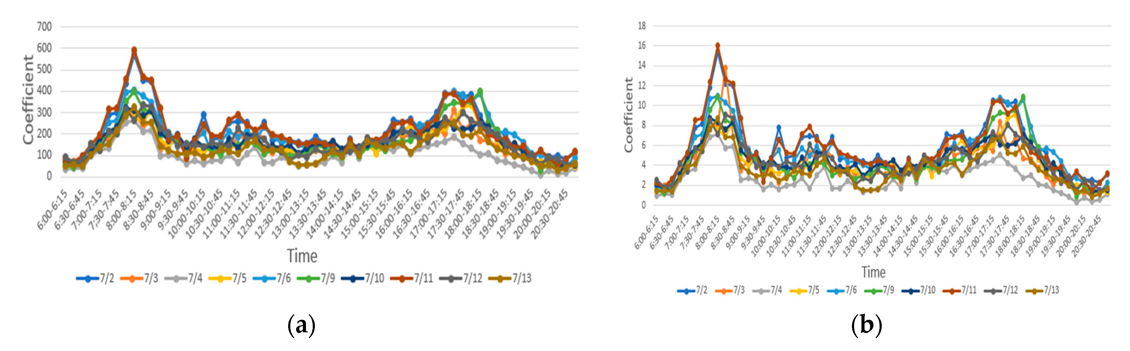
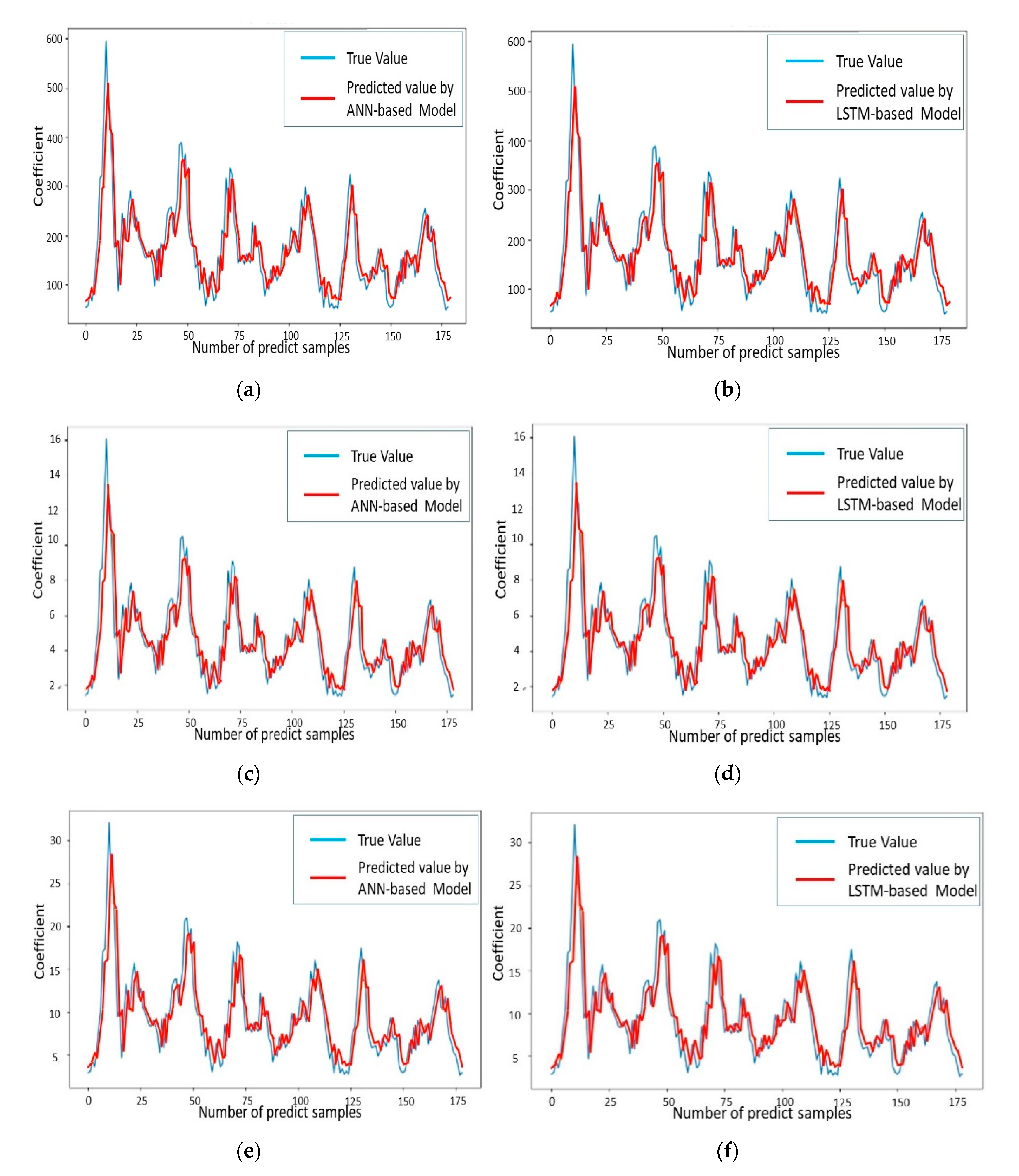
Section 3.2 was based on the temporal correlation between the passenger flow of a single metro station and the land uses around the station. In this section, we used metro station 20 as an example, using the passenger flow of two consecutive weekdays and selecting 15 min as the interval, and then obtain the coefficients of land use by using linear programming. The results show that the passenger flow and the coefficient are all changing along with time. ANN and LSTM were used for training the prediction.

Section 3.1 and Section 3.2 both forecast the passenger flow of evening rush hour for station 20. Based on whole line regression analysis, the predicted passenger flow of station 20 in morning rush hour was 866. The actual value of passenger flow was 788. The MAPE was 11.6%. Based on single station regression analysis and machine learning, the predicted passenger flow by ANN-based model and LSTM-based model were 580 and 576, respectively. The true value of passenger flow was 589. The MAPE was 3.24% and 3.86%, respectively. The MAE and MAPE of the prediction results by the ANN-based model and LSTM-based model were relatively small, both within the acceptable range. It can be inferred that there is a certain relationship between the passenger flow of the metro station and the land uses around the metro station.

At the same time, we also noticed that the accuracy of passenger flow prediction by using a single station is higher than that by using the whole line. There are two possible reasons for our analysis.

(1)

In the study of the whole line, the collinearity screening was made for land uses area when using the passenger flow and the land uses around the station, as shown in Table 3. After screening, the Commercial Residential Land (CRL) was eliminated, and only four types of land use were selected as variables. In the study of a single station, five types of land use were selected as the influencing factors, and the land uses were relatively rich so that more accurate prediction results were obtained.

(2)

In the study of the whole line, based on the prediction of metro station, the coefficient of the fitting equation was the average coefficient of 10 working days, and the average coefficient was used to predict, the error analysis was made between the prediction results and the average passenger flow of station 20 in 10 working days. However, in the study of single station, the selected passenger flow was the real value of daily passenger flow of 10 working days. Therefore, the prediction results and accuracy were in line with our expectations.

It can be concluded that there is a strong relationship between the passenger flow of the metro station and the land uses around the station. Compared with the whole line, considering the single station achieved more accurate prediction results. Therefore, in the study of metro passenger flow prediction, it is necessary to take the land uses around the station into account, and it is particularly important to take into account land uses around a single station.

5. Conclusions

In this paper, we used mathematical and neural network modeling methods to identify the relationship between the land uses around a metro station and the metro passenger flow. First, we used the categorical regression model to predict the metro passenger flow by considering the spatial relationships between the metro stations within the metro line. Then, Artificial Neural Network and Long Short-Term Memory were used to learn, train, and identify the coefficients of land use in the fitting equation. Based on the metro IC data during July 2018 and 500 m coverage of land uses around the stations along metro line 2, the prediction results show that the mean absolute percentage error of metro line prediction model with categorical regression, single metro station prediction model with artificial neural network, and single metro station prediction model with long short-term memory are 11.6%, 3.24%, and 3.86, respectively. From the effectives and results of the proposed model in this paper, we can conclude that:

(1)

The finding of this paper can be reconfirmed that there is an association between land use around a metro station and metro passenger flow. Metro passenger flow prediction based on single metro station with short time interval data and using the Artificial Neural Network method achieved higher accuracy and performance. Metro passenger flow prediction based on whole line metro station with rush hour data and using conventional regression method achieved higher accuracy than that of peak hours. It is considered that passenger flow prediction based on land use around metro station will get higher accuracy in using the spatial and temporal information synchronization;

(2)

The composition of land use around the metro station or along the metro line impacts on the passenger flow generation and the perdition accuracy. The more classifications of land use around the metro station, the higher accuracy will be obtained. The computational complexity and the neural network training time will increase sharply. It was found that the area of commercial residential land will affect the prediction accuracy randomly.

The aim of this paper was to explore the potential association between the land uses and the metro passenger flow, and potentially improve the understanding of the land uses around metro station impact on the metro passenger flow. However, the proposed method is not free from limitation. The first limitation is that we just considered the surface area of land use around the metro station. However, the land use intensity impacts the population density, which will generate metro travel demand. In addition, the value and location of land around the metro station affect the population density and transport mode choice of residents. They are the influences in metro passenger flow prediction. The second limitation is that the station number of other public transit modes was not considered. However, the condition and convenience of public transit network around the metro station will affect the attraction of metro trips by local residents. The third limitation is that the Origin-Destination (OD) of metro passengers was not used in the prediction model. The metro passenger flow is not only affected by the land uses around the metro station, but also by the OD of metro passengers.

These impactor factors and problems should be considered and added in further research. In the near future, further research work will focus on:

(1)

To improve the prediction accuracy, the influence range of the metro station should be identified instead of a 500 m radius range;

(2)

More factors affecting the metro travel demand and metro travel choice, such as weather, holidays, and resident distribution, should be included in the model modeling.

References

1. Zegras, C. Land Use and Transport in China. J. Transp. Land Use 2010, 3. [Google Scholar] [CrossRef] [Green Version]
2. Zhang, D.; Wang, X. Transit ridership estimation with network Kriging: A case study of Second Avenue Subway, NYC. J. Transp. Geogr. 2014, 41, 107–115. [Google Scholar] [CrossRef]
3. Wang, X.M.Y. Transit smart card data mining for passenger origin information extraction. J. Zhejiang Univ. Sci. C Comput. Electron. 2012, 13, 750–760. [Google Scholar]
4. Kalantari, Z.; Khoshkar, S.; Falk, H.; Cvetkovic, V.; Mortberg, U. Accessibility of Water-Related Cultural Ecosystem Services through Public Transport-A Model for Planning Support in the Stockholm Region. Sustainablity 2017, 9, 346. [Google Scholar] [CrossRef] [Green Version]
5. Holst, O. Accessibility as the objective of public transportation-planning—Integrated transportation and land-use model. Eur. J. Oper. Res. 1979, 3, 267–282. [Google Scholar] [CrossRef]
6. Corolli, L.; Lulli, G.; Ntaimo, L.; Venkatachalam, S. A two-stage stochastic integer programming model for air traffic flow management. IMA J. Manag. Math. 2017, 28, 19–40. [Google Scholar] [CrossRef]
7. De Dios Ortuzar, J.; Willumsen, L.G. Modelling Transport; John Wiley and Sons: Hoboken, NJ, USA, 2011. [Google Scholar] [CrossRef]
8. Willumsen, L.G.; de Dios Ortuzar, J. Intuition and models in transport management. Transp. Res. Part A Gen. 1985, 19, 51–57. [Google Scholar] [CrossRef]
9. Agafonov, A.A.; Myasnikov, V.V. An algorithm for traffic flow parameters estimation and prediction using composition of machine learning methods and time series models. Comput. Opt. 2014, 38, 539–549. [Google Scholar] [CrossRef]
10. El Esawey, M. Daily Bicycle Traffic Volume Estimation: Comparison of Historical Average and Count Models. J. Urban Plan. Dev. 2018, 144, 9. [Google Scholar] [CrossRef]
11. Wild, D. Short-term forecasting based on a transformation and classification of traffic volume time series. Int. J. Forecast. 1997, 13, 63–72. [Google Scholar] [CrossRef]
12. Frejinger, E.; Blerlaire, M. Capturing correlation with subnetworks in route choice models. Transp. Res. Part B Methodol. 2007, 41, 363–378. [Google Scholar] [CrossRef]
13. Xue, R.; Sun, D.; Chen, S.K. Short-Term Bus Passenger Demand Prediction Based on Time Series Model and Interactive Multiple Model Approach. Discret. Dyn. Nat. Soc. 2015, 11. [Google Scholar] [CrossRef] [Green Version]
14. Nikolopoulos, K.; Goodwin, P.; Patelis, A.; Assimakopoulos, V. Forecasting with cue information: A comparison of multiple regression with alternative forecasting approaches. Eur. J. Oper. Res. 2007, 180, 354–368. [Google Scholar] [CrossRef]
15. Smith, B.L.; Williams, B.M.; Oswald, R.K. Comparison of parametric and nonparametric models for traffic flow forecasting. Transp. Res. C Emer 2002, 10, 303–321. [Google Scholar] [CrossRef]
16. Angayarkanni, S.A.; Sivakumar, R.; Rao, Y.V.R. Hybrid Grey Wolf: Bald Eagle search optimized support vector regression for traffic flow forecasting. J. Ambient. Intell. Humaniz. Comput. 2020. [Google Scholar] [CrossRef]
17. Lau, K.W.; Wu, Q.H. Local prediction of non-linear time series using support vector regression. Pattern Recognit. 2008, 41, 1539–1547. [Google Scholar] [CrossRef]
18. Castro-Neto, M.; Jeong, Y.; Jeong, M.K.; Han, L.D. AADT prediction using support vector regression with data-dependent parameters. Expert Syst. Appl. 2009, 36, 2979–2986. [Google Scholar] [CrossRef]
19. Castro-Neto, M.; Jeong, Y.S.; Jeong, M.K.; Han, L.D. Online-SVR for short-term traffic flow prediction under typical and atypical traffic conditions. Expert Syst. Appl. 2009, 36, 6164–6173. [Google Scholar] [CrossRef]
20. Ma, X.L.; Wu, Y.J.; Wang, Y.H.; Chen, F.; Liu, J.F. Mining smart card data for transit riders’ travel patterns. Transp. Res. Part C Emerg. Technol. 2013, 36, 1–12. [Google Scholar] [CrossRef]
21. Jiang, X.; Zhang, L.; Chen, X. Short-term forecasting of high-speed rail demand: A hybrid approach combining ensemble empirical mode decomposition and gray support vector machine with real-world applications in China. Transp. Res. Part C Emerg. Technol. 2014, 44, 110–127. [Google Scholar] [CrossRef]
22. Tsai, T.-H.; Lee, C.-K.; Wei, C.-H. Neural network based temporal feature models for short-term railway passenger demand forecasting. Expert Syst. Appl. 2009, 36, 3728–3736. [Google Scholar] [CrossRef]
23. Li, H.Y.; Wang, Y.T.; Xu, X.Y.; Qin, L.Q.; Zhang, H.Y. Short-term passenger flow prediction under passenger flow control using a dynamic radial basis function network. Appl. Soft Comput. 2019, 83, 13. [Google Scholar] [CrossRef]
24. Wang, X.; An, K.; Tang, L.; Chen, X. Short Term Prediction of Freeway Exiting Volume Based on SVM and KNN. Int. J. Transp. Sci. Technol. 2015, 4, 337–352. [Google Scholar] [CrossRef] [Green Version]
25. Wei, Y.; Chen, M.C. Forecasting the short-term metro passenger flow with empirical mode decomposition and neural networks. Transp. Res. Part C Emerg. Technol. 2012, 21, 148–162. [Google Scholar] [CrossRef]
26. Li, Y.; Wang, X.; Sun, S.; Ma, X.; Lu, G. Forecasting short-term subway passenger flow under special events scenarios using multiscale radial basis function networks. Transp. Res. Part C Emerg. Technol. 2017, 77, 306–328. [Google Scholar] [CrossRef]
27. Ou, J.S.; Lu, J.W.; Xia, J.X.; An, C.C.; Lu, Z.B. Learn, Assign, and Search: Real-Time Estimation of Dynamic Origin-Destination Flows Using Machine Learning Algorithms. IEEE Access 2019, 7, 26967–26983. [Google Scholar] [CrossRef]
28. Zhang, J.L.; Chen, F.; Wang, Z.J.; Liu, H.X. Short-Term Origin-Destination Forecasting in Urban Rail Transit Based on Attraction Degree. IEEE Access 2019, 7, 133452–133462. [Google Scholar] [CrossRef]
29. Zhao, Z.; Chen, W.H.; Wu, X.M.; Chen, P.C.Y.; Liu, J.M. LSTM network: A deep learning approach for short-term traffic forecast. IET Intell. Transp. Syst. 2017, 11, 68–75. [Google Scholar] [CrossRef] [Green Version]
30. Zhang, D.; Kabuka, M.R. Combining weather condition data to predict traffic flow: A GRU-based deep learning approach. IET Intell. Transp. Syst. 2018, 12, 578–585. [Google Scholar] [CrossRef]
31. Tian, Y.X.; Pan, L. Predicting Short-term Traffic Flow by Long Short-Term Memory Recurrent Neural Network; IEEE: New York, NY, USA, 2015; pp. 153–158. [Google Scholar] [CrossRef]
32. Yang, D.; Chen, K.R.; Yang, M.N.; Zhao, X.C. Urban rail transit passenger flow forecast based on LSTM with enhanced long-term features. IET Intell. Transp. Syst. 2019, 13, 1475–1482. [Google Scholar] [CrossRef]
33. Zhao, J.; Qu, H.; Zhao, J.; Jiang, D. Towards traffic matrix prediction with LSTM recurrent neural networks. Electron. Lett. 2018, 54, 566–568. [Google Scholar] [CrossRef]
34. Cetiner, B.G.; Sari, M.; Borat, O. A neural network based traffic-flow prediction model. Math. Comput. Appl. 2010, 15, 269–278. [Google Scholar] [CrossRef]
35. Raza, A.; Zhong, M. Lane-based short-term urban traffic forecasting with GA designed ANN and LWR models. Transp. Res. Procedia 2017, 25, 1430–1443. [Google Scholar] [CrossRef]
36. Sohn, K.; Shim, H. Factors generating boardings at Metro stations in the Seoul metropolitan area. Cities 2010, 27, 358–368. [Google Scholar] [CrossRef]
37. Sung, H.; Oh, J.-T. Transit-oriented development in a high-density city: Identifying its association with transit ridership in Seoul, Korea. Cities 2011, 28, 70–82. [Google Scholar] [CrossRef]
38. Borjesson, M.; Isacsson, G.; Andersson, M.; Anderstig, C. Agglomeration, productivity and the role of transport system improvements. Econ. Transp. 2019, 18, 27–39. [Google Scholar] [CrossRef] [Green Version]
39. Debrezion, G.; Pels, E.; Rietveld, P. The impact of railway stations on residential and commercial property value: A meta-analysis. J. Real Estate Financ. Econ. 2007, 35, 161–180. [Google Scholar] [CrossRef] [Green Version]
40. Haddad, E.A.; Hewings, G.J.D.; Porsse, A.A.; Van Leeuwen, E.S.; Vieira, R.S. The underground economy: Tracking the higher-order economic impacts of the Sao Paulo Subway System. Transp. Res. Part A Policy Pract. 2015, 73, 18–30. [Google Scholar] [CrossRef]
41. Maghelal, P. Investigating the relationships among rising fuel prices, increased transit ridership, and CO2 emissions. Transp. Res. Part D Transp. Environ. 2011, 16, 232–235. [Google Scholar] [CrossRef]
42. Peng, J.; Peng, F.L.; Yabuki, N.; Fukuda, T. Factors in the development of urban underground space surrounding metro stations: A case study of Osaka, Japan. Tunn. Undergr. Space Technol. 2019, 91, 13. [Google Scholar] [CrossRef]
43. Lin, X.R.; Pan, H.X. The effects of the integration of metro station and mega-multi-mall on consumers’ activities: A case study of Shanghai. Transp. Res. Procedia 2017, 25, 2574–2582. [Google Scholar]
44. Zheng, S.Q.; Hu, X.K.; Wang, J.H.; Wang, R. Subways near the subway: Rail transit and neighborhood catering businesses in Beijing. Transp. Policy 2016, 51, 81–92. [Google Scholar] [CrossRef]
45. Izanloo, A.; Rafsanjani, A.K.; Ebrahimi, S.P. Effect of Commercial Land Use and Accessibility Factor on Traffic Flow in Bojnourd. J. Urban Plan. Dev. 2017, 143, 12. [Google Scholar] [CrossRef]
46. Serra-Coch, G.; Chastel, C.; Campos, S.; Coch, H. Graphical approach to assess urban quality: Mapping walkability based on the TOD-standard. Cities 2018, 76, 58–71. [Google Scholar] [CrossRef] [Green Version]
47. Bureau, Q.M.T. Qingdao Traffic Public Transportion Service Platform. Available online: http://qdjt.qingdao.gov.cn/n28356058/index.html (accessed on 14 August 2020).
48. Qingdao Natural Resources and Planning Bureau. Land Uses Planning. Available online: http://zrzygh.qingdao.gov.cn/n28356074/index.html (accessed on 1 March 2020).
49. Kim, D.; Ahn, Y.; Choi, S.; Kim, K. Sustainable Mobility: Longitudinal Analysis of Built Environment on Transit Ridership. Sustainability 2016, 8, 16. [Google Scholar] [CrossRef] [Green Version]
50. Lin, C.Y.; Wang, K.; Wu, D.Y.; Gong, B.W. Research on Residents’ Travel Behavior under Sudden Fire Disaster Based on Prospect Theory. Sustainability 2020, 12, 487. [Google Scholar] [CrossRef] [Green Version]
Figure 1. The snapshot of Qingdao metro network.
Sustainability 12 06844 g001
Figure 2. Land uses around metro stations. (a) Taishanlu station; (b) Lijinlu station; (c) Taidong station; (d) Haixinqiao station; (e) Zhiquanlu station; (f) Wusiguangchang station; (g) Fushansuo station; (h) Yandaolu station; (i) Gaoxionglu station; (j) Maidaozhan station; (k) Haiyoulu station; (l) Haichuanlu station; (m) Haianlu station; (n) Shilaorenyuchang station; (o) Miaolinglu station; (p) Tonganlu station; (q) Liaoyangdonglu station; (r) Donghan station; (s) Hualoushanlu station; (t) Zaoshanlu station; (u) Licun station; (v) Licungongyuan station; (w) legend of land use.
Sustainability 12 06844 g002aSustainability 12 06844 g002bSustainability 12 06844 g002c
Figure 3. The mapping and calculation process from Google Earth.
Sustainability 12 06844 g003
Figure 4. The passenger flow of metro station in the morning rush hours and evening rush hours.
Sustainability 12 06844 g004
Figure 5. The passenger flow of metro station 20.
Sustainability 12 06844 g005
Figure 6. The coefficients of land uses solved by linear programming. (a) Residential Land (RL) coefficients; (b) Entertainment and marketing Land (EL) coefficients; (c) Commercial Residence Land (CRL) coefficients; (d) School Land (SL) coefficients; (e) Administrative office Land (AL) coefficients.
Sustainability 12 06844 g006aSustainability 12 06844 g006b
Figure 7. The structure of Recurrent Neural Network (RNN) and Long Short-Term Memory (LSTM). (a) The structure of standard RNN; (b) The structure of LSTM.
Sustainability 12 06844 g007
Figure 8. The passenger flow prediction process based on LSTM.
Sustainability 12 06844 g008
Figure 9. Comparison of predicted and true values for each land uses coefficient. (a) RL coefficient predicted by ANN; (b) RL coefficient predicted by LSTM; (c) EL coefficient predicted by ANN; (d) EL coefficient predicted by LSTM; (e) CRL coefficient predicted by ANN; (f) CRL coefficient predicted by LSTM; (g) SL coefficient predicted by ANN; (h) SL coefficient predicted by LSTM; (i) AL coefficient predicted by ANN; (j) AL coefficient predicted by LSTM.
Sustainability 12 06844 g009aSustainability 12 06844 g009b
Figure 10. The results of passenger flow prediction by ANN and LSTM based model using the data of 13 July 2018.
Sustainability 12 06844 g010