Abstract
Faults in Heating, Ventilation and Air Conditioning (HVAC) systems affect the energy efficiency of buildings. To date, there rarely exist methods to detect and diagnose faults during the operation of buildings that are both cost-effective and sufficient accurate. This study presents a method that uses artificial intelligence to automate the detection of faults in HVAC systems. The automated fault detection is based on a residual analysis of the predicted total heating power and the actual total heating power using an algorithm that aims to find an optimal decision rule for the determination of faults. The data for this study was provided by a detailed simulation of a residential case study house. A machine learning model and an ARX model predict the building operation. The model for fault detection is trained on a fault-free data set and then tested with a faulty operation. The algorithm for an optimal decision rule uses various statistical tests of residual properties such as the Sign Test, the Turning Point Test, the Box-Pierce Test and the Bartels-Rank Test. The results show that it is possible to predict faults for both known faults and unknown faults. The challenge is to find the optimal algorithm to determine the best decision rules. In the outlook of this study, further methods are presented that aim to solve this challenge.
1. Introduction
In the effort to fight global warming, one of the German government’s goals is to achieve a climate-neutral building stock by 2050. The policies focus on two strategies, the use of renewable energies and the increase in energy efficiency. Long-term climate neutrality in the building sector can be achieved by reducing energy consumption and expanding renewable energy [1]. The thermal properties of the building envelope, the efficiency of building technology, and the user behaviour significantly influence energy efficiency of a building. In order to take measures to improve existing buildings, it is essential to detect the actual energy efficiency of a building. With on-site measurement data, the actual energy consumption can be detected, and flaws in energy efficiency identified.
Deviations from the efficient operation can result from plant defects, neglected maintenance or changed or incorrect use by the residents. AS research implies these deviations can result in a significant additional consumption of energy in the order of 5–30% [2,3,4]. This study aims to develop a method to determine the faults in HVAC installations to improve operational efficiency and, therefore, improve the energy efficiency of a building.
Fault detection (FD) identifies (detecting) the deviation from the target and actual or expected operations (faults). There are two possible fault detection scenarios: Either measurement can be performed on-site, and faults detected afterwards by analysing the data or the faults are detected automatically in real-time during operation and reported directly to the building technology manager. Automated fault detection has the advantage that the commissioning of a system is monitored and optimised by the FD method and that energy is saved over the entire lifespan, and the operation and maintenance process can be continuously monitored. In this way, an efficient HVAC process can be ensured.
With the development of new software, data availability and data analysis, and the research on artificial intelligence [5] many institutions are improving and developing new fault detection methods. In the past there were many approaches to detect faults by using a number of different prediction methods. For example Yan et al. [6] suggested a combination of ARX and support vector machines for fault detection, while Luo et al. [7] created a fault detection of machine tools based on deep learning. Kim et al. [8] give a summary of automated fault detection and diagnostics (AFDD) studies published since 2004 that are relevant to the commercial buildings sector. They categorise AFDD in HVAC areas into three main categories: process history-based, qualitative model-based, and quantitative model-based methods. Lo et al. also give a good review on machine learning approaches in fault diagnosis [9]. Z. Ge et al. [10] give a systematical review through the viewpoint of machine learning on methodologies of data mining and analytics in the process industry. Mattera et al. [11] use the physical relations inside ventilation units to create virtual sensors from other sensors’ readings, introducing redundancy in the system. They employed linear regression models, statistical models like linear and non-linear regression models. Lin et al. [4] investigate what the cost-benefit of FDD methods is and which methods and data sets can be used to evaluate and compare FDD methods.
Within the ongoing IEA ECB Annex 71 [12] (International Agency’s Energy in Buildings and Communities Program; Annex 71 Building Energy Performance Assessment Based on In-situ Measurements), the members explored FD-techniques. Building on the Annex, this study focuses on the faults of the building system. Simulation data of the twin houses—which are two identical case study houses at the Fraunhofer Institute for Building Physics in Holzkirchen, Germany—were used. The simulation was carried out as part of the “The Building Energy Simulation (BES) model validation” study of the IEA ECB Annex 58 and 71 project [12,13]. The data consist of two sets, a first part in which fault free operations are simulated and a second part in which various system faults were integrated into the simulation. Both data sets have the length of one month.
This study is an extension of the work presented by Parzinger et al. at the 12th Nordic Symposium on Building Physics (NSB 2020) [14]. In a first phase, two different statistical models, a machine learning approach called random forest [15] and a time series approach called ARX, which stands for auto regressive process with exogenous inputs, predict the normal operation by predicting the total heating power of the building. Of these two models, the linear ARX model has the advantage that it is easier to interpret than random forest. On the other hand, the black box model random forest as an ensemble method is more difficult to interpret, but has the advantage that it has few problems with overfitting and provides a non-linear modelling technique. The fault detection approach presented in this study can, in principle, be performed with any prediction model for regression. Two different modelling techniques (ARX and random forest) are used to show that the presented methodology for fault detection is independent of the prediction model. In the second phase, these two prediction models predict the data set that contains faults. For fault detection two different residual analysis are processed: 1. The exact times of the faults are known. Thus the best decision rule can be found for each data set and each statistical model by minimizing the misclassification. 2. The times of the faults in the preliminary field are not known. In this case, the fault is estimated using the rate of estimated faults. The fault detection is carried out using residual analysis, model checking based on residual analysis is a standard technique for time series analysis, cf. [16], page 175 ff. and [17], page 360 ff. An overview of time series modelling can be found in [16,18]. With a suitable time series model adaptation, the residuals are generally expected to stay within—an approximate—white noise and i.i.d. with a centered mean. In this study we use this characteristic as the starting point for a decision technique. We propose that this decision technique is suitable for residuals based on any good model fitting (e.g., resulting from a random forest model).
There are two main types of time series methods for fault detection: non-parametric methods, which use spectral analysis, and parametric methods, which can be categorized as parameter-based and residual-based methods [19]. For the residual technique, the estimations of the model parameters do not have to be considered. The residuals can be calculated directly from the predictions (based on the same modelling method) and the responses. The white noise property of the residuals can be analyzed using various statistical tests, which work partially as portmanteau tests. In this study a data-driven decision rule for fault detection merges multiple tests. Different faults and different prediction methods for the response yield different deviations of the standard behaviour of the resulting residuals. The decision rule for fault is learned on the residual data and can be seen as a sort of portmanteau decision rule for fault detection where the null hypothesis is specified by faultlessness. The technique is adjusted to the situations of observed and unobserved faults in the learning sample. Furthermore, the method is formed for fault detection in specific time points and time intervals.
The developed methods for fault detection could replace a graphical, user-subjective valuation of a residual plot using an automatic, data-based approach. The procedure of the fault detection method presented in this study is shown in Figure 1. The focus is on the fault detection area highlighted in red.
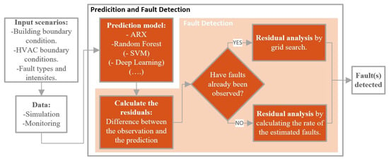
Figure 1.
Summary of FD procedure. The focus of this study is on the fault detection area highlighted in light red.
2. Description of Simulated Data and System Faults
The simulation was build upon an empirical validation experiment of Annex 58 and Annex 71. A detailed description of the two identical full-size buildings of the Fraunhofer Institute for Building Physics in Holzkirchen, Germany, and data can be found in [20,21,22,23,24].
The data set is obtained through detailed simulation with the building performance simulation (BPS) program IDA Indoor Climate and Energy (IDA ICE) [25]. IDA ICE is a multizone equation based simulation program to describe and simulate the behaviour of buildings and HVAC systems. A model of the building and HVAC system is physically described and simulated. The simulation uses the house description of Annex 58 and the climate boundary conditions of January and February 2019 in Holzkirchen [26] (Annex 71).
For the simulation model, each room was equipped with a 2000 W electric radiator with a longwave radiation fraction of . The heating set point of the air temperature was set to and controlled room wise by a thermostatic control with a dead band of K.
The simulation integrates an MHVR (Mechanical Ventilation with Heat Recovery) air handling unit with a heat recovery of 80 percent with an integrated MVHR summer bypass (possibility to switch off the heat recovery during summer months). Table 1 shows the setting of the MHVR for the different rooms, divided into rooms with supply air and return air. The living room and the kitchen have an open floor plan.

Table 1.
Air handling unit settings.
The simulation includes a simple occupancy plan of a four-person household with the absence of users between 7:30 and 17:00 each day. The occupancy is set as presented in Table 2.

Table 2.
Occupancy settings.
The data set starts on 1 January and ends 28 February. The first month (1–31 January), the building runs in regular operation. The second month (1–28 February) includes faults in the operation of the building. In this study, three faults are selected. The first fault (F1) is the tripping of the circuit breaker due to an overload of the upper floor power cable or due to a short circuit. The result is the loss of heating power on the upper floor. It is possible to deactivate the heat recovery of the ventilation system through a bypass to prevent overheating during the summer months. In the second fault (F2), the bypass disables during the heating period. This fault results in cold supply air temperatures in the ventilation system. In the third fault (F3), the room temperature thermostat of the living room is broken. The result is a changed setpoint temperature of 28 . Table 3 gives a detailed description of the faults and their start and end times.

Table 3.
Integrated system fault settings.
The data set contains the indoor and outdoor properties shown in Table 4. Air temperature for each room and total heating power supplied by all electrical radiators are measured indoors. The outdoor properties are the air temperature, relative humidity, diffuse and direct solar irradiation on horizontal surfaces, and wind speed and wind direction.

Table 4.
Simulated data properties.
3. Statistical Tests
The presented statistical tests are implemented with the programming language R [27], and the user interface RStudio [28]. The graphics were created with the R package “ggplot2” [29].
The predictive models for the response total heating power use as predictors the indoor temperatures of all rooms, all outdoor information, as listed in Table 4 and the daytime in hours. The estimated total heating power is the model output and the values of the total heating power one hour and two hours ago at each point in time are added as predictors (features) to the models.
The predictive modelling is carried out with the method random forest [30] and an ARX (autoregressive with exogenous variables) time series model [31]. To predict the total heating power in February, the January data is used to train a model. The total heating power in January is predicted with a 4-fold cross-validation. The 4-fold cross-validation divides the January data into four nearly equally sized parts. Then three of these parts predict the reminding part in order to evaluate the models. The difference between the real values (responses) and the predicted values of the total heating power are the residuals. Let be the response variable of the observed total heating power and the predicted total heating power from a model at the time . Then denotes the residual at the time t and the vector of the residuals. Furthermore is defined for a fixed .
Figure 2 shows the January and the February residuals for the developed random forest and the ARX model.
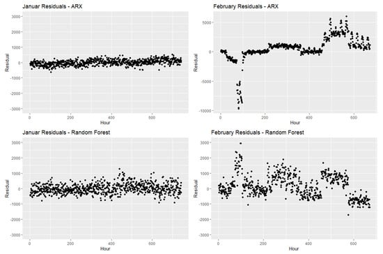
Figure 2.
January and February residuals for ARX model and random forest model.
After successful modelling, the typical properties of residuals are to be statistically tested. A fault in the data process is assumed if the behaviour of the residuals deviates significantly from the standard properties. The special properties of residuals depend on the modelling methodology, the data structure of the learning sample, as well as on the prediction quality of the model.
It is assumed that the residuals have a median of zero, are independent and therefore uncorrelated from each other, and behave randomly.
The Sign Test [32] and the Wilcoxon Signed-Rank Test [33] are suitable for testing for median equal to zero. The Turning Point Test [34] is well suited for testing independence, the Box-Pierce Test and the Ljung-Box Test [35] for autocorrelation. Randomness can be tested with the Bartels-Rank Test, Cox-Stuart Trend Test, Difference-Sign Test and Mann-Kendall Rank Test [36]. In total, this study examines the residuals using nine tests divided into four test objectives.
3.1. Moving p-Value
The moving residuals for the shift s with time window length , which represents the sample size of the moving residuals, are defined by The moving residuals are used in order to avoid testing all residuals at once. If is the p-value of the statistical test T, it is used , for a fixed L, to examine periods for faults. If the p-value of a test is less then a previously selected significance level , then the null hypothesis of this test is significantly not met [17], page 5 ff. For all nine tests the null hypothesis is that a certain property of the residuals is fulfilled. Therefore it applies that for each test a fault is suspected when the p-value of this test is smaller then .
3.2. Mean p-Value (MPV)
A disadvantage of the p-values of the moving residuals used so far is that it can be recognized at which shift s the p-value is no longer as expected, but not at which time point. In the following, a new constructed function determines faulty time points. This is made possible by a mean of the p-values from the moving residuals. Let (1) be the mean p-value, in future called MPV.
where denotes the indicator function with , if and 0 else. The MPV for a given test T and a window length L is for each the mean of all p-values generated by moving residuals that used in the calculation.
For the fault detection it applies, if , then the test T assumes a fault at time point t. The fault detection presented here uses a combination of tests, which raises the question of how many tests must assume at least one fault to assume a fault in total. This value is abbreviated with H. The value of H is at least one and at most the whole number of tests which are used in the analysis. In this work nine tests are used. Thus an automated fault detection can be defined by using the three parameters , and . Therefore, in the following each triple is simplified termed as a decision rule. For the application G is replaced by a large subset of G. Let (2) be the fault function.
Since there are no system faults implemented in the January data a limitation is made to the decision rules which erroneously detect faults. Accordingly, a decision rule from the following set (3) is required which is refereed to as choice set.
3.3. Parameter Optimization in the Case of Observed Faults
A grid search finds with the known time points of faults an optimized decision rule , which minimises a previously defined fault rate. This optimization shows on the data of this study good results. The applicability of the model, which was optimized by this procedure on another data, was not tested so far. A problem could be that the decision rule adapts to the data too individually. In future works, the procedure should be repeated with other validation data. Only when data with known faults is available, this technique can be used, which is why other procedures are presented below.
3.4. Parameter Optimization in the Case of Unobserved Faults
A realistic, application-oriented situation is that the system faults are unobserved. This study looks for a method to derive a valid decision rule from the choice set without prior knowledge of the faults. The aim is to find the decision rule from the choice set C, which recognizes the faults as good as possible. Note that there are many decision rules in the choice set that never assume a fault. A possible approach to get a decision rule with a high statistical power would be to restrict the choice set via the adjacency. If a decision rule in the choice set is adjacent to a decision rule that estimates exactly one fault in January, then this decision rule will correctly estimate January, and it should be able to classify faults with a high power. An example of such an adjacency can be seen in Figure 3, which is a simplified representation of two parameters. The figure shows the fault estimations of 25 decision rules.
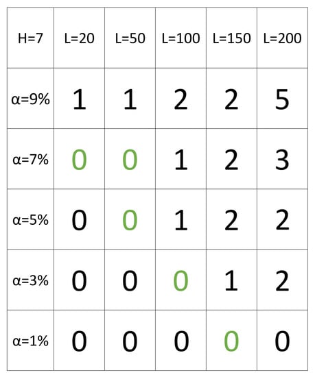
Figure 3.
Example for restricting C using adjacency, simplified for . In green are the combinations of C, which are adjacent to a combination which assumes exactly one fault.
A disadvantage of this approach is that it is likely to dispose of many good combinations. Moreover, in future works alternative measures of adjacency could be investigated.
Another way is to determine the most frequent characteristic of each component from the set C, i.e., the mode for each component. This means a search for the values defined in (4)–(6) is needed
where denotes the number of elements of a set A. Finally, it is checked whether and for this case is the selected decision rule. Instead of the mode, this procedure can also be performed with other measures of location such as mean or median. However, the choice quantity should be further restricted beforehand. This can be done by applying all decision rules to February and removing the decision rules that predict too few or too many times faults in the February data.
3.4.1. Rate of Estimated Faults
If no suitable element can be found directly from C with the previous methods, the following approach can also be pursued. For this, each element of the choice set must contain a decision at any time. Each decision rule can have two values per point in time, zero if it is not classified as fault and one if it is classified as a fault. The number of decision rules that classify for faults are formed by the sum of the decisions for each element from C (at any time). Next, these values are divided by the number of decision rules that classify for faults at least once in February. This way, the decision rules that never classify a fault are ignored. This rate is referred to as the rate of estimated faults. If this rate is greater than a fixed threshold value, a fault is assumed. The following Table 5 serves as a simplified example.

Table 5.
Example for the calculation of the rate of estimated faults. The number of decision rules that assume a fault is marked in blue.
Table 5 shows that there are four time-points considered, and C contains five decision rules. Two of these five decision rules never assume a fault. Therefore, the sum of the dichotomous decision rule values per time is divided by three (blue in Table 5). The threshold value chosen here is 1/2 so that for the time points two and three faults are classified.
3.4.2. Restricting Areas
The previous methods were based on the MPV, which was used to estimate the exact times when faults accrue. However, if it is sufficient to limit the faults to certain periods, the following steps can be taken. First, a significance level , e.g., is determined. Then the p-values of all January residuals of each test are calculated, and the tests with a p-value smaller than are discarded. The remaining tests are now applied to the February residuals and the tests with a p-value greater than are discarded. The tests that remain reject the null hypothesis in February but not in January. Step by step, the range of faults is limited by dividing the February residuals into the first and the second half. The p-values of both halves are calculated. Each half with a p-value greater than is further divided, and the process can be repeated. If there are only p-values bigger than in a range, it can be assumed that there is no fault in this range. However, the problem with this procedure is that p-values strongly depend on the sample size. Therefore the threshold needs to be gradually adapted depending on the sample size.
4. Results
4.1. The Case of Observed Faults
This research uses the decision rules of the choice set for each data set and each model with the lowest prediction error rate. This study analysed whether the residual analysis delivers better results when the first, the second or the third fault or all three faults are in the data. Figure 4 shows the representation of the optimal decision rule for both prediction models when only the first of the three faults, see Table 3, are present in the data.
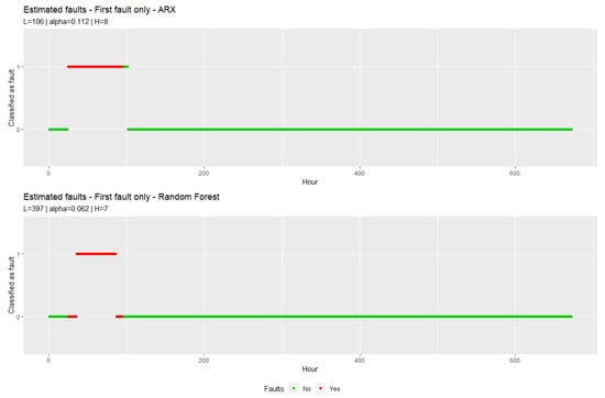
Figure 4.
Fault estimate with decision rule for the ARX model and for the random forest model. The periods with faults in the data are marked in red. The y-axis indicates if the decision rule decided on faults.
When adding only the second fault to the data, it yields to the following Figure 5 with the same procedure.
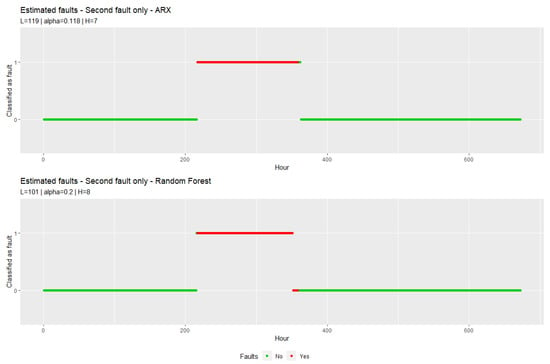
Figure 5.
Fault estimation with decision rule for the ARX model and for the random forest model. The periods with faults in the data are marked in red. The y-axis indicates if the decision rule decided on faults.
Figure 6 and Figure 7 show the cases where only the third respectively all faults are present in the data.
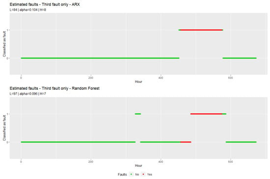
Figure 6.
Fault estimation with decision rule for the ARX model and for the random forest model. The periods with faults in the data are marked in red. The y-axis indicates whether the decision rule decided on faults.
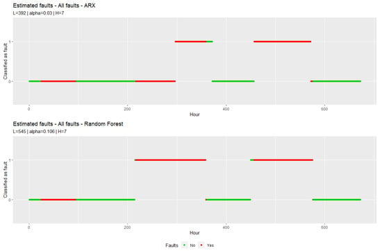
Figure 7.
Fault estimate with decision rule for the ARX model and for the random forest model. The periods with faults in the data are marked in red. The y-axis indicates whether the decision rule decided on faults.
The chosen procedure to test the residuals properties can detect the faults in HVAC systems. The graphical evaluation provides that if there is a fault in the data set, the faults are detected well or very well. When analysing the data set containing all three faults, the first fault is not detected. The optimal decision rule for the chosen prediction models differ from (84, 10.4%, 8) to (545, 10.6%, 7). The decision rules used are all different and far apart, so it is difficult to choose one decision rule for all cases.
4.2. The Case of Unobserved Faults
An effort was made to find the best decision rule for the case of unobserved faults. These two variations of the decision rule that detect faults were explored: a method that limits the choices through adjacency and a method that involves the change of the mode. The first method rejected too many good decision rules, while the second method got influenced by the decision rules, that never contain estimated faults. Additionally the change of the mode did not improve the decision rules. The method of restricting areas did not lead to any results. All three methods were rejected and instead the rate of estimated fault was analysed. If the faults are detected with no prior knowledge of the exact time points and without empirical values for a decision rule, then the faults can be predicted by calculation of the rate of estimated faults. The following shows the result for the data sets with three different faults and a data set with no faults for the chosen prediction models. Figure 8 shows the results for the first fault, Figure 9 the second fault, and Figure 10 the third fault.
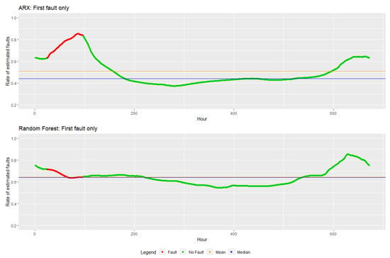
Figure 8.
Rate of estimated faults for the first fault. In red, the period with fault, in green the period without fault, in blue is the median, and the mean of the estimated rates is in orange.
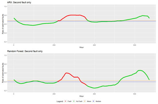
Figure 9.
Rate of estimated faults for the second fault. In red, the period with fault, in green the period without fault, in blue is the median, and the mean of the estimated rates is in orange.
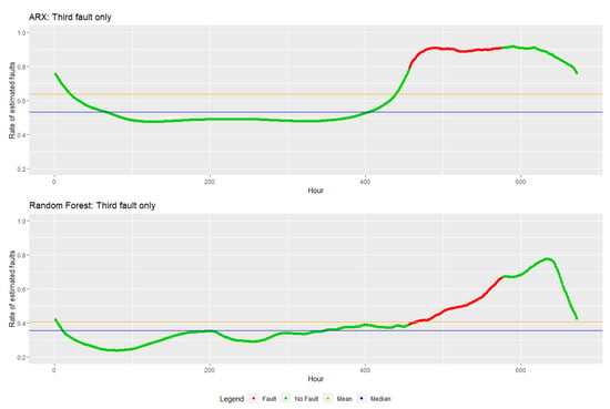
Figure 10.
Rate of estimated faults for the third fault. In red, the period with fault, in green the period without fault, in blue is the median, and the mean of the estimated rates is in orange.
In Figure 11, you can see the rate of estimated faults when the data set implements all three faults.
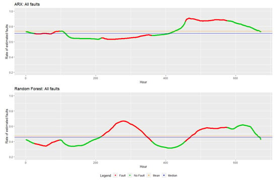
Figure 11.
Rate of estimated faults with all faults. In red, the period with fault, in green the period without fault, in blue is the median, and the mean of the estimated rates is in orange.
When evaluating the faultless data, one gets the representation in Figure 12.
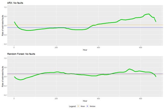
Figure 12.
Rate of estimated faults for the faultless data. In red, the period with fault, in green the period without fault, in blue is the median, and the mean of the estimated rates is in orange.
The fault detection is carried out via a threshold value. This study uses the median and the mean of estimated rates (shown in orange and blue in the figures). The difficulty is to define the appropriate threshold value between zero and one. The Figure 8, Figure 9, Figure 10, Figure 11 and Figure 12 show the course of the rate of estimated faults and the selected threshold values. The graphical evaluation shows that faults are detected but that many areas are also incorrectly identified as faults. It seems that both the median and the mean of estimated faults are too low thresholds. Especially the fault detection from 600 h shows a fault graphically if there is no fault.
4.3. Comparison Prediction Models
The January residuals, created by a 4 fold cross-validation, are useful to compare both prediction models. This can be done by using the mean squared error (MSE) of each model, which is defined by . For the ARX model, the calculated MSE equals 31,001.55, and for the random forest, it is . For this reason, the ARX model seems to be a better choice to predict the total heating power. Usually the hyperparameters of the random forest should be optimized to reduce the MSE but in this case the recommended values by Leo Breimann [15] were just used to perform the fault detection. In this way one tests how the fault detection methods perform for residuals with high variance. For the observed case Figure 4, Figure 5 and Figure 6 show the results when only adding one fault to the data. The decision rule using the ARX model delivers better results because the decision rule based on the random forest model often suspects faults where no faults are and match the existing fault less accurately. If all faults are in the data as shown in Figure 7, both models detect the third fault very well, the ARX model has problems with the second fault, and both models recognise the first fault not well. In the case of unobserved faults, the ARX detects the fault better if there is only one fault in the data set. For more faults in the data set, the random forest worked better. The MSE of both the ARX and the random forest models seem not to substantially affect the detection of faults based on the residual analysis.
5. Conclusions
This study uses residual analysis for fault detection of HVAC systems in buildings. A detailed simulation of a residential case study house provided the data for the analysis. The predictive modelling of the total heating power was carried out with the method random forest and ARX (autoregressive with exogenous variables) time series model. The fault detection was carried out by a residual analysis. The residuals were calculated directly from the predictions. A combination of statistical tests explored the white noise properties of the residuals, while a data-driven decision rule that combines multiple tests predicted the faults. The methods for fault detection developed in this study could replace a graphical, user-subjective evaluation of a residual plot using an automatic, data-based approach.
The fault detection method that uses residual analysis has several advantages: For one the method does not depend on the prediction model applied, furthermore information such as model parameter estimations and specific model structures are become superfluous. The research has proved that the methods of fault detection can be applied and different types of prediction models such as time series models and procedures of machine learning (including black-box methods) are suitable. Statistical tests can be added or removed depending on the suspected residual properties.
This study introduces two different methods of residual analysis one that finds a decision rule by grid search when faults are observed and the other that uses the rate of estimated faults when faults are unobserved. Better results are achieved with the case of observed faults then with the case of unobserved faults. Both fault detection methods depend heavily on the p-values, which usually depend on the sample size, and the methods had to be consistently adjusted to the specific situation and the given sample size.
The results show that the method for the case of unobserved faults should be pursued further in the future. Since in practice the faults will not be observed. The evaluation of the case of unobserved faults has brought with it the following difficulty: The results of the method on unobserved faults show that the threshold value is difficult to find. The threshold value determines how accurate a fault is predicted and has the function of a trade-off between specificity and sensitivity of the classification rule. Fault detection based on the rate of estimated faults can be used without prior knowledge of the faults. Additionally, this procedure also finds faults when none are present, see Figure 12. However, the advantage of this method, which is to ignore the decision rule that never detect faults, in this case becomes a disadvantage. By adjusting the threshold for the decision on faults, the ratio between the decision rules that identify at least one fault and the decision rules overall in the choice set could be improved. At the end of the test month (approx. 600 h), the FD method detects a fault where there is no fault. We interpret this to be the case that the seasonal temperature fluctuations were not sufficiently represented in the training data set, and the temperature increase during this period (winter-spring transition) was therefore detected as a fault.
The method invites the application on data measured on-site. A real building evaluation could be performed using a learning data set based on a building simulation (with simulated, observed faults) of the same building. Consequently, it is essential to test the applicability of a decision rule based on simulated building data on the behaviour of the original building. The accuracy of the building simulation would then be a significant factor in the successful application of the method.
6. Outlook
In the next stage of this study, we plan to apply more statistical methods for fault detection on the one hand and the other hand, an extended dataset to represent seasonal fluctuations better. We also plan to increase the number of technical faults in the ventilation system, in the heating and control system and a hydraulic problem. In a third phase of our study we plan to apply the developed fault detection models based on the simulated annual data set to data measured in situ.
The following methods could be suitable for finding an optimal algorithm to determine the best decision technique: defining upper and lower bounds for residuals, using the coefficient of determination, and the correlation comparison of the sensors.
A first new approach is to derive an upper and a lower bound using the residuals in the fault-free state. Then a fault might exist if residuals in a row are outside of the bound.
Mattera et al. [11] present a second model approach which we plan to investigate as well. The coefficient of determination () between the predicted value and the observed value per day is used to predict faults. In linear regression, a value of the coefficient of determination of one indicates a perfect linear relationship, while a coefficient of determination of zero indicates no linear relationship. Matera et al. assume a fault if is low. Instead of the coefficient of determination, other measures like the mean squared error would also be possible indicator for the presence of faults. Matera et al. also suggested using each sensor as a response to determine the specific cause of the fault. In future studies statistical methods to estimate (in an automated and data-driven way) the cause of a fault can be considered.
In addition to a residual analysis based on a predictive model of one response, other approaches are also conceivable. An idea for such an approach is an overall correlation comparison, which is conducted by calculating the correlation (with respect to the linear or monotone relationships) between all sensors per day. Then, with the help of the fault-free state, an upper and a lower bound is defined for each sensor pair. If a certain number of correlations is outside the bound, a fault can be assumed. The advantage of this method is that it would allow us to determine, without much additional effort, which sensors are suitable to detect the fault by taking into consideration not only the number of correlations outside the boundary but also which pairs are outside the boundary.
Creating a whole network of prediction models for real sensors as the response variables could be a useful extension of an overall correlation comparison. The predicted values as virtual sensors are checked against the observed values of the real sensors. The basis for the development of decision rules for fault detection could then be the deviation between the behaviour of the whole prediction network on faultless data and the behaviour of the network on a data set with faults.
Author Contributions
Conceptualization, M.P., L.H., F.S., U.S., U.W. and M.W.; Data curation, M.P., F.S. and M.W.; Formal analysis, M.P.; Funding acquisition, U.S. and U.W.; Investigation, M.P., L.H., F.S., U.S. and U.W.; Methodology, M.P. and U.W.; Project administration, L.H., U.S. and U.W.; Software, M.P.; Supervision, U.S. and U.W.; Validation, M.P.; Visualization, M.P., F.S. and M.W.; Writing—original draft, M.P., L.H. and U.W.; Writing—review & editing, L.H., U.S., U.W. and M.W. All authors have read and agreed to the published version of the manuscript.
Funding
Supported by: Federal Ministry for Economic Affairs and Energy on the basis of a decision by the German Bundestag. FKZ:03ET1509C.
Conflicts of Interest
The authors declare no conflict of interest.
Abbreviations
The following abbreviations are used in this manuscript:
| AFDD | Automated fault detection and diagnostics |
| ARX | Autoregressive with exogenous variables |
| C | Choice set |
| FD | Fault detection |
| FDD | Fault detection and diagnostics |
| Coefficient of determination | |
| Decision rule | |
| ECB | Energy in Buildings and Communities Programm |
| Estimated total heating power | |
| Fault function | |
| H | Minimum number of MPV that have to assume a fault before in total a fault is assumed |
| HVAC | Heating, Ventilation and Air Conditioning |
| Indicator function | |
| IEA | International Energy Agency |
| MPV, | Mean p-value |
| MSE | Mean squared error |
| , and | Mode of L, , H |
| Moving residuals | |
| n | Number of observations |
| Observed total heating power | |
| p-value of the statistical test T | |
| Residual at time t | |
| G | Set of decision rules |
| Significance level | |
| t | Time |
| L | Time window length |
| Vector of residuals | |
References
- BMWi. Energieeffizienzstrategie Gebäude. Wege zu Einem Nahezu Klimaneutralen Gebäudebestand; Bundesministerium für Wirtschaft und Energie (BMWi) Öffentlichkeitsarbeit. Available online: www.bmwi.de (accessed on 11 August 2019).
- Mills, E. Building commissioning: A golden opportunity for reducing energy costs and greenhouse gas emissions in the United States. Energy Effic. 2011, 4, 145–173. [Google Scholar] [CrossRef]
- Dexter, A.; Pakanen, J. Conservation in Buildings and Community Systems—Technical Synthesis Report Annex 34; Technical Report; International Energy Agency: Paris, France, 2006. [Google Scholar]
- Lin, G.; Kramer, H.; Granderson, J. Building fault detection and diagnostics: Achieved savings, and methods to evaluate algorithm performance. Build. Environ. 2020, 168, 106505. [Google Scholar] [CrossRef]
- Mondal, B. Artificial Intelligence: State of the Art. In Recent Trends and Advances in Artificial Intelligence and Internet of Things; Balas, V.E., Kumar, R., Srivastava, R., Eds.; Springer: Cham, Switzerland, 2020; Volume 172, pp. 389–425. [Google Scholar] [CrossRef]
- Yan, K.; Shen, W.; Mulumba, T.; Afshari, A. ARX model based fault detection and diagnosis for chillers using support vector machines. Energy Build. 2014, 81, 287–295. [Google Scholar] [CrossRef]
- Luo, B.; Wang, H.; Liu, H.; Li, B.; Peng, F. Early Fault Detection of Machine Tools Based on Deep Learning and Dynamic Identification. IEEE Trans. Ind. Electron. 2019, 66, 509–518. [Google Scholar] [CrossRef]
- Kim, W.; Katipamula, S. A review of fault detection and diagnostics methods for building systems. Sci. Technol. Built Environ. 2018, 24, 3–21. [Google Scholar] [CrossRef]
- Lo, N.G.; Flaus, J.M.; Adrot, O. Review of Machine Learning Approaches In Fault Diagnosis applied to IoT System. In Proceedings of the International Conference on Control, Automation and Diagnosis (ICCAD’19), Grenoble, France, 2–4 July 2019. [Google Scholar]
- Ge, Z.; Song, Z.; Ding, S.X.; Huang, B. Data Mining and Analytics in the Process Industry: The Role of Machine Learning. IEEE Access 2017, 5, 20590–20616. [Google Scholar] [CrossRef]
- Mattera, C.; Quevedo, J.; Escobet, T.; Shaker, H.R.; Jradi, M. A Method for Fault Detection and Diagnostics in Ventilation Units Using Virtual Sensors. Sensors 2018, 18, 3931. [Google Scholar] [CrossRef] [PubMed]
- IEA ECB Annex 71. Building Energy Performance Assessment Based on In-Situ Measurements. 2016–2021. Available online: https://www.ecbcs.org/projects/project?AnnexID=71 (accessed on 15 November 2019).
- IEA ECB Annex 58. Reliable Building Energy Performance Characterisation Based on Full Scale Dynamic Measurements. 2011–2016. Available online: https://www.iea-ebc.org/projects/project?AnnexID=58 (accessed on 15 November 2019).
- Parzinger, M.; Hanfstaengl, L.; Sigg, F.; Wirnsberger, M.; Wellisch, U.; Spindler, U. Identifying faults in the building system based on model prediction and residuum analysis. E3S Web Conf. 2020, 172, 22001. [Google Scholar] [CrossRef]
- Breiman, L. Random Forests. Mach. Learn. 2001, 45, 5–32. [Google Scholar] [CrossRef]
- Madsen, H. Time Series Analysis; Texts in Statistical Science, 72; Chapman and Hall/CRC: Boca Raton, FL, USA, 2008. [Google Scholar]
- Pruscha, H. Statistisches Methodenbuch: Verfahren, Fallstudien, Programmcodes; Springer: Berlin/Heidelberg, Germany, 2006. [Google Scholar]
- Box, G.E.P.; Jenkins, G.M.; Reinsel, G.C. Time Series Analysis; Forecasting and Control, 3rd ed.; Prentice Hall: Englewood Cliff, NJ, USA, 1994. [Google Scholar]
- Fassois, S.D.; Sakellariou, J.S. Time-series methods for fault detection and identification in vibrating structures. Philos. Trans. Ser. A Math. Phys. Eng. Sci. 2007, 365, 411–448. [Google Scholar] [CrossRef] [PubMed]
- Strachan, P.; Svehla, K.; Heusler, I.; Kersken, M. Whole model empirical validation on a full-scale building. J. Build. Perform. Simul. 2015, 9, 331–350. [Google Scholar] [CrossRef]
- Kersken, M.; Heusler, I.; Strachan, P. Erstellung eines neuen, messdatengestützten Validierungsszenarios für Gebäudesimulationsprogramme. In Proceedings of the Fifth German-Austrian IBPSA Conference, RWTH Aachen University, Aachen, Germany, 22–24 September 2014; pp. 144–151. [Google Scholar]
- Strachan, P. Twin Houses Empirical Dataset: Experiment 1; University of Strathclyde: Glasgow, UK, 2015. [Google Scholar] [CrossRef]
- Strachan, P. Twin Houses Empirical Validation Dataset: Experiment 2; University of Strathclyde: Glasgow, UK, 29 February 2016. [Google Scholar] [CrossRef]
- Kersken, M.; Strachan, P. Twin House Experiment IEA EBC Annex 71 Validation of Building Energy Simulation Tools—Specifications and Dataset, Version: 2020-05-20 11:00:07.0; IBP Fraunhofer-Institut für Bauphysik: Holzkirchen, Germany, 2020. [Google Scholar] [CrossRef]
- IDA Indoor Climate and Energy (IDA ICE), Simulation Tool. 2019. Available online: https://www.equa.se/en/ida-ice (accessed on 29 April 2020).
- Fraunhofer Institute for Building Physics IBP. 2019. Available online: https://www.ibp.fraunhofer.de/en.html (accessed on 29 April 2020).
- R Version 3.6.1 (Action of the Toes). Available online: https://www.r-project.org/ (accessed on 29 April 2020).
- RStudio Team. RStudio: Integrated Development Environment for R; RStudio, Inc.: Boston, MA, USA, 2019. [Google Scholar]
- Wickham, H. ggplot2: Elegant Graphics for Data Analysis; Springer: New York, NY, USA, 2016. [Google Scholar]
- Wright, M.N.; Ziegler, A. ranger: A Fast Implementation of Random Forests for High Dimensional Data in C++ and R. J. Stat. Softw. 2017, 77, 1–17. [Google Scholar] [CrossRef]
- Ohtsu, K.; Peng, H.; Kitagawa, G. Time Series Modeling for Analysis and Control; Springer: Berlin/Heidelberg, Germany, 2015. [Google Scholar]
- Arnholt, A.T.; Evans, B. BSDA: Basic Statistics and Data Analysis. 2017. Available online: http://CRAN.R-project.org/package=BSDA (accessed on 15 November 2019).
- Wilcoxon Rank Sum and Signed Rank Tests. Available online: https://stat.ethz.ch/R-manual/R-devel/library/stats/html/wilcox.test.html (accessed on 15 November 2019).
- Hart, A.; Martínez, S. spgs: Statistical Patterns in Genomic Sequences. 2018. Available online: http://CRAN.R-project.org/package=spgs (accessed on 15 November 2019).
- Box Pierce and Ljung Box Tests. Available online: https://stat.ethz.ch/R-manual/R-patched/library/stats/html/box.test.html (accessed on 15 November 2019).
- Caeiro, F.; Mateus, A. Randtests: Testing Randomness in R. 2014. Available online: http://CRAN.R-project.org/package=randtests (accessed on 15 November 2019).
© 2020 by the authors. Licensee MDPI, Basel, Switzerland. This article is an open access article distributed under the terms and conditions of the Creative Commons Attribution (CC BY) license (http://creativecommons.org/licenses/by/4.0/).