Towards Characterization of Indoor Environment in Smart Buildings: Modelling PMV Index Using Neural Network with One Hidden Layer


Abstract
:1. Introduction
1.1. The Novelty and Purpose of the Work
1.2. The Structure of the Paper
2. Materials and Methods
2.1. Personalized Thermal Comfort Models
The Present Research Gap, Literature Review
2.2. Classic PMV Thermal Comfort Evaluation Model
2.3. Deep Learning or Classic Network Structure
2.4. Data Processing, Network Structure, General Equation, Structure Identification Method
2.4.1. Data Processing—The Mapminmax Method
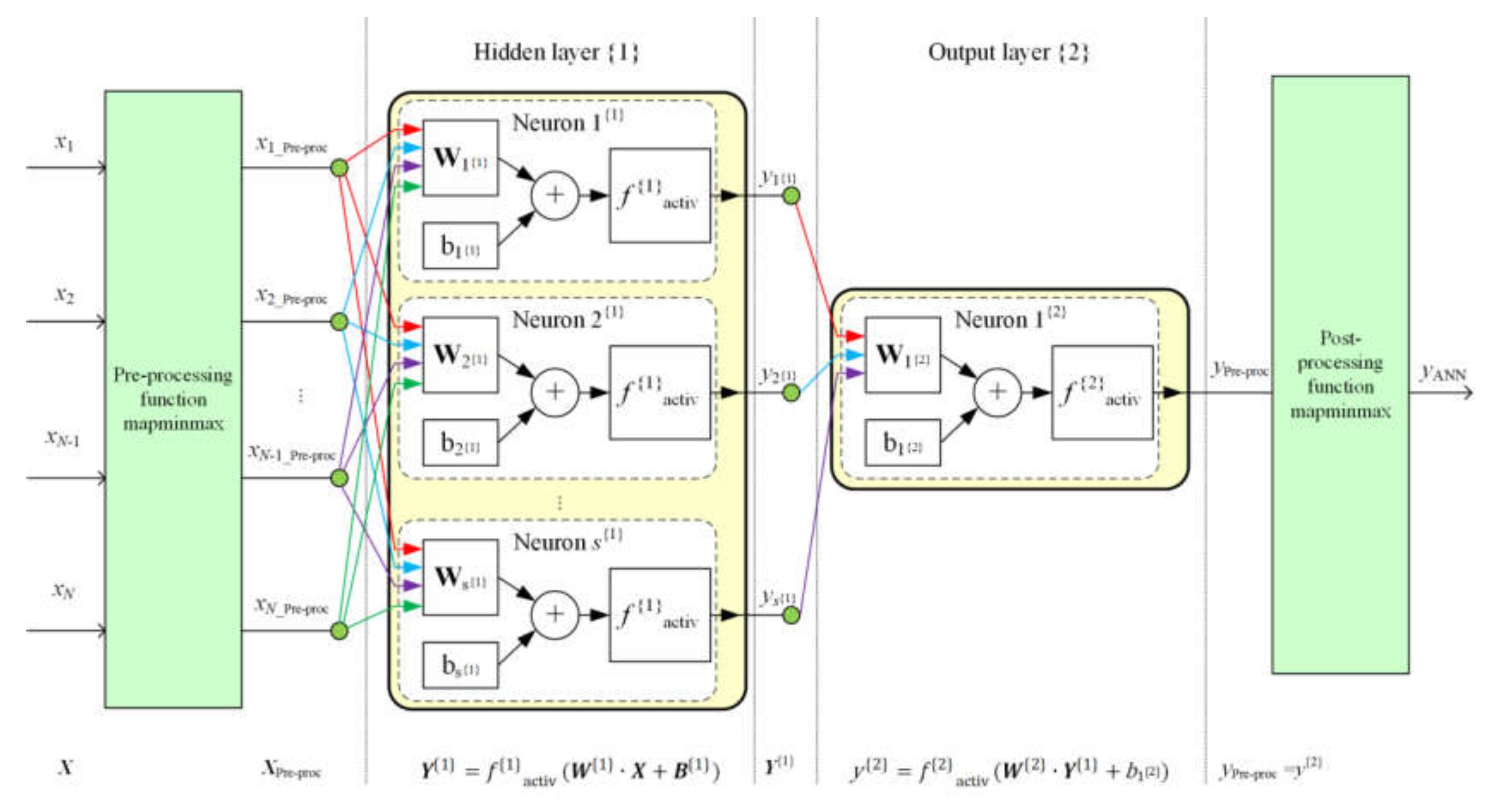
2.4.2. The Network Structure and its General Equation
- —data preprocessing operation,
- —data postprocessing operation,
- —input data vector,
- —matrix of weights of input arguments for the hidden layer,
- —column vector of biases for the hidden layer,
- —number of neurons in a hidden layer,
- —hidden layer activation function,
- —argument of the hidden layer transfer function, described as:
- —vector of weights of input arguments for the output layer,
- —bias for the output layer,
- —output layer activation function,
- —argument of the output layer transfer function, described as:
- —output value of the NN.
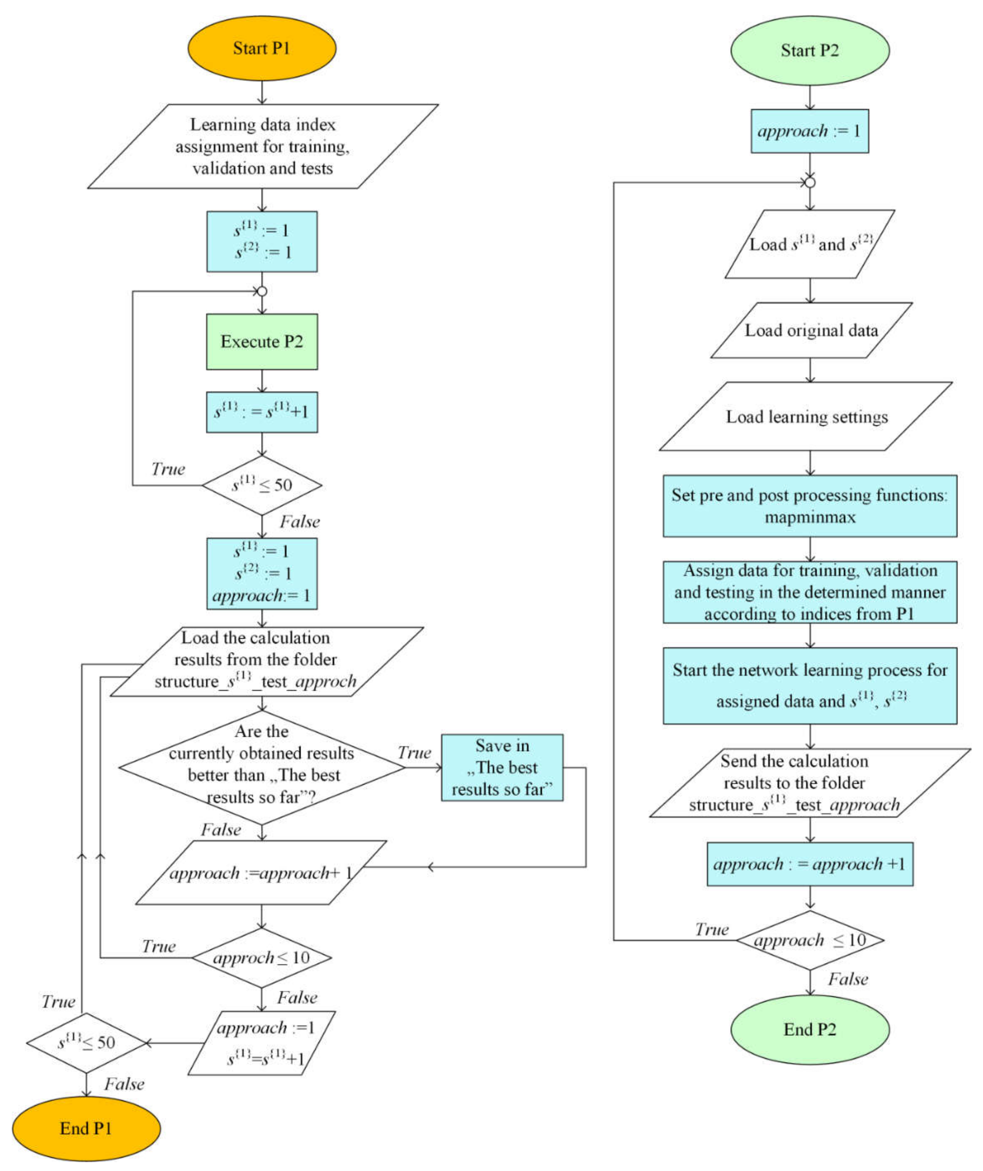
2.4.3. The Method Identifying Structures with the Best Number of Neurons in a Hidden Layer and the Best Neural Network
- —main criterion for choosing the best neural network structure,
- —number of neurons in the hidden layer,
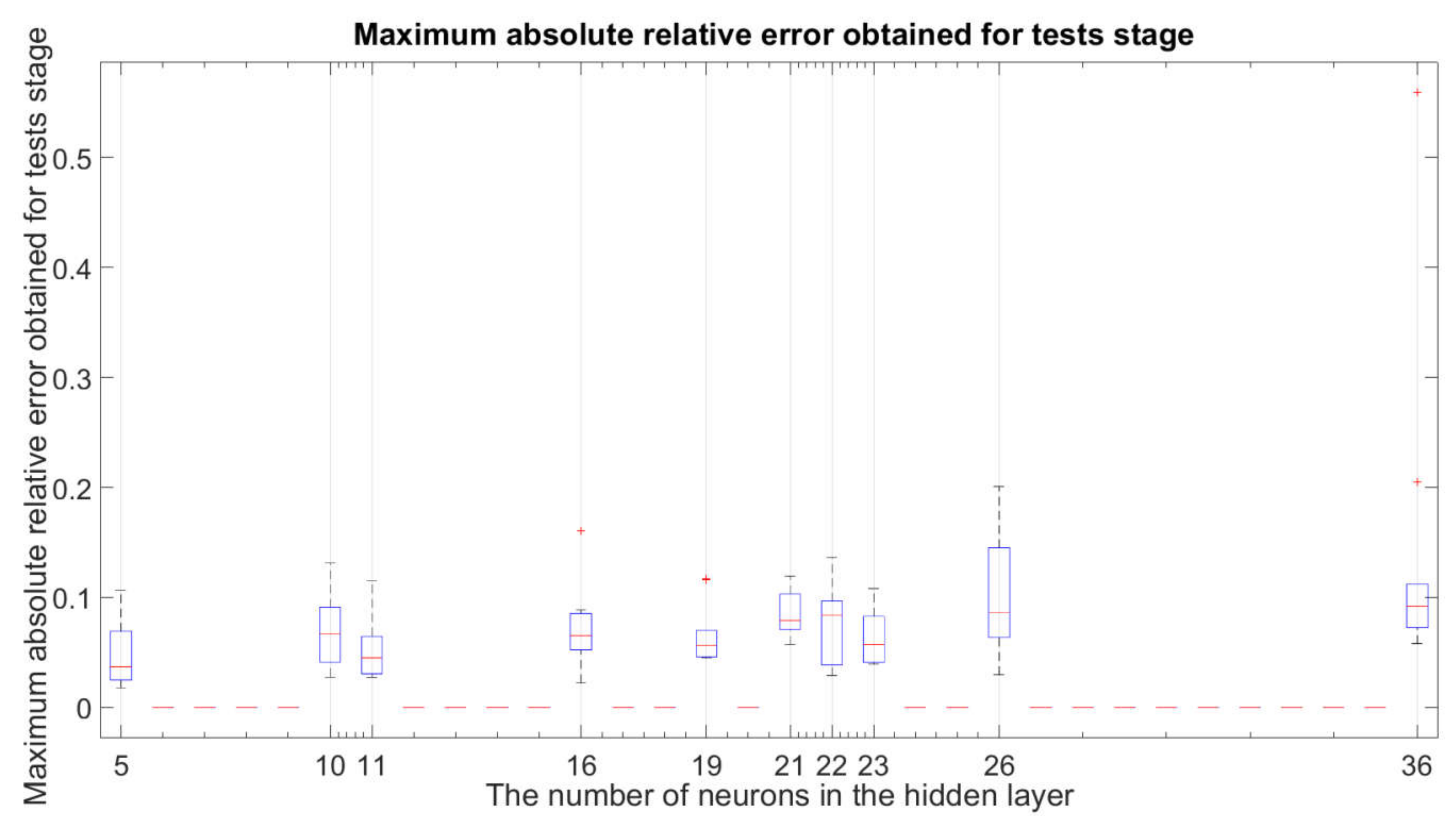
- —Maximum Absolute Relative Error obtained for the testing stage:where:
- —target for the network in testing stage,
- —output for the network in testing stage.
- —main criterion for choosing the best neural network structure,
- —the smallest number of neurons in the hidden layer,
- —maximum absolute relative error obtained for the testing stage.
- show robustness to changes of initial values of weights and bias in network neurons,
- are characterized by negligible impact of overfitting or underfitting.
2.5. Data for NN and Chosen Learning Specification
2.5.1. Data for NN
- general,
- environment,
- personal characteristics,
- comfort/productivity/satisfaction,
- behaviour,
- personal values,
- model.
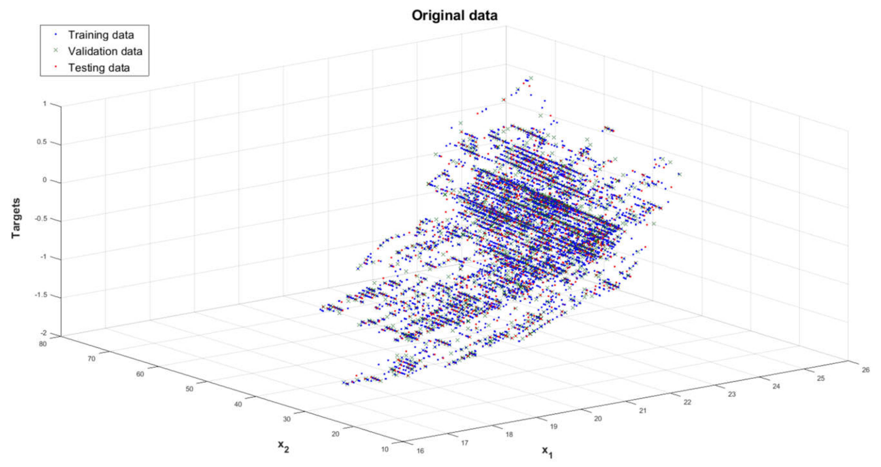
- matrix (inputs) with dimensions of 10,646 × 20, which is a series of input sets of samples assigned to the network learning process,
- the matrix Y (targets) with dimensions of 10,646 × 1, which is a series of PMV index reference output values obtained from the data included in the matrix X.
2.5.2. Chosen Learning Specification
- —number of sets for each learning stage: training , validation , tests ,
- —target for the network-reference PMV index value,
- —output of the network respective to the i-th target, which corresponds to estimated PMV index value.
2.6. Assessment of the Applicability of the Network Structure
2.6.1. Robustness Study Methodology
- less than 1, then one should use the indicator that contains the Sum of Absolute Errors made by the network;
- less than 10, then one should select the indicator that contains the average of the Sum of Absolute Errors made by the network. In this case, it is recommended to check how the structure behaves in terms of the selected indicator from the case ;
- greater than 10, then one needs to choose an indicator that amplifies network Errors by using the exponentiation operation.
2.6.2. Methodology of Overfitting and Underfitting Study
3. Results
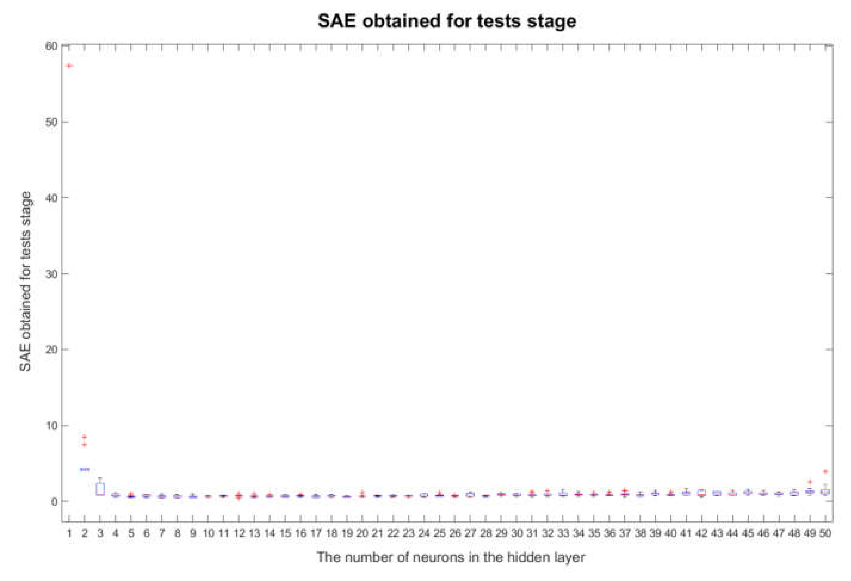
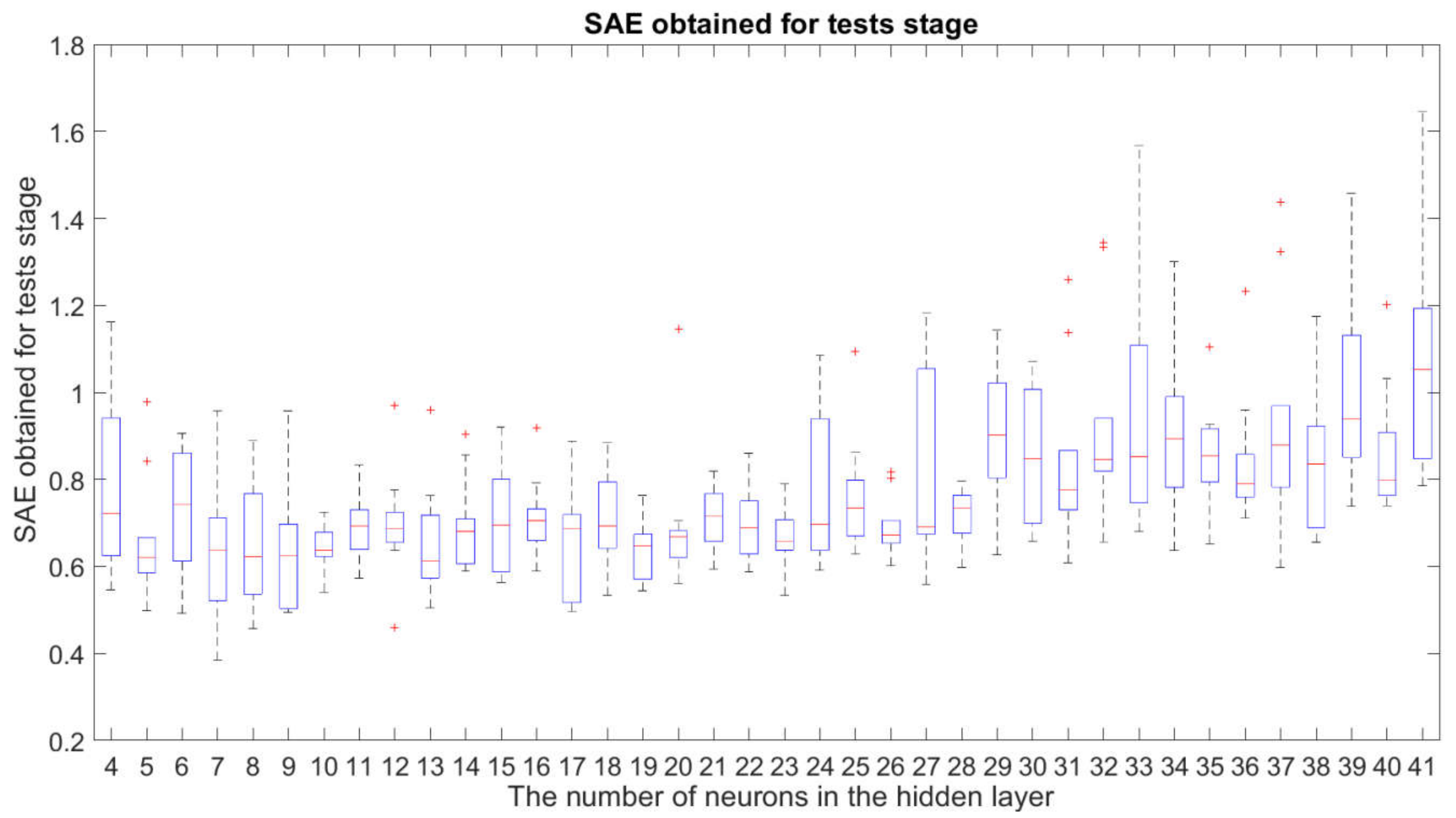
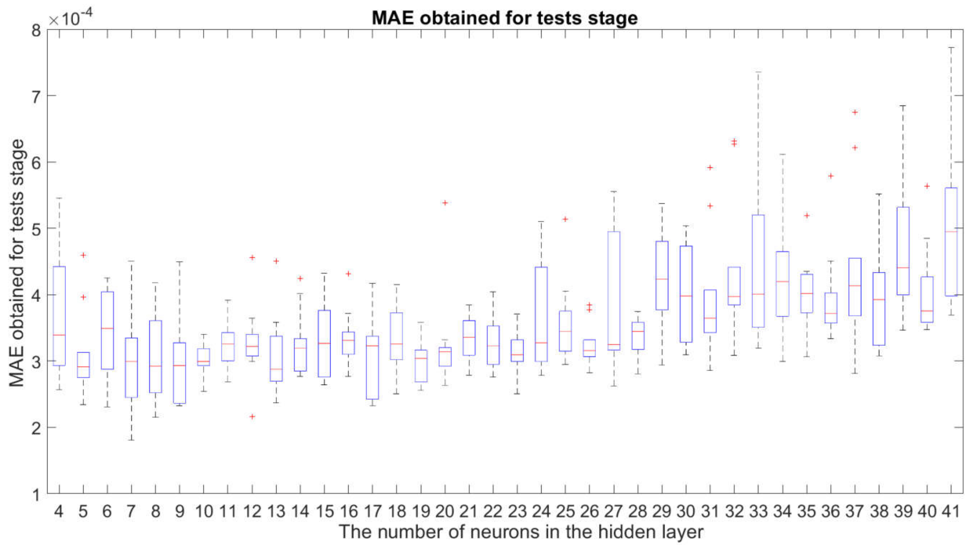
3.1. Robustness Study of the Examined Neural Network Structures
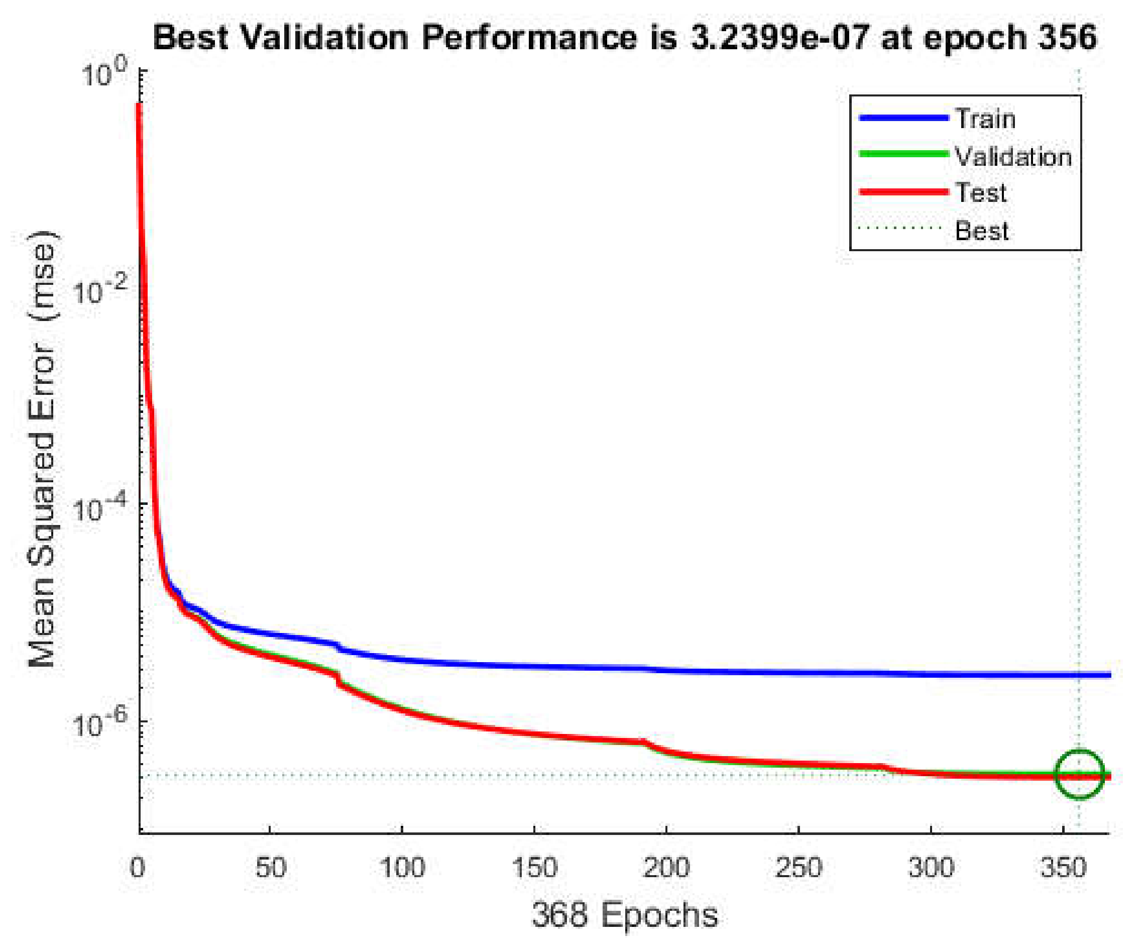
3.2. Study of Overfitting and Underfitting of the Examined Neural Network Structures
3.3. Identification of the Best Network Structure and the Best
- the fact described in Section 3.1 that the structures with are sufficiently insensitive to changes in the initial weights and bias of the neural networks for the network training stage;
- the fact described in Section 3.2 that the impact of underfitting or overfitting is acceptable or has negligible significance in the case of the structure for .
The Best Identified Neural Network and PMV Index Mathematical Model
- the dimensions of the matrix are specified; therefore, this information was noted in their subscripts;
- the elements of the matrix are identified numerical values.
4. Discussion
5. Conclusions and Future Research Program
- The method presented in the article enables filling the gap identified by the scientific community in comfort studies related to energy consumption in buildings.
- There are two approaches to filling the identified gap in the case of NNs with one hidden layer (Section 2.4.3): the first for the best quality fit of the model (Equation (5)), and the second one takes into account the quality of the fit with the minimum complexity of the NN model (Equation (7)).
- When designing the PMV index using NNs with one hidden layer, it is necessary to perform a robustness study (Section 3.1.) along with an overfitting and underfitting study (Section 3.2). Otherwise, there is a high likelihood (in the analyzed case about 80%) that NN will not be usable.
- NNs with one hidden layer enable PMV index modelling with almost perfect quality of model fit as long as the best structure identification method is used (Section 2.4.3 and Section 2.6).
- The use of the identification method (Section 2.4.3 and Section 2.6) compared to similar studies with NNs with one hidden layer gave better results in each case.
- The method presented in the article (Section 2.4.3 and Section 2.6) makes it possible to formulate the equation (Equations (20) and (A1)) characterizing individual thermal comfort for the object under study in terms of its basic functionality.
Funding
Acknowledgments
Conflicts of Interest
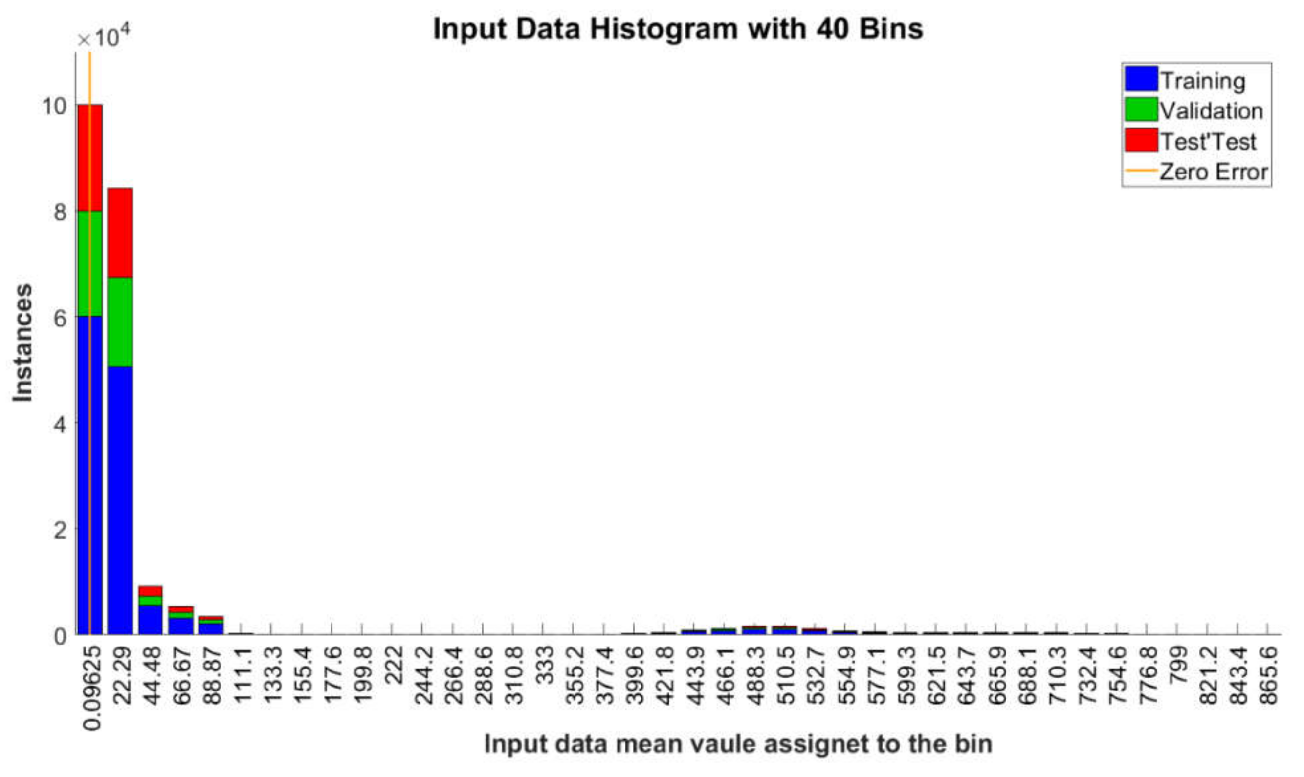
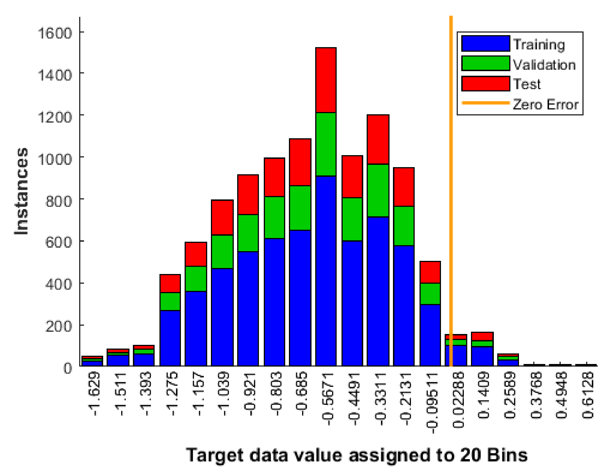
Appendix A. The Histogram of All Input Data and Reference Output Values (Targets) Assigned to the Learning Process with the Division into Learning Stages
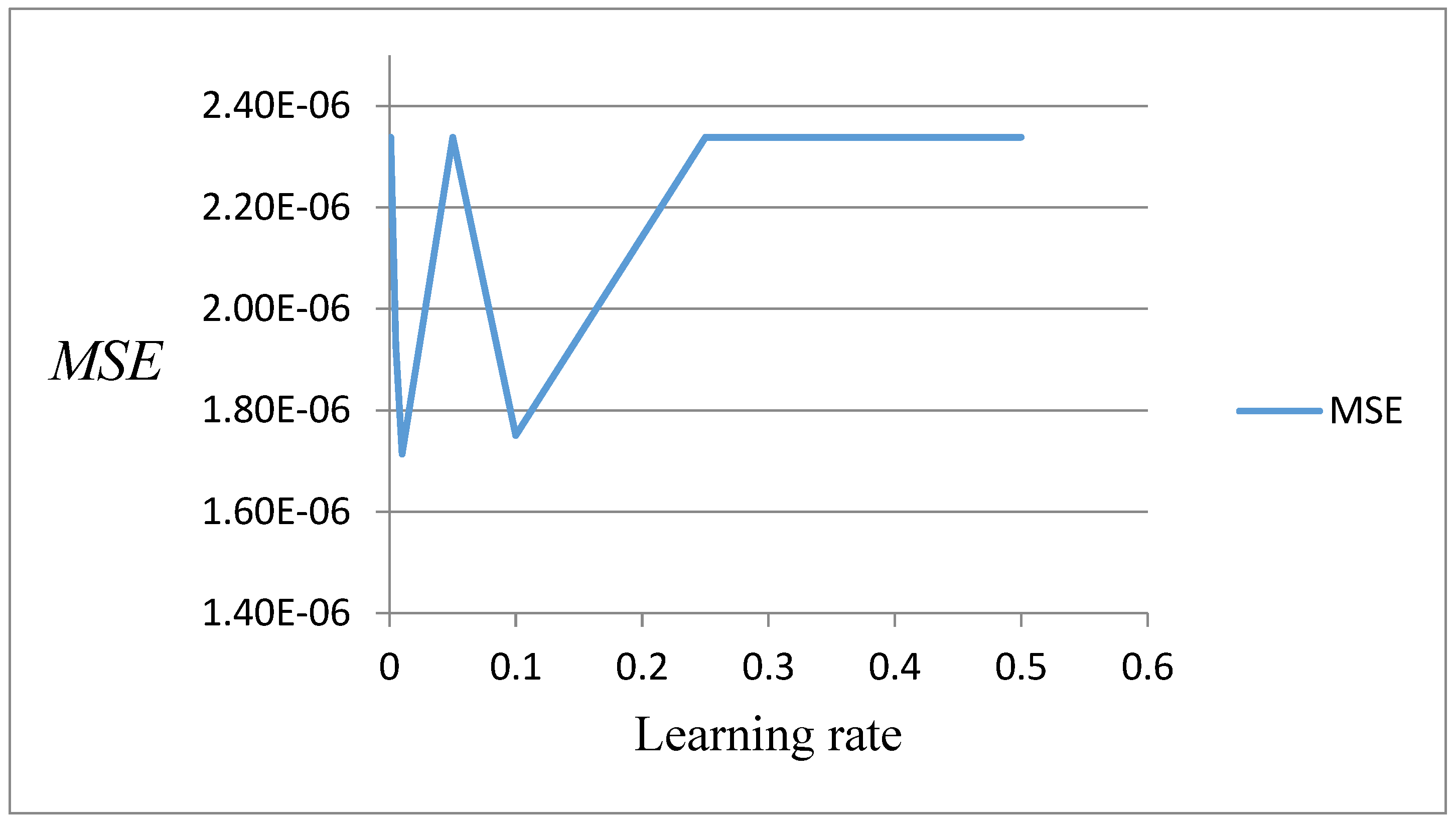
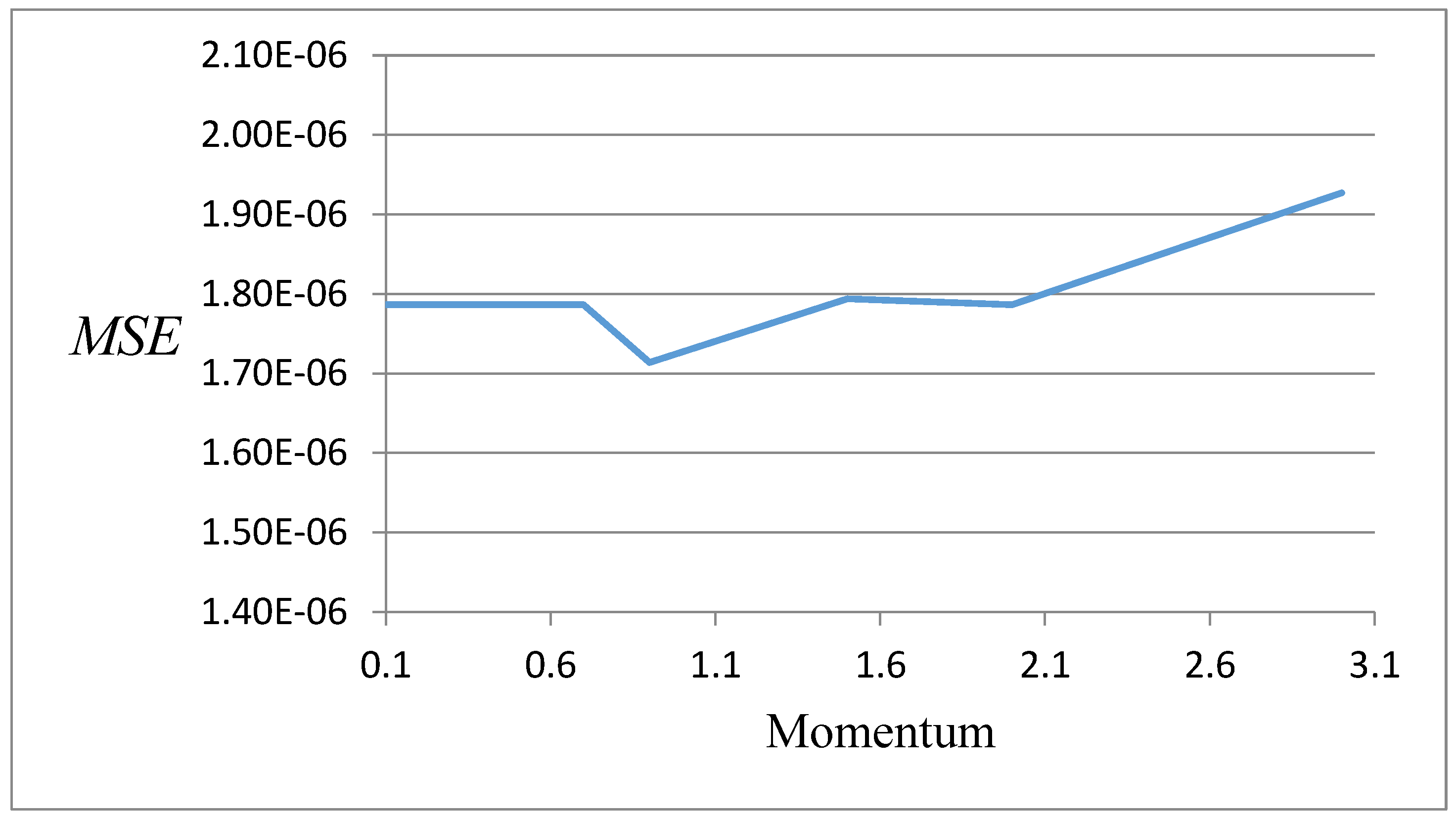
Appendix B. Results of the Selection of Network Learning Parameters
Appendix C
Appendix D
References
- Romanska-Zapala, A.; Bomberg, M.; Dechnik, M.; Fedorczak-Cisak, M.; Furtak, M. On Preheating of the Outdoor Ventilation Air. Energies 2020, 13, 15. [Google Scholar] [CrossRef] [Green Version]
- Romanska-Zapala, A.; Furtak, M.; Fedorczak-Cisak, M.; Dechnik, M. Cooperation of a Horizontal Ground Heat Exchanger with a Ventilation Unit During Winter: A Case Study on Improving Building Energy Efficiency. In Proceedings of the 3rd World Multidisciplinary Civil Engineering, Architecture, Urban Planning Symposium (Wmcaus 2018), Prague, Czech Republic, 18–22 June 2018; pp. 1757–8981. [Google Scholar]
- Romanska-Zapala, A.; Furtak, M.; Fedorczak-Cisak, M.; Dechnik, M. Need for Automatic Bypass Control to Improve the Energy Efficiency of a Building through the Cooperation of a Horizontal Ground Heat Exchanger with a Ventilation Unit during Transitional Seasons: A Case Study. In Proceedings of the 3rd World Multidisciplinary Civil Engineering, Architecture, Urban Planning Symposium (Wmcaus 2018), iop Conference Series-Materials Science and Engineering, Prague, Czech Republic, 18–22 June 2018; pp. 1757–8981. [Google Scholar]
- Romanska-Zapala, A.; Furtak, M.; Dechnik, M. Cooperation of Horizontal Ground Heat Exchanger with the Ventilation Unit during Summer—Case Study. In Proceedings of the World Multidisciplinary Civil Engineering-Architecture-Urban Planning Symposium—WMCAUS, Prague, Czech Republic, 12–16 June 2017. [Google Scholar]
- Fedorczak-Cisak, M.; Kotowicz, A.; Radziszewska-Zielina, E.; Sroka, B.; Tatara, T.; Barnaś, K. Multi-criteria Optimisation of the Urban Layout of an Experimental Complex of Single-family NZEBs. Energies 2020, 13, 1541. [Google Scholar] [CrossRef] [Green Version]
- Fedorczak-Cisak, M.; Kowalska-Koczwara, A.; Nering, K.; Pachla, F.; Radziszewska-Zielina, E.; Śladowski, G.; Tatara, T.; Ziarko, B. Evaluation of the Criteria for Selecting Proposed Variants of Utility Functions in the Adaptation of Historic Regional Architecture. Sustainability 2019, 11, 1094. [Google Scholar] [CrossRef] [Green Version]
- Romanska-Zapala, A.; Bomberg, M.; Yarbrough, D.W. Buildings with environmental quality management: Part 4: A path to the future NZEB. J. Build. Phys. 2019, 43, 3–21. [Google Scholar] [CrossRef]
- Yarbrough, D.W.; Bomberg, M.; Romanska-Zapala, A. Buildings with environmental quality management, part 3: From log houses to environmental quality management zero-energy buildings. J. Build. Phys. 2019, 42, 672–691. [Google Scholar] [CrossRef]
- Romanska-Zapala, A.; Bomberg, M.; Fedorczak-Cisak, M.; Furtak, M.; Yarbrough, D.; Dechnik, M. Buildings with environmental quality management, part 2: Integration of hydronic heating/cooling with thermal mass. J. Build. Phys. 2018, 41, 397–417. [Google Scholar] [CrossRef]
- Yarbrough, D.W.; Bomberg, M.; Romanska-Zapala, A. On the next generation of low energy buildings. Adv. Build. Energy Res. 2019, 1–8. [Google Scholar] [CrossRef]
- Bomberg, M.; Romanska-Zapala, A.; Yarbrough, D. Journey of American Building Physics: Steps Leading to the Current Scientific Revolution. Energies 2020, 13, 1027. [Google Scholar] [CrossRef] [Green Version]
- Radziszewska-zielina, E.; Śladowski, G. Proposal of the Use of a Fuzzy Stochastic Network for the Preliminary Evaluation of the Feasibility of the Process of the Adaptation of a Historical Building to a Particular Form of Use. IOP Conf. Ser. Mater. Sci. Eng. 2017, 245, 072029. [Google Scholar] [CrossRef]
- Romanska-Zapala, A.; Bomberg, M. Can artificial neuron networks be used for control of HVAC in environmental quality management systems? In Proceedings of the Central European Symposium of Building Physics, Prague, Czech Republic, 23–26 September 2019. [Google Scholar]
- Dudzik, M.; Romanska-Zapala, A.; Bomberg, M. A neural network for monitoring and characterization of buildings with Environmental Quality Management, Part 1: Verification under steady state conditions. Energies 2020, 13, 3469. [Google Scholar] [CrossRef]
- Bomberg, M.; Romanska-Zapala, A.; Yarbrough, D. Towards Integrated Energy and Indoor Environment Control in Retrofitted Buildings. Energies 2020, 2020070044, Preprints. [Google Scholar]
- Klepeis, N.E.; Nelson, W.C.; Ott, W.R.; Robinson, J.P.; Tsang, A.M.; Switzer, P.; Behar, J.V.; Hern, S.C.; Engelmann, W.H. The national human activity pattern survey (NHAPS): A resourcefor assessing exposure to environmental pollutants. J. Exposure Sci. Environ. Epidemiol. 2001, 11, 231–252. [Google Scholar] [CrossRef] [PubMed] [Green Version]
- Frontczak, M.; Wargocki, P. Literature survey on how different factorsinfluence human comfort in indoor environments. Build. Environ. 2011, 46, 922–937. [Google Scholar] [CrossRef]
- Heim, D.; Janicki, M.; Szczepanska, E. Thermal and visual comfort in a office building with double skin façade. In Proceedings of the 10th International Conference on Healthy Buildings 2012, Brisbane, Australia, 8–12 July 2012; Volume 2, pp. 1801–1806, ISBN 978-162748075-8. [Google Scholar]
- Szczepanska-Rosiak, E.; Heim, D.; Gorko, M. Visual comfort under real and theoretical, overcast and clear sky conditions. In Proceedings of the 13th Conference of the International Building Performance Simulation Association, BS 2013, Chambery, France, 26–28 August 2013; pp. 2765–2773. [Google Scholar]
- Wyon, D.P.; Andersen, I.; Lundqvist, G.R. The effects of moderateheat stress on mental performance. Scand. J. Work Environ. Health 1979, 5, 352–361. [Google Scholar] [CrossRef] [PubMed] [Green Version]
- World Energy Council. World Energy Resources 2013 Survey. 2013. Available online: http://www.worldenergy.org (accessed on 5 August 2018).
- Ma, G.; Liu, Y.; Shang, S. A Building Information Model (BIM) and Artificial Neural Network (ANN) Based System for Personal Thermal Comfort Evaluation and Energy Efficient Design of Interior Space. Sustainability 2019, 11, 4972. [Google Scholar] [CrossRef] [Green Version]
- Langevin, J.; Gurian, P.; Wen, J. Tracking the human-building interaction: A longitudinal field study of occupant behavior in air-conditioned offices. J. Environ. Psychol. 2015, 42, 94–115. Available online: http://www.sciencedirect.com/science/article/pii/S0272494415000225 (accessed on 15 April 2020). [CrossRef]
- ISO 7730:2005. Ergonomics of the Thermal Environment Analytical Determination and Interpretation of Thermal, Comfort Using Calculation of the PMV and PPD Indices and Local Thermal Comfort Criteria; International Standard Organization: Geneva, Switzerland, 2005; Available online: https://www.researchgate.net/publication/306013139_Ergonomics_of_the_thermal_environment_Determination_of_metabolic_rate (accessed on 10 May 2019).
- ISO 17772-1:2017. Energy Performance of Buildings—Indoor Environmental Quality—Part 1: Indoor Environmental Input Parameters for the Design and Assessment of Energy Performance of Buildings; ISO: Geneva, Switzerland, 2017.
- Mohamed Sahari, K.S.; Abdul Jalal, M.F.; Homod, R.Z.; Eng, Y.K. Dynamic indoor thermal comfort model identification based on neural computing PMV index. 4th International Conferenceon Energyand Environment 2013 (ICEE2013). IOP Publishing. IOP Conf. Ser. Earth Environ. Sci. 2013. [Google Scholar] [CrossRef]
- Sudoł-Szopińska, I.; Chojnacka, A. Determining Thermal Comfort Conditions in Rooms with the PMV and PPD Indices (EN); Określanie Warunków Komfortu Termicznego w Pomieszczeniach za Pomocą Wskaźników PMV i PPD (PL); Bezpieczeństwo Pracy: Nauka i praktyka; Centralny Instytut Ochrony Pracy—Państwowy Instytut Badawczy: Warsaw, Poland, 2007; Volume 5, pp. 19–23. [Google Scholar]
- Radziszewska-Zielina, E.; Czerski, P.; Grześkowiak, W.; Kwaśniewska-Sip, P. Comfort of Use Assessment in Buildings with Interior Wall Insulation based on Silicate and Lime System in the Context of the Elimination of Mould Growth. Arch. Civil Eng. 2020, 66, 2. [Google Scholar]
- U.S. Department of Energy. Buildings Energy Data Book. 2012. Available online: http://buildingsdatabook.eren.doe.gov/DataBooks.aspx (accessed on 15 August 2018).
- Ferreira, P.M.; Sergio, M.S.; Ruano, A.; Negrier, A.; Eusébio, C. Neural Network PMV Estimation for Model-Based Predictive Control of HVAC Systems. In Proceedings of the WCCI 2012 IEEE World Congress on Computational Intelligence, Brisbane, Australia, 10–15 June 2012. [Google Scholar] [CrossRef] [Green Version]
- Jin, W.; Feng, Y.; Zhou, N.; Zhong, X. A Household Electricity Consumption Algorithm with Upper Limit. In Proceedings of the 2014 International Conference on Wireless Communication and Sensor Network, Wuhan, China, 13–14 December 2014; WCSN 2014 Organizing Committee: Beijing, China, 2014; pp. 431–434. [Google Scholar]
- Dexter, A. Intelligent buildings: Fact or fiction? HVAC&R Res. 1996, 2, 105–106. [Google Scholar]
- Radziszewska-Zielina, E.; Rumin, R. Analysis of investment profitability in renewable energy sources as exemplified by a semi-detached house. In Proceedings of the International Conference on the Sustainable Energy and Environment Development, Kraków, Poland, 17–19 May 2016; SEED; AGH; Center of Energy: Kraków, Poland. [Google Scholar]
- Ding, Y.; Tian, Q.; Fu, Z.; Li, M.; Zhu, N. Influence of indoor design air parameters on energy consumption of heating and air conditioning. Energy Build. 2013, 56, 78–84. [Google Scholar] [CrossRef]
- Romanska-Zapala, A.; Kowalska-Koczwara, A.; Korchut, A.; Stypula, K.; Melcer, J.; Kotrasova, K. Psychomotor conditions of bus drivers subjected to noise and vibration in the working environment. In Proceedings of the MATEC Web of Conferences, Conference on Dynamics of Civil Engineering and Transport Structures and Wind Engineering (DYN-WIND), Trstena, Slovakia, 21–25 May 2017. [Google Scholar] [CrossRef] [Green Version]
- Korchut, A.; Korchut, W.; Kowalska-Koczwara, A.; Romanska-Zapala, A.; Stypula, K.; Vestroni, F.B.E.; Romeo, F.; Gattulli, V. The relationship between psychomotor efficiency and selected personality traits of people exposed to noise and vibration stimuli. Procedia Eng. 2017, 199, 200–205. [Google Scholar] [CrossRef]
- Korchut, A.; Kowalska-Koczwara, A.; Romanska-Zapala, A.; Stypula, K. Relationship Between Psychomotor Efficiency and Sensation Seeking of People Exposed to Noise and Low Frequency Vibration Stimuli. In Proceedings of the IOP Conference Series-Materials Science and Engineering, World Multidisciplinary Civil Engineering-Architecture-Urban Planning Symposium (WMCAUS), Prague, Czech Republic, 12–16 June 2017. [Google Scholar]
- Liu, W.; Lian, Z.; Zhao, B. A neural network evaluation model for individual thermal comfort. Energy Build. 2007, 39, 1115–1122. [Google Scholar] [CrossRef]
- Kim, J.; Zhou, Y.; Schiavon, S.; Raftery, P.; Brager, G. Personal comfort models: Predicting individuals’ thermal preference using occupant heating and cooling behavior and machine learning. Build. Environ. 2018, 129, 96–106. [Google Scholar] [CrossRef] [Green Version]
- Von Grabe, J. Potential of artificial neural networks to predict thermal sensation votes. Appl. Energy 2016, 161, 412–424. [Google Scholar] [CrossRef]
- Buratti, C.; Vergoni, M.; Palladino, D. Thermal comfort evaluation within non-residential environments: Development of Artificial Neural Network by using the adaptive approach data. 6th International Building Physics Conference, IBPC 2015. Energy Procedia 2015, 78, 2875–2880. [Google Scholar] [CrossRef] [Green Version]
- Zocca, V.; Spacagna, G.; Slater, D.; Roelants, P. Python Deep Learning; Packt Publishing: Birmingham, UK, 2017; ISBN1 1786464454. ISBN2 978-1786464453. [Google Scholar]
- Fanger, P. Thermal Comfort. Analysis and Applications in Environmental Engineering; Danish Technical Press: Copenhagen, Denmark, 1970; Available online: https://www.researchgate.net/publication/35388098_Thermal_Comfort_Analysis_and_Applications_in_Environment_Engeering (accessed on 20 October 2018).
- ANSI; ASHRAE. ANSI/ASHRAE 55–2013: Thermal Environmental Conditions for Human Occupancy; American Society of Heating; Refrigerating and Air Conditioning Engineers: Atlanta, GA, USA, 2013. [Google Scholar]
- Sharma, A.; Tiwari, R. Evaluation of data for developing an adaptive model of thermal comfort and preference. Environmentalist 2007, 27, 73–81. [Google Scholar] [CrossRef]
- Nicol, J.; Humphreys, M. Adaptive thermal comfort and sustainable thermal standards for buildings. Energy Build. 2002, 34, 563–572. [Google Scholar] [CrossRef]
- Auenberg, F.; Stein, S.; Rogers, A. A personalised thermal comfort model using a Bayesian Network. IJCAI 2015, 2015, 2547–2553. [Google Scholar]
- Van Hoof, J. Forty years of Fanger’s model of thermal comfort: Comfort for all? Indoor Air 2008, 18, 182–201. [Google Scholar] [CrossRef]
- Alfano, F.; Palella, B.; Riccio, G. The role of measurement accuracy on the thermal environment assessment by means of PMV index. Build. Environ. 2011, 46, 1361–1369. [Google Scholar] [CrossRef]
- Neto, A.; Fiorelli, F.A.S. Comparison between detailed model simulation and artificial neural network for forecasting building energy consumption. Energy Build. 2008, 40, 2169–2176. [Google Scholar] [CrossRef]
- Kalogirou, S.; Bojic, M. Artificial neural networks for the prediction of the energy consumption of a passive. Energy 2000, 25, 479–491. [Google Scholar] [CrossRef]
- Javeed Nizami, S.; Al-Garni, A. Forecasting electric energy consumption using neural networks. Energy Policy 1995, 23, 1097–1104. [Google Scholar] [CrossRef]
- Yokoyama, R.; Wakui, T.; Satake, R. Prediction of energy demands using neural network with model identification by global optimization. Energy Convers. Manag. 2009, 50, 319–327. [Google Scholar] [CrossRef]
- Buratti, C.; Barbanera, M.; Palladino, D. An original tool for checking energy performance and certification of buildings by means of Artificial Neural Networks. Appl. Energy 2014, 120, 125–132. [Google Scholar] [CrossRef]
- Buratti, C.; Lascaro, E.; Palladino, D.; Vergoni, M. Building behavior simulation by means of Artificial Neural Network in summer conditions. Sustainability 2014, 6, 5339–5353. [Google Scholar] [CrossRef] [Green Version]
- Chen, Y.; Liu, J.; Li, X.; Yin, B.; Wu, X. HVAC System Energy Consumption Prediction of Green Office Building Based on ANN Method. Build. Energy Sav. 2017, 10, 1–5. [Google Scholar]
- Dutta, N.N.; Das, T. Artificial intelligence techniques for energy efficient H.V.A.C. system design. In Proceedings of the International Conference on Emerging Technologies for Sustainable and Intelligent HVAC&R Systems, Kolkata, India, 27–28 July 2018. [Google Scholar]
- Marvuglia, A.; Messineo, A.; Nicolosi, G. Coupling a neural network temperature predictor and a fuzzy logic controller to perform thermal comfort regulation in an office building. Build. Environ. 2014, 72, 287–299. [Google Scholar] [CrossRef]
- Palladino, D.; Lascaro, E.; Orestano, F.C.; Barbanera, M. Artificial Neural Networks for the Thermal Comfort Prediction in University Classrooms: An Innovative Application of Pattern Recognition and Classification Neural Network. In Proceedings of the 17th CIRIAF National Congress Sustainable Development, Human Health and Environmental Protection, Perugia, Italy, 6–7 April 2017. [Google Scholar]
- Zhao, Y.; Genovese, P.; Li, Z. Intelligent Thermal Comfort Controlling System for Buildings Based on IoT and AI. Future Internet 2020, 12, 30. [Google Scholar] [CrossRef] [Green Version]
- Ghahramani, A.; Galicia, P.; Lehrer, D.; Varghese, Z.; Wang, Z.; Pandit, Y. Artificial Intelligence for Efficient Thermal Comfort Systems: Requirements, Current Applications and Future Directions. Front. Built Environ. 2020. [Google Scholar] [CrossRef]
- I.O. for Standardization (ISO). ISO 7730: Moderate Thermal Environments—Determination of the PMV and PPD Indices and Specification of the Conditions for Thermal Comfort; International Organization for Standardization: Geneva, Switzerland, 1994. [Google Scholar]
- Kang, J.; Kim, Y.; Kim, H.; Jeong, J.; Park, S. Comfort sensing system for indoor environment. In Proceedings of the International Conference on Solid State Sensors and Actuators, Chicago, IL, USA, 19 June 1997; pp. 311–314. [Google Scholar]
- Bedford, T.; Warner, C. The globe thermometer in studies of heating and ventilation. J. Hyg. (Lond.) 1934, 34, 458–473. [Google Scholar] [CrossRef] [PubMed] [Green Version]
- Cena, K.; Clark, J. Bioengineering, Thermal Physiology and Comfort, Ser. Studies in Environmental Science; Elsevier: Amsterdam, The Netherlands, 1981; Volume 10. [Google Scholar]
- Demuth, H.; Beale, M.; Hagan, M. Neural Network Toolbox 6 User’s Guide; The MathWorks Inc.: Natick, MA, USA, 2009. [Google Scholar]
- Mathworks Documentation: Mapminmax. Available online: https://www.mathworks.com/help/deeplearning/ref/mapminmax.html (accessed on 21 February 2019).
- Matlab and Automatic Target Normalization: Mapminmax. Don’t Trust Your Matlab Framework! Available online: https://neuralsniffer.wordpress.com/2010/10/17/matlab-and-automatic-target-normalization-mapminmax-dont-trust-your-matlab-framework/ (accessed on 21 February 2019).
- Dudzik, M.; Mielnik, R.; Wrobel, Z. Preliminary analysis of the effectiveness of the use of artificial neural networks for modelling time-voltage and time-current signals of the combination wave generator. In Proceedings of the 2018 International Symposium on Power Electronics, Electrical Drives, Automation and Motion (Speedam), Amalfi, Italy, 20–22 June 2018. [Google Scholar]
- Dudzik, M.; Stręk, A.M. ANN Architecture Specifications for Modelling of Open-Cell Aluminum under Compression. Math. Probl. Eng. 2020, 2020. [Google Scholar] [CrossRef] [Green Version]
- Szymenderski, J.; Typańska, D. Control model of energy flow in agricultural biogas plant using SCADA software. In Proceedings of the 17th International Conference Computational Problems of Electrical Engineering (CPEE), Sandomierz, Poland, 9–11 October 2016; pp. 1–4. [Google Scholar] [CrossRef]
- Budnik, K.; Szymenderski, J.; Walowski, G. Control and Supervision System for Micro Biogas Plant. In Proceedings of the 19th International Conference Computational Problems of Electrical Engineering, Banska Stiavnica, Slovakia, 9–12 September 2018; pp. 1–4. [Google Scholar] [CrossRef]
- Hagan, M.; Demuth, H.; Beale, M.; De Jesus, O. Neural Network Design, 2nd ed. 2014; eBook.
- Dudzik, M. Contemporary Methods of Designing, Validation and Modeling of the Phenomena of Electrical Traction (En), Współczesne Metody Projektowania, Weryfikacji Poprawności I Modelowania Zjawisk Trakcji Elektrycznej (PL): Monochart, Politechnika Krakowska im. Tadeusza Kościuszki. Kraków, Wydaw. PK, 2018. 187 s., Monografie Politechniki Krakowskiej. Inżynieria Elektryczna i Komputerowa; Politechnika Krakowska: Krakow, Poland, 2018; ISBN 978-83-65991-28-7. [Google Scholar]
- Tomczyk, K. Special signals in the Calibration of Systems for Measuring Dynamic Quantities. Measurement 2014, 49, 148–152. [Google Scholar] [CrossRef]
- Layer, E.; Tomczyk, K. Determination of Non-Standard Input Signal Maximizing the Absolute Error. Metrol. Meas. Syst. 2009, XVII, 199–208. [Google Scholar]
- Tomczyk, K. Levenberg-Marquardt Algorithm for Optimization of Mathematical Models according to Minimax Objective Function of Measurement Systems. Metrol. Meas. Syst. 2009, XVI, 599–606. [Google Scholar]
- Tomczyk, K.; Piekarczyk, M.; Sokal, G. Radial Basis Functions Intended to Determine the Upper Bound of Absolute Dynamic Error at the Output of Voltage-Mode Accelerometers. Sensors 2019, 19, 1–15. [Google Scholar] [CrossRef] [Green Version]
- Tomczyk, K. Impact of uncertainties in accelerometer modelling on the maximum values of absolute dynamic error. Measurement 2016, 80, 71–78. [Google Scholar] [CrossRef]
- Latka, D.; Matysek, P. Determination of Mortar Strength in Historical Brick Masonry Using the Penetrometer Test and Double Punch Test. Materials 2020, 13, 2873. [Google Scholar] [CrossRef]
- Latka, D.; Matysek, P. The estimation of compressive stress level in brick masonry using the flat-jack method. International Conferenceon analytical models and new concepts in concrete and masonry structures. Procedia Eng. 2017, 193, 266–272. [Google Scholar] [CrossRef]
- jared.langevin@lbl.gov, Langevin Data Legend. One Year Occupant Behavior/Environment Data for Medium U.S. Office. Available online: https://openei.org/datasets/dataset/one-year-behavior-environment-data-for-medium-office (accessed on 16 April 2020).
- Madsen, K.; Nielsen, H.; Tingleff, O. Methods for Non-Linear Least Squares Problems, 2nd ed.; Informatics and Mathematical Modelling Technical University of Denmark: Lyngby, Denmark, 2004; Available online: http://www2.imm.dtu.dk/pubdb/views/edoc\_download.php/3215/pdf/imm3215.pdf (accessed on 15 October 2018).
- Philip, S. Pearson’s correlation coefficient. BMJ 2012, 345, e4483. [Google Scholar] [CrossRef] [Green Version]
- Dudzik, M.; Drapik, S.; Jagiello, A.; Prusak, J. The selected real tramway substation overload analysis using the optimal structure of an artificial neural network. In Proceedings of the 2018 International Symposium on Power Electronics, Electrical Drives, Automation and Motion (SPEEDAM), Amalfi, Italy, 20–22 June 2018. [Google Scholar]
- Radziszewska-Zielina, E.; Kania, E.; Śladowski, G. Problems of the Selection of Construction Technology for Structures of Urban Aglomerations. Arch. Civil Eng. 2018, 64, 55–71. [Google Scholar] [CrossRef]
- Nanthakumar, C.; Vijayalakshmi, S. Construction of inter quartile range (IRQ) control chart using process capability for mean using range. Int. J. Mod. Sci. Eng. Technol. 2015, 2, 8. [Google Scholar]
- Estep, D.; Larson, M.G.; Williams, R. Estimating the Error of Numerical Solutions of Systems of Reaction–Diffusion Equations; Memoirs of the American Mathematical Society; American Mathematical Society: Providence, RI, USA, 2000. [Google Scholar] [CrossRef]
- Albatayneh, A.; Alterman, D.; Page, A.; Moghtaderi, B. The Impact of the Thermal Comfort Models on the Prediction of Building Energy Consumption. Sustainability 2018, 10, 3609. [Google Scholar] [CrossRef] [Green Version]
- Ruano, A.E.; Ferreira, P.M. Neural Network based HVAC Predictive Control. In Proceedings of the Preprints of the 19th World Congress the International Federation of Automatic Control, Cape Town, South Africa, 24–29 August 2014; pp. 3617–3622. [Google Scholar]
- Sowa, S. Lighting control systems using daylight to optimise energy efficiency of the building. In Proceedings of the 2019 Progress in applied electrical engineering (PAEE), Koscielisko, Poland, 17–21 June 2019. [Google Scholar]


| Input Argument | Category | Name | Type | Units (if Applicable) | Range of the Variable |
|---|---|---|---|---|---|
| Environment | Indoor ambient temp. | Continuous | °C | [16.76, 25.79] | |
| Environment | Indoor relative humidity | Continuous | % | [14.25, 72.57] | |
| Environment | Indoor air velocity | Continuous | m/s | [0.026, 0.031] | |
| Environment | Indoor mean radiant temp. | Continuous | °C | [16.76, 25.79] | |
| Environment | Indoor CO2 | Continuous | ppm | [1.2, 876.7] | |
| Environment | Outdoor ambient temp. | Continuous | °C | [–11, 35] | |
| Environment | Outdoor relative humidity | Continuous | % | [21, 100] | |
| Environment | Outdoor air velocity | Continuous | m/s | [0, 12.5] | |
| Personal characteristics | Clothing level | Continuous | CLO | [0.22, 0.99] | |
| Personal characteristics | Clothing level (+ chair) | Continuous | CLO | [0.32, 1.09] | |
| Personal characteristics | Gender | Discrete | -- | 2 | |
| Personal characteristics | Age | Discrete | Years | 32 | |
| Personal characteristics | Office type | Discrete | -- | 3 | |
| Personal characteristics | Floor number | Discrete | -- | 1 | |
| Behavior | Current thermostat cooling setpoint | Continuous | °C | [15.95, 24.13] | |
| Behavior | Base thermostat cooling setpoint | Continuous | °C | [23.88, 25.55] | |
| Behavior | Current thermostat heating setpoint | Continuous | °C | [22.50, 26.66] | |
| Behavior | Base thermostat heating setpoint | Continuous | °C | [15.55, 24.44] | |
| General | Occupancy 1 | Discrete | -- | [0, 1] | |
| General | Occupancy 2 | Discrete | -- | [0, 1] |
| Output Value | Category | Name | Type | Units (If Applicable) |
|---|---|---|---|---|
| MODEL | Predicted Mean Vote (PMV) | Continuous | Limited to [−3,3] |
| Learning Parameter | Value |
|---|---|
| performance function goal | 0 |
| minimum performance gradient | 10−10 |
| maximum validation failures | 12 |
| maximum number of epochs to train | 100,000 |
| learning rate | 0.01 |
| momentum | 0.9 |
| 5 | |
| 0.106 | |
| 0.029 | |
| 0.025 | |
| 0.043 | |
| 0.018 | |
| 0.070 | |
| 0.047 | |
| 0.024 | |
| 0.031 | |
| 0.072 |
| Value | |
| Training stage | 0.99998 |
| Validation stage | 0.99999 |
| Testing stage | 0.99999 |
| All data | 0.99998 |
© 2020 by the author. Licensee MDPI, Basel, Switzerland. This article is an open access article distributed under the terms and conditions of the Creative Commons Attribution (CC BY) license (http://creativecommons.org/licenses/by/4.0/).
Share and Cite
Dudzik, M. Towards Characterization of Indoor Environment in Smart Buildings: Modelling PMV Index Using Neural Network with One Hidden Layer. Sustainability 2020, 12, 6749. https://doi.org/10.3390/su12176749
Dudzik M. Towards Characterization of Indoor Environment in Smart Buildings: Modelling PMV Index Using Neural Network with One Hidden Layer. Sustainability. 2020; 12(17):6749. https://doi.org/10.3390/su12176749
Chicago/Turabian StyleDudzik, Marek. 2020. "Towards Characterization of Indoor Environment in Smart Buildings: Modelling PMV Index Using Neural Network with One Hidden Layer" Sustainability 12, no. 17: 6749. https://doi.org/10.3390/su12176749
APA StyleDudzik, M. (2020). Towards Characterization of Indoor Environment in Smart Buildings: Modelling PMV Index Using Neural Network with One Hidden Layer. Sustainability, 12(17), 6749. https://doi.org/10.3390/su12176749