Article

Global Emission Taxes and Port Privatization Policies under International Competition

1
Department of Economics and Trade, Dalian Maritime University, 1 Linghai Road, Dalian 116026, China
2
Department of Economics, Chonnam National University, 77 Yongbong-Ro, Bukgu, Gwangju 61186, Korea
*
Author to whom correspondence should be addressed.
Sustainability 2020, 12(16), 6595; https://doi.org/10.3390/su12166595
Submission received: 6 July 2020 / Revised: 6 August 2020 / Accepted: 13 August 2020 / Published: 14 August 2020

Abstract

:
This study considers two asymmetric ports under international competition in which each country has a hub port and a private manufacturer and investigates strategic interactions between port privatization and emission tax policies. We emphasize the key role of the relative market size between the two countries and show that in a privatization choice game, port privatization is a dominant strategy in a larger country, but it will be chosen by a smaller country only if its relative market size is not so small. We also show that the coordination of global emission taxes before privatization choices can induce the equilibrium of the game to be globally optimal when the emission tax is relatively high. This finding provides an important policy implication on the climate change that coordinated global environmental policy is imperatively required in the port privatization policy.
JEL Classifications:
D43; F18; H23; L33

1. Introduction

Since the 1970s, as many countries have moved toward the privatization of public ports, the private operation of port facilities has become increasingly common worldwide. According to the general category (ownership structure) defined by The World Bank (2007), service/tool (public) ports and landlord ports are generally considered to have a strong focus on public objectives (i.e., maximizing consumer surplus), while fully private ports will mainly focus on profits only [1]. In accordance with the global trend of liberalization and deregulation, the privatization of public ports is regarded as a policy option that can raise port competitiveness [2,3,4]. In recent years, many researchers have expressed concern about the impact of the port privatization on the environment since the ownership structure of ports has been recognized as one of the most important determinants of port usage fees and emissions that influence port efficiency and environmental protection.
Owing to the explosive development of international shipping, the emissions of ports account for a significant share of global emissions of greenhouse gases. According to data from the Hong Kong Environmental Protection Department in 2017, international shipments are the largest source of respirable suspended particulate (RSP), NOx and SO2, representing about 34%, 37% and 52% of the RSP, NOx and SO2 in Hong Kong for that year [5]. Hence, governments should globally adjust their privatization and environmental policies under international open competition.
To achieve the goal of carbon emission reduction, many countries have implemented carbon tax policies, such as the Netherlands, Sweden, Finland and Norway in Europe. According to data from the International Maritime Organization (IMO), the annual carbon dioxide emissions of the international shipping industry account for about 3% of the total global emissions in 2014. It is estimated that if no further supervision is introduced, this number will jump to 18% in 2050 [6]. Thus, the EU Commission has been committed to imposing a maritime carbon tax since 2012. The EU has monitored the carbon emissions of ships over 5000 tons since 2018, which can be seen as the first step towards a maritime carbon tax.
On the one hand, earlier studies of the privatization policy examined the ownership structure of a public port in a competitive market and the effect of the port privatization on performances. At the political level, many governments consider the privatization or corporatization of public ports as a political option to increase the competitive position of their ports [2,7,8]. For instance, governance, meaning port ownership and management, is one of the factors that influence the performance and efficiency of ports [9]. Port privatization not only improves efficiency and performance, but also increases trade volume [10,11,12,13,14,15]. Moreover, the link between port efficiency and export variety for a broad cross-section of countries, and the effect of airport privatization on per-connecting-passenger charges are also analyzed [16,17,18]. Thus, the door privatization has positive effects on cost-effectiveness and technical efficiency [19,20,21,22].
Further, several theoretical works examined the port privatization and found some interesting results in an international competition. For example, both privatization of the two airports is an equilibrium in an international competition. However, no privatization leads to greater welfare, even though a smaller country has a larger incentive to adopt a privatization policy [4,23,24]. Moreover, using a game theory approach, the effects of port ownership structure on port tariffs, investments, profits, and well-being in an international market are investigated [25,26]. They showed that a smaller country’s government is more likely to privatize its ports, whereas the larger country’s government is more likely to nationalize its ports to protect its domestic market [26]. Finally, the port ownership strategy alters according to the exporting firm’s competition under free trade or trade tariff regime [27,28]. However, these researchers did not take the environmental concerns of the port privatization policy into account.
On the other hand, recent studies of a mixed oligopoly market have explored the relationship between privatization policy and environmental regulation in both domestic and international markets. Since the pioneering studies examined the effects of privatization policy on the environment in a mixed market, the past decade has witnessed an increasing volume of research on the environment in a mixed oligopoly framework [29,30]. In the context of a domestic market, Beladi and Chao showed that full privatization harms the environment in a monopoly market [30]. Naito and Ogawa found that the optimal level of environmental regulation critically depends on the degree of privatization and their relationship is not monotonous [31]. Xu et al. compared a Cournot with a Bertrand duopoly in a differentiated mixed market wherein both emission taxes and privatization policies are strategically substitutable [32]. Ye and Zhao also examined the impact of public firms in mixed oligopolies on environmental protection and regulation [33]. In particular, Tseng and Pilcher firstly proposed a ship emission tax in port/berth and considered it valuable and viable at a policy level and Zheng et al. investigated a possible port emission regulation impacted by incomplete information [34,35]. In the context of an international market, Abe et al. investigated the effect of bilateral trade liberalization and environmental regulation on national welfare and the environment [36]. Sheng et al. compared the economic and environmental effects of a unilateral maritime emission regulation with those of a uniform maritime emission regulation [37]. Xu and Lee also examined the strategic interaction between two governments under different privatization policies with import tariffs and environmental taxes [38]. Finally, Cui and Notteboom investigated the interaction between emission taxes and port privatization under different competition modes and showed that port privatization has a non-monotonous effect on a port’s environmental damage [39]. We show an overview of the literature in the following Table 1.
Although these findings on the relationship between privatization and emission tax policies provide interesting insights, the literature has scarcely examined the interaction between port privatization and emission taxes in an international mixed market. In particular, if two countries have asymmetric market sizes, it crucially brings about engaging in strategic interactions, as shown in Matsushima and Takauchi [26]. In this paper, we incorporate environmental perspective and explore the relationship between port privatization policy and environmental tax regulation under international competition. In particular, we extended Matsushima and Takauchi and Cui and Notteboom by considering port privatization choice games and different types of environmental taxes in this paper, in which the pollutants occur during port operations [26,39]. Further, we assume that two governments impose an emission tax on their domestic port because both ports charge usage fees to the exports of the firms during international transactions. On the contrary, if the emission taxes are imposed on shipping firms, however, it will be absorbed in usage fee, especially, under public port. This is different from Abe et al. which considered the effect of emission taxes which are imposed on shipping firms on national welfare and the environment [36]. Taking port emissions between two countries that have asymmetric market sizes into considerations, we examine strategic policy interactions between the two governments in this paper. We examine three different privatization policies: (i) no privatization case in which both governments keep their port public, (ii) bilateral privatization case in which both governments privatize their ports simultaneously and (iii) unilateral privatization case in which only one of the two governments privatizes its ports. Then, we compare port usage fees, emission taxes and welfare levels among those cases. Finally, we consider a port privatization choice game between the two countries and examine the role of global emission taxes in which both countries can coordinate emission taxes.
We show that the equilibrium outcomes under an international mixed market depend on the emission tax and privatization policies of each country and find the key role of the relative market size between the two countries in determining the port privatization and emission tax policies. These results are contrasting to Matsushima and Takauchi who show that per-unit trade cost is the key determinant of the organizational structure when the market size in the two countries is the same [26]. Our main findings are as follows: First, the optimal emission tax level is always higher than the marginal environmental damage in a larger country, while it may be lower (higher) than the marginal environmental damage when the relative market size is small (large) in a smaller country. This result is opposite to the previous findings. In particular, it is in contract to the finding in Cui and Notteboom who examined the unilateral market with port privatization and showed that the optimal emission tax can be always higher than the marginal environmental damage [39]. Hence, each country can use emission taxes to substitute its privatization policy. Further, the optimal tax rate is lower than marginal environmental damage when there is imperfect competition either under a private or mixed market in the literature of emission taxes [32,38,40].
Second, a unilaterally privatized port sets the highest port usage fee and obtains the greatest domestic welfare when the other country keeps its port public. Thus, there may be excessive initiatives in port privatization policies. This finding of excessive privatization is consistent with the previous findings in an international competition under competitive privatization [4,23,24,26,41]. Matsushima and Takauchi found that the smaller country’s government is more likely to privatize its ports, whereas the larger country’s government is more likely to nationalize its ports to protect its domestic market [26]. In particular, Matsushima and Takauchi showed that per-unit trade cost is the key determinant of the organizational structure. However, with the consideration of emission taxes, our analysis shows that port privatization policy is a dominant strategy for the larger country, while the smaller country chooses to nationalize (privatize) its ports when its relative market size is relatively (not so) small [26]. This is because the country with a privatized port can use emission taxes to substitute privatization policy strategically. In this situation, each country will take aggressive choices in the port privatization policy.
Third, no privatization yields the greatest global welfare, but either bilateral or unilateral privatization could be the equilibrium in an endogenous choice game of port privatization policies, depending on the relative market size. Thus, the equilibrium of the port privatization choice game under international competition may yield a suboptimal result from a global perspective. This result is consistent with Czerny et al. and Matsushima and Takauchi who found that no privatization may lead to greater welfare, but the equilibrium may not be socially desirable [4,26].
Finally, the equilibrium in a port privatization choice game may not be globally optimal even under the coordinated emission taxes after privatization choices. However, the global emission taxes before privatization choices can induce the equilibrium of the game to be globally optimal when the emission tax is relatively high. On one hand, if both countries can coordinate global emission taxes after port privatization choices, no privatization can be a unique equilibrium in a port privatization choice game, while bilateral port privatization yields the greatest global welfare in this case. That is, no privatization leads to the smallest global welfare if the coordinated global emission taxes are determined after the privatization policy, which is in contrast to the results without coordination of emission taxes. On the other hand, the global emission taxes before privatization choices can induce the equilibrium of the privatization choice game to be globally optimal when the global emission tax is relatively high. Therefore, it is globally desirable for both countries to coordinate a higher level of the global emission tax before the countries choose the option of privatization of public ports. This finding provides an important global policy implication on the climate change that coordinated environmental policy between the countries is imperatively required in the port privatization policies.
The remainder of this paper is organized as follows: Section 2 introduces the basic model. Section 3 analyzes four scenarios under international competition: one bilateral privatization case, two unilateral privatization cases and one no privatization case, respectively. Section 4 compares the results of usage fees, emission taxes and welfare and then considers a port privatization choice game between two countries. Section 5 examines the coordination of emission taxes before and after the decision of port privatization in an endogenous choice game, where both countries cooperate and maximize global welfare. Section 6 concludes the study.

2. The Model

Suppose that there are two countries in the world: one is a larger country (country i) and the other is a smaller country (country j). Each country has a (either public or private) port and a private manufacturer that supplies homogeneous products to both markets. The consumption of products in country i is denoted as Q i = q h i + q e j , where q h i denotes the quantity supplied by the firm in country i and q e j denotes the exports from the firm in country j to market i.
The inverse demand function in each market is p i = 1 Q i and p j = 1 1 b Q j , respectively, where p i is the market price in country i and b denotes the relative market size of country j compared with country i ( j ) . We assume that 0 < b 1 ; that is, the market size of j is smaller than or equal to that of i and the relative market size of country j is small (large) when b is small (large). Given the quantities supplied by the two firms, the consumer surplus in each market is given as C S i = 1 2 Q i 2 and C S j = 1 2 b Q j 2 , respectively.
When a firm exports, it must use the two ports in each country with payments, which incurs a per-unit shipping fee (transport cost) from competitive shippers. For simplification, no firm incurs any costs other than those associated with transportation. Thus, the production cost is assumed to be zero, while the export cost of firm i in country i is τ + f i + f j , where τ is the per-unit shipping fee (exogenously given by competitive shippers) and f i is the per-unit fee for the usage of the port in country i. For the positive equilibrium outcomes in the analysis, we assume that τ [ 0 , 1 4 ) . The profit of the private manufacturer in each county is the sum of the profits in the two markets:
π i = p i q h i + ( p j τ f i f j ) q e i , π j = p j q h j + ( p i τ f i f j ) q e j .
We assume that pollutants occur during port operations in this study, which are proportional to the total traffic in each port, that is, q e i + q e j . In particular, we assume that the traffic emits the same pollutants and damage, which is quadratic in total traffics, E D i = E D j = ( q e i + q e j ) 2 2 . Note that we use the quadratic environment damage function to make sure that the second-order condition is satisfied in this study, which is also commonly used in the mixed market literature [29,30,32,36,42,43]. Each government imposes emission taxes on the port to the traffic and the tax revenue of the government in county i is T i = t i ( q e i + q e j ) , where t i > 0 and i j . The owner of the port in each country does not incur any operating cost, but must pay the emission tax. In addition, port revenue in country i comes from exports from country i to country j and imports from country j to country i. Then, the profit of the port in each country is given as:
R i = ( f i t i ) ( q e i + q e j ) , R j = ( f j t j ) ( q e i + q e j ) .
Domestic welfare is the sum of the consumer surplus, domestic industry profits, port profits and tax revenue minus environmental damage:
W i = C S i + π i + R i + T i E D i , W j = C S j + π j + R j + T j E D j .
Finally, we define global welfare as the sum of these domestic welfare levels in Equation (3), that is, W ¯ = W i + W j .
We consider two types of port ownership in each country: public or private port. A port is assumed to maximize domestic welfare in Equation (3) under public ownership, while it maximizes port profits in Equation (2) under private ownership. We then examine the welfare effect of the privatization choice of the two countries in the four policy regimes: (i) both ports are nationalized (NN case), (ii) the port in the smaller country j is privatized (NP case), (iii) the port in the larger country i is privatized (PN case) and (iv) both ports are privatized (PP case).
The timing of this game is as follows: In the first stage, each government chooses whether to privatize its port simultaneously. In the second stage, each government chooses its emission tax to maximize its domestic welfare. In the third stage, each port chooses its usage fees to maximize its objectives. In the fourth stage, each manufacturer competes in quantities in a Cournot fashion. The subgame perfect Nash equilibrium is solved by backward induction.

3. The Analysis

In the final stage, each private firm simultaneously sets its quantities to produce and export in the two markets under international competition. From the first-order conditions of the private firm, which maximizes Equation (1), we have the following equilibrium outputs:
q h i = 1 + τ + f i + f j 3 ,   q e i = b ( 1 2 τ 2 f i 2 f j ) 3 ,   q h j = b ( 1 + τ + f i + f j ) 3 ,   q e j = 1 2 τ 2 f i 2 f j 3 .
A few remarks are in order. First, the shipping fee increases the domestic firm’s production in each country, but decreases its exports to the other country, that is, q h k τ > 0 and q e k τ < 0 , where k = i , j . Second, port usage fees also increase the domestic firm’s production in each country, but decrease its exports to the other country, that is, q h i f k > 0 , q h j f k > 0 , q e i f k < 0   and   q e j f k < 0 , where k = i , j . Third, the market size of country j is independent of the consumption of products in the other country i, while it increases the consumption of products in its own country j, that is, q h i b = 0 , q e j b = 0 , q h j b > 0   and   q e i b > 0 . Finally, the emission tax is independent of the firm’s production and exports because the tax effect is already embedded in the port usage fee schedule under different ownership types, that is, q h i t k = 0 , q h j t k = 0 , q e i t k = 0   and   q e i t k = 0 , where k = i , j .
Then, we have the profits of the port and domestic welfare in each country as follows:
R i = ( 1 + b ) ( 1 2 τ 2 f i 2 f j ) ( f i t i ) 3 , R j = ( 1 + b ) ( 1 2 τ 2 f i 2 f j ) ( f j t j ) 3 , W i = A 1 + 2 f i ( 5 7 τ + 3 b 6 b τ + 2 b 2 4 b 2 τ ) ( 13 + 12 b + 4 b 2 ) f i 2 + 2 f j ( 2 + 2 b 2 τ 4 b 2 τ ) ( 1 + 4 b 2 ) f j 2 2 f i f j ( 7 + 6 b + 4 b 2 ) 18 , W j = A 2 2 f i ( 2 4 b 2 b 2 4 τ + 5 b τ + 4 b 2 τ ) + ( 4 5 b 4 b 2 ) f i 2 + 2 f j ( 1 + 7 b + 2 b 2 2 τ 11 b τ 4 b 2 τ ) ( 8 + 17 b + 4 b 2 ) f j 2 2 f i f j ( 2 + 11 b + 4 b 2 ) 18 ,
where A i (i = 1, …, 17) is presented in Appendix A.
In the following analysis, we examine four scenarios depending on port ownership in each country.

3.1. NN Case

Suppose that both governments choose to keep their ports public in the first stage. That is, there are two public ports and two private manufactures in each country. Thus, in the third stage, each public port simultaneously sets its usage fees to maximize its domestic welfare. Then, the differentiation of W i and W j in Equation (5) with respect to f i and f j , respectively, yield the following reaction functions of the port:
f i ( f j ) = 5 + 3 b + 2 b 2 ( 7 + 6 b + 4 b 2 ) τ ( 7 + 6 b + 4 b 2 ) f j 13 + 12 b + 4 b 2 ,
f j ( f i ) = 1 + 7 b + 2 b 2 ( 2 + 11 b τ + 4 b 2 ) τ ( 2 + 11 b + 4 b 2 ) f i 8 + 17 b + 4 b 2 .
Equation (6) shows that f i ( f j ) decreases with f j , which implies that port usage fees are strategic substitutes in international markets. Moreover, the port usage fee decreases with τ , because that an increase in the shipping fee directly decreases the number of international transactions, thus, leads to a decrease in the usage fee. From Equations (6) and (7), we can obtain the equilibrium port usage fees. The equilibrium results in the NN case are shown in Table 2.
Port usage fees are independent of the emission tax in the two countries, but are negatively affected by the shipping fee in the NN case. Moreover, f i N N f j N N , where the equality holds only when b = 1 . That is, the port in the larger country sets a higher port usage fee than that in the smaller country when both governments keep their port public. As mentioned below, the consumption of products in the larger country is larger than that in the smaller country, thus, the port in the larger country sets a higher usage fee to reduce the business-stealing effect. Note also that shipping fees decrease the usage fee in each country, that is, f i τ < 0 and f j τ < 0 . In other words, the port should lower its port fee when the shipping fee is higher. Finally, the relative market size decreases the usage fee in country i, while it increases the usage fee in country j, that is, f i b < 0 and f j b > 0 . The port in the smaller country j increases its usage fee when its market size increases, while the port in the larger country j decreases its usage fee when the market size in the opposite country increases.
A few remarks are in order. First, we show that q h i N N q h j N N and q e j N N q e i N N , where the equality holds when b = 1 . Thus, the firm’s domestic (exporting) output in the larger country is more (less) than that in the smaller country. Next, we show that Q i N N Q j N N , where the equality holds when b = 1 . Thus, the market price is the same in the two countries, but the market consumption in the larger country is higher than that in the smaller country. Then, we have that π i N N π j N N , where the equality holds when b = 1 . Thus, the profit of the firm in the larger country is also higher than that in the smaller country. Finally, the marginal environmental damage is M E D i N N = M E D j N N = ( 1 + b ) ( 1 4 τ ) 15 + 8 b . Thus, both marginal and total environmental damage are the same in the two countries, whereas domestic welfare in the larger country is greater than that in the smaller country, that is, W i N N > W j N N . These results are independent of the emission tax in each country. Thus, the emission tax is neutral to environmental damage and domestic welfare in the NN case.

3.2. NP Case

Suppose that only the government in the smaller country chooses to privatize its port in the first stage. That is, the port in the larger country i is public, while that in the smaller country j is private. Thus, the public port in country i maximizes its domestic welfare, while the private port in county j maximizes its profits simultaneously in the third stage. Then, the reaction function in country i is the same as that in the NN case, which is shown in Equation (6), while the reaction function in country j becomes
f j ( f i ) = 1 2 τ 2 f i + 2 t j 4 .
Port usage fees are positively affected by the emission tax level only in the NP case.
The resulting equilibrium port usage fees are
f i = 13 14 τ + 2 b ( 3 + 2 b ) ( 1 2 τ ) 2 ( 7 + 6 b + 4 b 2 ) t j 2 ( 19 + 18 b + 4 b 2 ) ,   f j = 3 + 6 b ( 1 2 τ ) 12 τ + 2 ( 13 + 12 b + 4 b 2 ) t j 2 ( 19 + 18 b + 4 b 2 ) .
Port usage fees are independent of the emission tax in the larger country i, while they depend on the emission tax in the smaller country j in the NP case. In particular, the emission tax in country j affects the domestic port usage fee positively, but the foreign port usage fee negatively.
The resulting social welfare is
W i = A 3 2 ( 1 + b ) ( 13 + 12 b + 4 b 2 ) ( 1 + 2 b 4 τ 4 b τ ) t j + 4 ( 1 + b ) 2 ( 13 + 12 b + 4 b 2 ) t j 2 2 ( 19 + 18 b + 4 b 2 ) 2 , W j = A 4 + 2 ( 1 + b ) ( 3 + 36 b + 48 b 2 + 20 b 3 12 τ 56 b τ 76 b 2 τ 32 b 3 τ ) t j 4 ( 1 + b ) 2 ( 22 + 29 b + 12 b 2 ) t j 2 2 ( 19 + 18 b + 4 b 2 ) 2 .
In the second stage, the government in country j sets its emission tax to maximize its domestic welfare. The differentiation of W j in Equation (10) with respect to t j yields the following optimal emission tax:
t j N P = 3 + 36 b + 48 b 2 + 20 b 3 4 ( 1 + b ) 2 ( 3 + 8 b ) τ 4 ( 1 + b ) ( 22 + 29 b + 12 b 2 ) .
Note that the government with a private port in the smaller country imposes a positive emission tax on its port strategically when the other government has a public port. Note also that the shipping fee decreases the optimal emission tax, while the relative market size increases the optimal emission tax.
Substituting Equation (11) into Equation (9), we obtain the equilibrium port usage fees. The equilibrium results in the NP case are shown in Table 3.
The equilibrium port usage fees are positive in the two countries, but their relationship depends on the relative market size. That is, f i N P < f j N P when 0.62 < b < 1   and 0 τ < τ 1 , where τ i (i = 1, …, 5) is presented in Appendix A. Otherwise, f i N P f j N P . This states that when the relative market size is not so small and the shipping fee is low, the privatized port in the smaller country sets a higher port usage fee than that of the public port in the larger country.
Comparing the equilibrium results in the two countries, we have that: (i) q h i N P q h j N P , q e j N P q e i N P , Q i N P Q j N P   and   π i N P π j N P , where the equality holds when b = 1 ; (ii) M E D i N P = M E D j N P = ( 1 + b ) 2 ( 1 4 τ ) 22 + 29 b + 12 b 2 . However, we find that domestic welfare in a smaller country could be higher than that in a larger country in the NP case. In particular, domestic welfare in the larger country is greater than that in the smaller country at almost all the range of b , while it is lower than that in the country j in which the port is fully privatized when the sizes of the two countries are almost same, that is, W i N P W j N P when 0.99 < b 1 and 0 τ τ 2 . Otherwise, W i N P > W j N P .

3.3. PN Case

Suppose that only the government in the larger country chooses to privatize its port in the first stage. That is, the port in the larger country i is private, while that in the smaller country j is public. Thus, the private port in country i maximizes its profits, while the public port in country j maximizes its domestic welfare simultaneously in the third stage. Then, the reaction function in country j is the same as that in the NN case, while the reaction function in country i becomes:
f i ( f j ) = 1 2 τ 2 f j + 2 t i 4 .
Port usage fees are positively affected by the emission tax level only in the PN case.
The resulting equilibrium port usage fees are:
f i = 3 ( 2 + b ) 12 τ ( 1 + b ) + 2 ( 8 + 17 b + 4 b 2 ) t i 2 ( 14 + 23 b + 4 b 2 ) , f j = 2 + 17 b + 4 b 2 2 ( 2 + 11 b + 4 b 2 ) τ 2 ( 2 + 11 b + 4 b 2 ) t i 2 ( 14 + 23 b + 4 b 2 ) .
Port usage fees are independent of the emission tax in country i, while they depend on the emission tax in country j in the PN case. In particular, the emission tax in country i affects the domestic port usage fee positively, but the foreign port usage fee negatively.
The resulting social welfare is:
W i = A 8 + 2 ( 1 + b ) ( 20 + 48 b + 31 b 2 + 8 b 3 12 τ 56 b τ 76 b 2 τ 32 b 3 τ ) t i 4 ( 1 + b ) 2 ( 17 + 34 b + 12 b 2 ) t i 2 2 ( 14 + 24 b + 3 b 2 ) 2 , W j = A 9 + 2 ( 1 + b ) ( 8 + 17 b + 4 b 2 ) ( 2 b + 4 τ + 4 b τ ) t i + 4 ( 1 + b ) 2 ( 8 + 17 b + 4 b 2 ) t i 2 2 ( 14 + 24 b + 3 b 2 ) 2 .
In the second stage, the government in country i sets its emission tax to maximize its domestic welfare. The differentiation of W i in Equation (14) with respect to t i yields the following optimal emission tax:
t i P N = 20 + 48 b + 31 b 2 + 8 b 3 4 ( 1 + b ) 2 ( 3 + 8 b ) τ 4 ( 1 + b ) ( 17 + 34 b + 12 b 2 ) .
The government with a private port in the larger country imposes a positive emission tax on the port strategically when the other government has a public port.
Substituting Equation (15) into (13), we obtain the equilibrium port usage fees. The equilibrium results in the PN case are shown in Table 4.
Note that f i P N > f j P N . Thus, the private port in the larger country sets a higher port usage fee than that in the smaller country. Comparing the equilibrium results in the two countries, we have that: (i) q h i P N q h j P N , q e j P N q e i P N   and   Q i P N Q j P N , where the equality holds when b = 1 ; (ii) π i P N > π j P N and W i P N > W j P N ; (iii) M E D i P N = M E D j P N = ( 1 + b ) 2 ( 1 4 τ ) 17 + 34 b + 12 b 2 .

3.4. PP Case

Suppose that both governments choose to privatize their ports in the first stage. That is, there are two private ports in each country. In the third stage, each private port simultaneously sets its usage fees to maximize its profits. The reaction functions in countries i and j are shown in Equations (8) and (12). The resulting equilibrium port usage fees are:
f i = 1 2 τ + 4 t i 2 t j 6 ,   f j = 1 2 τ 2 t i + 4 t j 6 .
Port usage fees depend on the emission tax levels in both countries and these are positively (negatively) affected by its (the other country’s) emission tax level.
Social welfare is:
W i = A 13 + t j ( 2 + 22 τ + 4 b ( 3 + b + 6 τ 2 b τ ) + ( 11 + 12 b 4 b 2 ) t j ) 2 t i ( 8 + 7 τ + b ( 3 + 2 b ) ( 2 τ 1 ) + ( 7 + 6 b + 4 b 2 ) t j ) 162 , W j = A 14 + 2 t i ( 8 + b + 2 b 2 + ( 16 + 7 b 4 b 2 ) τ ( 2 + 11 b + 4 b 2 ) t j ) + t j ( 2 ( 1 + 10 b + 2 b 2 ) 2 ( 2 + 11 b + 4 b 2 ) τ ( 20 + 29 b + 4 b 2 ) t j ) 162 .
In the second stage, each government sets its emission tax to maximize domestic welfare. The differentiation of W i and W j in Equation (17) with respect to t i and t j , respectively yield the following optimal emission taxes:
t i P P = 17 + 7 b + 2 b 2 ( 14 + 12 b + 8 b 2 ) τ 2 ( 1 + b ) ( 27 + 8 b ) ,   t j P P = 1 + 19 b + 6 b 2 2 ( 2 + 11 b + 4 b 2 ) τ 2 ( 1 + b ) ( 27 + 8 b ) .
Note that t i P P t j P P > 0 , where the equality holds when b = 1 . When both governments impose a positive emission tax on the two private ports, the larger country imposes a higher emission tax than that in the smaller country.
Substituting Equation (18) into (16), we obtain the equilibrium port usage fees. The equilibrium results in the PP case are shown in Table 5.
Note that f i P P f j P P , where the equality holds when b = 1 . When both the privatized ports choose their usage fees, the larger country sets a higher port usage fee than that in the smaller country. Comparing the equilibrium results in the two countries, we have that: (i) q h i P P q h j P P , q e j P P q e i P P , Q i P P Q j P P , π i P P π j P P   and   W i P P W j P P , where the equality holds when b = 1 ; (ii) M E D i P P = M E D j P P = ( 1 + b ) ( 1 4 τ ) 27 + 8 b .

4. Comparison and Extension

4.1. Comparison

We first provide the following lemmas from the analysis in the four scenarios. The proofs of lemmas and propositions can be found in Appendix B.
Lemma 1.
Irrespective of port privatization policy, a larger country obtains higher product consumption, higher firm profits and greater social welfare at equilibrium than a smaller country.
Lemma 1 states that the equilibrium profits of the firm and social welfare in each country are directly affected by the relative market size, but not by the privatization policy. The market price is the same in both countries under the different privatization policies, whereas the market consumption in the larger country is always higher than that in the smaller one, which leads to a higher firm profit, a higher consumer surplus and greater social welfare in the larger country.
Lemma 2.
The optimal emission tax level is always higher than marginal environmental damage in a larger country, while it is lower (higher) than marginal environmental damage when b and τ are low (high) in a smaller country.
Lemma 2 states that the relationship between the optimal emission tax and marginal (total) environmental damage depends on both the relative market size and the shipping fee under international bilateral competition. The government in the larger country could impose an emission tax that is higher than marginal environmental damage because of the higher trade volume and market consumption. This result is sharply opposite to the previous literature in environmental economics, in which the optimal emission tax can be usually lower than marginal environmental damage to fix underproduction in an imperfect competition [32,38,40]. Moreover, it is also in contract to the finding in Cui and Notteboom who examined the unilateral market with port privatization and showed that the optimal emission tax can be always higher than the marginal environmental damage [39]. In our model, only when its market size of a smaller country is small enough, the optimal emission tax can be lower than marginal environmental damage in a smaller country. Hence, each country will use emission taxes to improve its domestic welfare when it strategically substitutes privatization policy. However, a smaller country will take less aggressive choices with a lower emission tax level when it fulfills the privatization policy.
We now compare equilibrium prices, emission taxes, environmental damage and social welfare under the different privatization policies in each country and provide the following propositions.
Proposition 1.
Comparing the equilibrium market prices and port usage fees of the four models provide the following relationships:
(i) 
p k P P > p k N P > p k P N > p k N N , where k = i , j ;
(ii) 
f i P N > f i P P > f i N N > f i N P   a n d   f j N P > f j P P > f j N N > f j P N .
Proposition 1 states that bilateral privatization leads to both higher port usage fees and market prices than those under no privatization, that is, p i P P > p i N N , p j P P > p j N N , f i P P > f i N N   and   f j P P > f j N N . This result is consistent with those of Czerny and Zhang and Zhang [8,44]. However, the unilateral privatization leads to the highest port usage fees, that is, f i P N is the highest in country i and f j N P is the highest in country j. This finding implies that the unilaterally privatized port strategically sets the highest port usage fees when the other country has a public port.
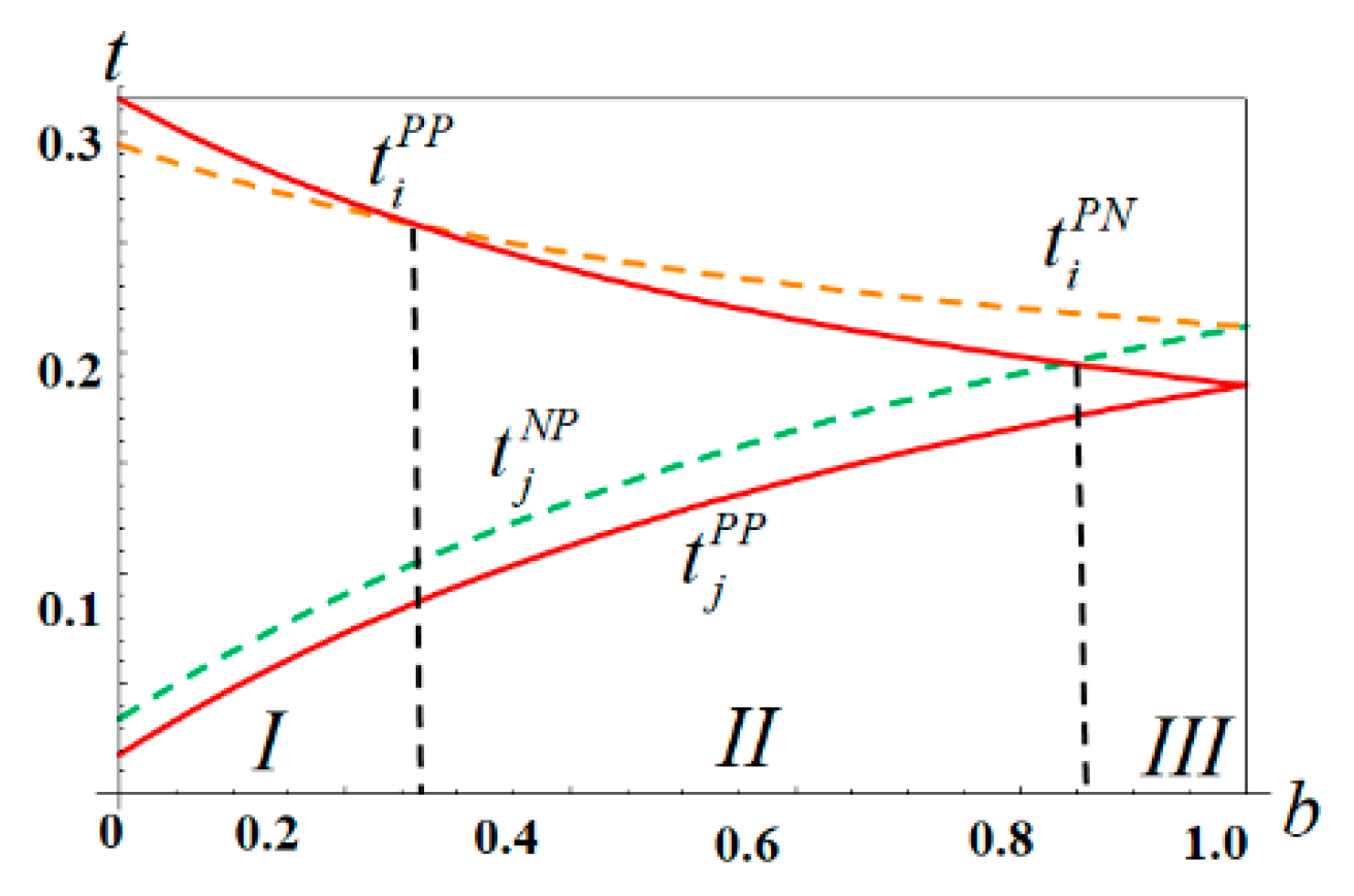
For the comparison of the equilibrium emission taxes under the different policy regimes, we can show an example of the optimal emission taxes in four cases when τ = 0 in Figure 1. In Figure 1, t j N P and t i P N denotes the optimal emission tax in the NP and PN cases, respectively and t i P P and t j P P denotes the optimal emission tax in the PP case.
Proposition 2.
Comparing the optimal emission taxes of the four models provides the following relationships:
(i) 
In Region I, t i P P t i P N > t j N P > t j P P when 0 < b 0.26 ;
(ii) 
In Region II, t i P N > t i P P t j N P > t j P P when 0.26 < b 0.84 and τ 5 < τ < 1 4 ;
(iii) 
In Region III, t i P N > t j N P > t i P P > t j P P when 0.84 < b 1 and 0 τ τ 5 .
Proposition 2 states that the optimal emission tax in each country depends on both the privatization policy and relative market size. The government in the larger country sets the highest emission tax under bilateral privatization or unilateral privatization, while the government in the smaller country always sets the lowest emission tax under bilateral privatization. In particular, t i P P is the highest when 0 < b 0.26 and t i P N is the highest when 0.26 < b 1 in the larger country and t j P P is always lowest when 0 < b 1 . This is because the consumption of the product is always higher in the larger country than in the smaller country, and thus the government in the larger country chooses to impose a higher emission tax to decrease environmental damage. Further, when both governments privatize their ports, the larger country i sets a higher emission tax than that in the smaller country j, that is, t i P P > t j P P . On the contrary, the effect of the privatization policy of the rival country on the emission tax in a larger (smaller) country is dependent (independent) of the relative market size. In particular, port privatization in the smaller country raises the optimal emission tax in the larger country when b is low, that is, t i P P > t i P N when 0 < b < 0.26 ; however, it always decreases the optimal emission tax in the smaller country, that is, t j N P > t j P P .
Proposition 3.
Comparing the equilibrium environmental damage and social welfare of the four models provides the following relationships:
(i) 
E D k N N > E D k P N > E D k N P > E D k P P where k = i , j ;
(ii) 
W i P N > W i N N > W i P P > W i N P   a n d   W j N P > W j N N > W j P N > < W j P P when b < > 0.01 .
Proposition 3 states that the equilibrium environmental damage depends only on the privatization policy. In particular, no privatization yields the highest traffic volume in each country, thus leading to the highest environmental damage. However, bilateral privatization yields the lowest traffic volume in each country, thus leading to the lowest environmental damage. Proposition 3 also states that domestic welfare depends on both the privatization policy and relative market size. First, unilateral privatization leads to the greatest domestic social welfare, that is, W i P N is the highest in country i and W j N P is the highest in country j. Thus, the government has a first-mover advantage to privatize its port to obtain the greatest domestic welfare, which is independent of the relative market size. Second, the two countries prefer no privatization to bilateral privatization regimes, that is, W i N N > W i P P and W j N N > W j P P . Finally, the effect of the port privatization in the larger country on domestic welfare in the smaller country depends on the relative market size. In particular, when the larger country has already privatized its port, the smaller country has an incentive to privatize its port when b is relatively high, that is, W j P N < W j P P when 0.01 < b 1 .

4.2. Privatization Choice Game under Emission Tax

We next consider a privatization choice game between two countries in the first stage, where each country chooses its policy on port ownership simultaneously. 
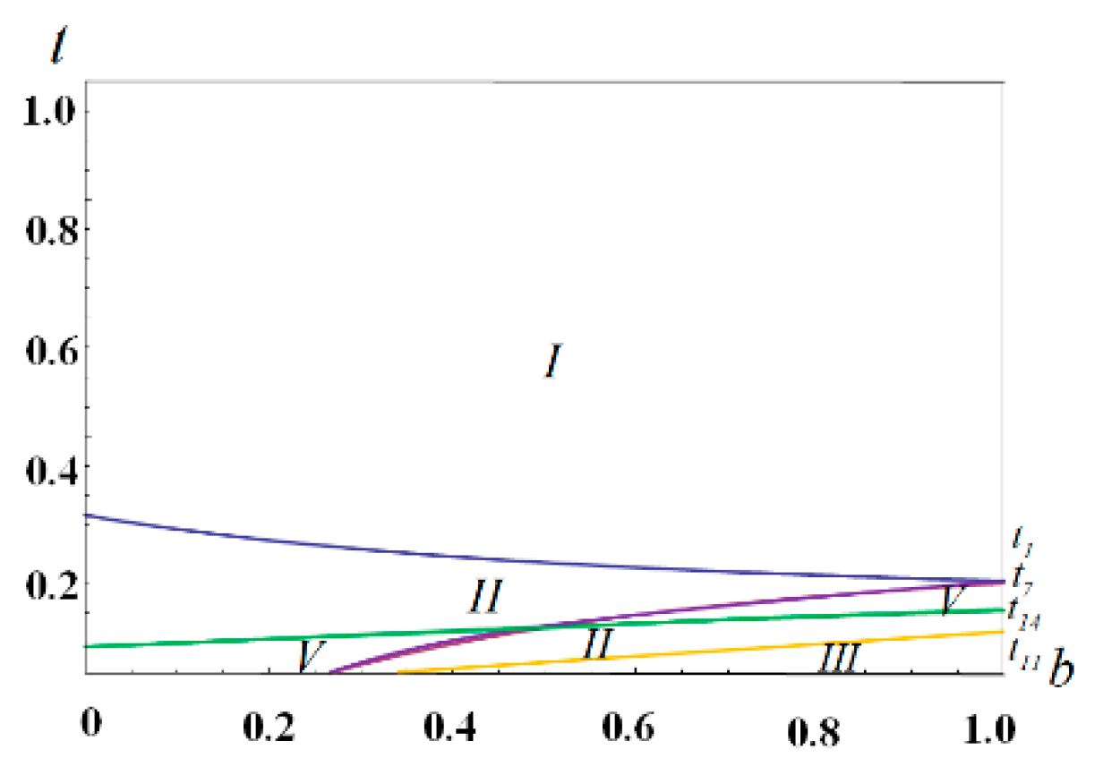
Table 6 shows the payoff matrix of this port privatization choice game. Then, we can obtain the following propositions.
Proposition 4.
In the port privatization choice game under emission tax, we have the following relationships:
(i) 
PN is the unique Nash equilibrium when 0 < b < 0.01 ;
(ii) 
PN and PP are the Nash equilibria when b = 0.01 ;
(iii) 
PP is the unique Nash equilibrium when 0.01 < b 1 .
Proposition 4 states that the Nash equilibrium of this privatization choice game between the two governments depends on the relative market size, while it is independent of the shipping fee. First, the government in the larger country always chooses to privatize its port, while the government in the smaller country chooses to keep its port public if its market size is small enough, that is, 0 < b < 0.01 . Thus, the equilibrium of the port privatization game is a strategic substitute if the b is extremely low. Second, both governments choose to privatize their ports at the equilibrium if the relative market size is large, that is, 0.01 < b 1 . Thus, port privatization policy is a dominant strategy for the government in the larger country, while the smaller country chooses to nationalize (privatize) its port when b is relatively low (high). In particular, the smaller country is more likely to choose to keep its port public when the market size of the rival market is relatively large, and it has a larger incentive to adopt the port privatization policy Thus, the equilibrium of the port privatization game is a strategic complement when the b is relatively high. Finally, the Nash equilibrium is independent of the shipping fee, which sharply contrasts with the finding in Matsushima and Takauchi who did not address environmental concerns under the assumption of exogenous transport cost [26]. However, in our analysis, both countries can utilize the emission tax, which can internalize the transport cost.
To assess the equilibrium outcomes in the privatization choice game, we compare global welfare, which is the sum of the domestic welfare levels, under different policy regimes.
Proposition 5.
The Nash equilibrium in a privatization choice game yields the smallest global welfare unless the smaller country has a sufficiently small market size.
From the viewpoint of global welfare, no privatization policy is the best, while bilateral privatization policy is the worst, i.e., W ¯ N N > W ¯ P N > W ¯ N P > W ¯ P P . Thus, the Nash equilibrium may not be superior from the viewpoint of global welfare. Proposition 5 states that bilateral privatization appears at the equilibrium in a large range of b, that is, 0.01 < b 1 , although no privatization is the best in terms of global welfare. Even though each government could benefit from keeping its port public by expanding the total trade volume, it chooses to privatize its port at the equilibrium because of the rent shift from the foreign country to the domestic country. This result of a competitive privatization policy can be seen as a prisoner’s dilemma under international competition when choosing port privatization policies, which is consistent with the previous result in an international mixed market [38,41].

5. Discussion on Global Emission Taxes

We now consider global concern on the global environment and examine the effects of possible coordination of green policies. Due to climate change in the international economy, there is an imperative global policy discussion on the coordination of environmental policy such as cap-and-trade policy or carbon tax policy in the EU [45,46]. In particular, we examine the coordinated global emission taxes between the two countries and provide policy implications when each government maximizes global welfare instead of its domestic welfare. In the context of the coordinated emission taxes, which are set at the same level t by two governments cooperatively, we can consider two different cases regarding the timing between the global emission taxes and port privatization choices. The first case is that the two governments choose the coordinated emission taxes after the decision of port privatization, while the other is a reversed case that they choose the coordinated emission taxes before the decision of port privatization. Note that the Nash equilibrium is independent of the shipping fee, τ , which is shown in Proposition 4. Thus, we assume that τ = 0 for the convenience of comparisons in the below analysis.

5.1. Global Emission Taxes after Privatization Choices

We first consider the case that two governments choose the coordinated emission taxes after the decision of port privatization. This assumption is supported by the fact that some developing counties have already privatized their ports since the 1970s while the global emission tax is a challenging issue worldwide. Then, we can reexamine the above four cases in Section 3 and obtain the following results, where the superscript * denotes the optimal emission tax after privatization choices under coordination.
Lemma 3.
Comparing the equilibrium global welfare of the four models under coordinated emission taxes after privatization choices provide the following relationships:
(i) 
W ¯ N N * = W ¯ N N , W ¯ N P * > W ¯ N P , W ¯ P N * > W ¯ P N , W ¯ P P * > W ¯ P P ;
(ii) 
W ¯ N N * < W ¯ N P * = W ¯ P N * = W ¯ P P * .
Lemma 3 states that (i) the coordinated emission taxes after privatization choices do not reduce the global welfare and (ii) privatization policy is better than no privatization policy from the view of global welfare. This is because the coordinated emission taxes can eliminate the strategic effects of emission tax from the port privatization policy and thus it can reduce the strategic levels of emission taxes of both countries. Then, the following proposition shows the globally desirable equilibrium under coordinated emission taxes after port privatization choices.
Proposition 6.
Even though bilateral privatization is globally optimal under the coordinated emission taxes after privatization choices, no privatization is the unique Nash equilibrium in the port privatization choice game.
Proposition 6 states that the coordinated emission taxes can induce no privatization policy for both countries, but the equilibrium global welfare is inferior, compared to the bilateral privatization policy. Further, comparing the welfare effect of each country under the coordination of emission taxes in the proof of Lemma 3, we have that W i N N * = W i N N , W j N N * = W j N N , W i P P * < > W i P P when b < > 0.78   and   W j P P * > W j P P . Thus, the coordination of emission taxes can reduce (improve) domestic welfare in the larger (smaller) country in the bilateral privatization policy. This implies that both governments should negotiate the welfare distribution under the coordinated emission taxes after port privatization choices.

5.2. Global Emission Taxes before Privatization Choices

We next consider the other case that two governments choose the coordinated emission taxes before the decision of port privatization. This assumption is also supported by the fact that some other developing counties plan to privatize their ports in the current policy debates of global emission taxes worldwide. We first examine the equilibrium outcomes of the privatization choices game given the specific level of emission taxes, where the superscript “**” denotes the optimal emission tax before privatization choices under coordination.
Lemma 4.
Depending on the emission tax level, all cases among NN, NP, PN and PP could be the Nash equilibrium in the port privatization choice game under the coordinated emission taxes before privatization choices.
Lemma 4 states that two governments can choose any possible equilibrium of the port privatization choice game under the coordinated emission taxes before privatization choices. This is because the coordination before port privatization can fix the privatization race in Proposition 4 where either PP or PN is a unique Nash equilibrium without coordination. When both governments pursue the global welfare-maximization, we will compare the welfare ranks among four cases and find the appropriate level of emission taxes in which Nash equilibrium of the port privatization choice game can be globally desirable.
Proposition 7.
Under the coordinated emission taxes before port privatization choices, no privatization is attainable and globally desirable when the emission tax is high enough.
Proposition 7 implies that if two government agrees on the appropriate emission taxes before port privatization choices, it can induce the greatest global welfare in the equilibrium of the privatization game. In particular, if both countries agree on a higher rate of the coordinated emission tax, the equilibrium of the port privatization game is no privatization, which is globally optimal. Note that the coordination of emission taxes before privatization choices does not affect the global welfare in NN case, while could reduce (improve) the global welfare when the emission tax is relatively low (high) in NP, PN and PP cases, i.e., (i) W ¯ N N * * = W ¯ N N ; (ii) W ¯ N P * * > < W ¯ N P when t < >   t 15 , (iii) W ¯ P N * * > < W ¯ P N when t < > t 16 , (vi) when 0 < b 0.63 , W ¯ P P * * > < W ¯ P P when t < > t 17 ; when 0.63 < b 1 , W ¯ P P * * > W ¯ P P when t 18 < t < t 17 , otherwise, W ¯ P P * * < W ¯ P P . It also states that the globally desirable equilibrium of the privatization choice game depends on the emission tax level, while it is independent of the relative market size. This finding provides an important global policy implication in the coordination of emission taxes before port privatization choices game. In particular, if both countries agree on the coordinated emission taxes, it will be helpful not only to reduce global welfare loss from the privatization race, but to include global concern on climate change before industrial policies and emission strategies among the countries are determined. Therefore, environmental policy coordination between the governments for global welfare is imperatively required in the port privatization policies.

6. Conclusions

This study considered strategic port privatization and emission tax policies under international competition and found that the equilibrium outcomes depend critically on the relative market size between the two countries. We showed that as a substitute for port privatization policy, the emission tax can be higher than marginal environmental damage in the larger country, while it may be lower (higher) than marginal environmental damage when the relative market size is (not so) small in the smaller country. We also showed that there may be excessive initiatives in the competitive race of privatization policy choices where port privatization policy is a dominant strategy for the larger country while the smaller country chooses to nationalize (privatize) its port when its market size is relatively (not so) small. Thus, the equilibrium in a privatization policy game may yield the smallest global welfare. Finally, we investigated the coordinated global emission taxes and compared the effects on the port privatization choices game. We showed that the global emission taxes before privatization choices can induce the equilibrium of the game to be globally optimal when the global emission tax is relatively high. This finding provides an important global policy implication on the climate change that coordinated environmental policy between the countries is imperatively required in the port privatization policies.
There remain the limitations of the study. First, we could not incorporate the effects of practical market factors such as product differentiation, the number of firms in different market structures, competition within the ports, between terminals or with other port terminals. We also used linear demand and quadratic cost functions for tractability, but the generalization of the model specifications is imperative for further policy implications. For instance, a situation in which multiple ports compete in an area under multiple regime scenarios is more common and quite interesting. Finally, but not least, some important policy instruments such as partial privatization or/and tariff policies should be further examined for a better understanding of the results. These extensions remain as future research.

Author Contributions

Conceptualization, S.-H.L. and L.X.; methodology, L.X.; software, F.P. and L.X.; validation, F.P., L.X. and Y.C.; formal analysis, L.X. and S.-H.L.; investigation, F.P.; resources, F.P.; data curation, Y.C.; writing—original draft preparation, L.X.; writing—review and editing, F.P., L.X. and S.-H.L.; visualization, F.P.; supervision, L.X.; project administration, S.-H.L.; funding acquisition, F.P. All authors have read and agreed to the published version of the manuscript.

Funding

This research was funded by the Youth Program of National Natural Science Foundation of China, grand number 41701134 and the Postdoctoral Science Foundation of China, grand number 2019M651098.

Acknowledgments

We thank three anonymous referees for their careful and constructive comments on an earlier version of this paper. All remaining errors are ours.

Conflicts of Interest

The authors declare no conflict of interest.

Appendix A

The Value of A i , τ i , and t i
A 1 = ( 5 τ ) ( 1 + τ ) ( 1 2 τ ) 2 b 2 ,
A 2 = ( 1 2 τ ) 2 + b ( 2 τ ) ( 2 + 5 τ ) b 2 ( 1 2 τ ) 2 ,
A 3 = 274 + 529 b + 383 b 2 + 124 b 3 + 16 b 4 2 ( 1 + b ) ( 1 + 2 b ) ( 13 + 12 b + 4 b 2 ) τ + 4 ( 1 + b ) 2 ( 13 + 12 b + 4 b 2 ) τ 2 ,
A 4 = 4 + 279 b + 507 b 2 + 340 b 3 + 100 b 4 + 12 b 5 32 τ 72 b τ 24 b 2 τ + 40 b 3 τ + 24 b 4 τ + 64 τ 2 + 156 b τ 2 + 104 b 2 τ 2 4 b 3 τ 2 16 b 4 τ 2 ,
A 5 = 441 + 1180 b + 1296 b 2 + 676 b 3 + 144 b 4 ,
A 6 = 4 + 449 b + 1180 b 2 + 1288 b 3 + 672 b 4 + 144 b 5 ,
A 7 = 1465 + 3866 b + 4148 b 2 + 2108 b 3 + 436 b 4 ,
A 8 = 144 + 476 b + 476 b 2 + 135 b 3 + 11 b 4 16 τ 40 b τ 24 b 2 τ + 8 b 3 τ + 8 b 4 τ + 44 τ 2 + 136 b τ 2 + 124 b 2 τ 2 + 16 b 3 τ 2 16 b 4 τ 2 ,
A 9 = 8 + 172 b + 506 b 2 + 489 b 3 + 139 b 4 + 12 b 5 32 τ 116 b τ 134 b 2 τ 58 b 3 τ 8 b 4 τ + 32 τ 2 + 132 b τ 2 + 184 b 2 τ 2 + 100 b 3 τ 2 + 16 b 4 τ 2 ,
A 10 = b ( 1060 + 1481 b + 796 b 2 + 144 b 3 ) + 8 b ( 45 + 37 b + 8 b 2 ) τ ,
A 11 = 4 + b ( 264 + 1060 b + 1473 b 2 + 792 b 3 + 144 b 4 ) ,
A 12 = 8 + 900 b + 3514 b 2 + 4717 b 3 + 2452 b 4 + 432 b 5 ,
A 13 = 59 + 3 b ( 1 2 τ ) 2 b 2 ( 1 2 τ ) 2 ( 2 11 τ ) τ ( 25 + 24 b + 4 b 2 ) t i 2 ,
A 14 = 4 ( 1 2 τ ) 2 ( 4 b 2 ) + b ( 58 + 2 τ + 7 τ 2 ) + ( 16 + 7 b 4 b 2 ) t i 2 ,
A 15 = 87 + 91 b + 24 b 2 21 τ 8 b τ + 42 τ 2 + 16 b τ 2 ,
A 16 = 1487 + 5391 b + 8068 b 2 + 6268 b 3 + 2536 b 4 + 432 b 5 280 τ 888 b τ 1064 b 2 τ 584 b 3 τ 128 b 4 τ + 560 τ 2 + 1776 b τ 2 + 2128 b 2 τ 2 + 1168 b 3 τ 2 + 256 b 4 τ 2 ,
A 17 = 892 + 4436 b + 8303 b 2 + 7223 b 3 + 2896 b 4 + 432 b 5 200 τ 808 b τ 1144 b 2 τ 664 b 3 τ 128 b 4 τ + 400 τ 2 + 1616 b τ 2 + 2288 b 2 τ 2 + 1328 b 3 τ 2 + 256 b 4 τ 2 ,
τ 1 = 10 + 3 b + 16 b 2 + 8 b 3 2 ( 1 + b ) ( 2 + 11 b + 4 b 2 ) , τ 2 = 1 4 3 ( 1 b ) ( 22 + 29 b + 12 b 2 ) 4 ( 1 + b ) ( 1 b ) ( 1 + b ) ( 9 + 8 b ) ,
τ 3 = 1 24 b 36 b 2 16 b 3 4 ( 1 + b ) 2 ( 1 4 b ) , τ 4 = 1 15 b 4 b 2 2 ( 2 3 b ) ,
τ 5 = 667 + 298 b 682 b 2 640 b 3 112 b 4 4 ( 73 67 b 279 b 2 180 b 3 16 b 4 ) ,
t 1 = 4 + 2 b + b 2 ( 1 + b ) ( 15 + 8 b ) , t 2 = 164 + 540 b + 583 b 2 + 252 b 3 + 40 b 4 2 ( 1 + b ) ( 15 + 8 b ) ( 17 + 34 b + 12 b 2 ) ,
t 3 = 5 + 2 b 2 2 ( 10 + 9 b + 4 b 2 ) , t 4 = 179 + 282 b + 178 b 2 + 48 b 3 + 8 b 4 2 ( 358 + 681 b + 464 b 2 + 132 b 3 + 16 b 4 ) ,
t 5 = 1 + 5 b + 3 b 2 ( 1 + b ) ( 15 + 8 b ) , t 6 = 89 + 402 b + 610 b 2 + 390 b 3 + 88 b 4 2 ( 1 + b ) ( 15 + 8 b ) ( 22 + 29 b + 12 b 2 ) .
t 7 = 2 + 7 b + 2 b 2 2 ( 5 + 14 b + 4 b 2 ) , t 8 = 68 + 244 b + 289 b 2 + 86 b 3 + 8 b 4 2 ( 208 + 641 b + 614 b 2 + 172 b 3 + 16 b 4 ) ,
t 9 = 3 + 4 b 2 ( 15 + 8 b ) , t 10 = 27 + 60 b + 32 b 2 2 ( 135 + 192 b + 64 b 2 ) ,
t 11 = 16 2 b + 110 b 2 + 97 b 3 + 16 b 4 ( 1 + b ) 2 ( 297 + 336 b + 64 b 2 ) , t 12 = 5 + 2 b 2 2 ( 10 + 9 b + 4 b 2 ) ,
t 13 = 45 + 112 b + 126 b 2 + 16 b 3 2 ( 252 + 467 b + 252 b 2 + 32 b 3 ) , t 14 = 18 + 65 b + 110 b 2 + 16 b 3 414 + 944 b + 584 b 2 + 64 b 3 ,
t 15 = 3 + 36 b + 48 b 2 + 20 b 3 88 + 204 b + 164 b 2 + 48 b 3 , t 16 = 20 + 48 b + 31 b 2 + 8 b 3 68 + 204 b + 184 b 2 + 48 b 3 ,
t 17 = 9 + 4 b 2 ( 27 + 8 b ) , t 18 = 81 + 108 b + 32 b 2 2 ( 243 + 288 b + 64 b 2 ) .

Appendix B

The Proof of Propositions and Lemmas
Proof of Proposition 1.
(i)
p i P P p i N P = ( 5 + 6 b 4 b 2 ) ( 1 4 τ ) 2 ( 27 + 8 b ) ( 22 + 29 b + 12 b 2 ) > 0 ,
p i N P p i P N = 5 ( 1 b 2 ) ( 1 4 τ ) 2 ( 22 + 29 b + 12 b 2 ) ( 17 + 34 b + 12 b 2 ) > 0 ,
p i P N p i N N = ( 2 + 11 b + 4 b 2 ) ( 1 4 τ ) 2 ( 15 + 8 b ) ( 17 + 34 b + 12 b 2 ) > 0 ,
(ii)
f i P N f i P P = ( 22 + 128 b + 251 b 2 + 136 b 3 + 16 b 4 ) ( 1 4 τ ) 4 ( 1 + b ) ( 27 + 8 b ) ( 17 + 34 b + 12 b 2 ) > 0 ,
f i P P f i N N = 3 ( 1 + 11 b ) ( 1 4 τ ) 2 ( 1 + b ) ( 15 + 8 b ) ( 27 + 8 b ) > 0 ,
f i N N f i N P = ( 7 + 6 b + 4 b 2 ) 2 ( 1 4 τ ) 4 ( 1 + b ) ( 15 + 8 b ) ( 22 + 29 b + 12 b 2 ) > 0 ,
f j N P f j P P = ( 67 + 168 b + 206 b 2 + 96 b 3 + 16 b 4 ) ( 1 4 τ ) 4 ( 1 + b ) ( 27 + 8 b ) ( 22 + 29 b + 12 b 2 ) > 0 ,
f j P P f j N N = 3 ( 11 + b ) ( 1 4 τ ) 2 ( 1 + b ) ( 15 + 8 b ) ( 27 + 8 b ) > 0 ,
f j N N f j P N = ( 2 + 11 b + 4 b 2 ) 2 ( 1 4 τ ) 4 ( 1 + b ) ( 15 + 8 b ) ( 17 + 34 b + 12 b 2 ) > 0 . □
Proof of Proposition 2.
(i)
t i P P t i P N = ( 38 62 b 269 b 2 160 b 3 16 b 4 ) ( 1 4 τ ) 4 ( 1 + b ) ( 27 + 8 b ) ( 17 + 34 b + 12 b 2 ) > < 0 when b < > 0.26 ,
(ii)
t i P N t j N P = 389 + 922 b + 238 b 2 753 b 3 652 b 4 144 b 5 60 τ 220 b τ 100 b 2 τ + 220 b 3 τ + 160 b 4 τ 4 ( 1 + b ) ( 22 + 29 b + 12 b 2 ) ( 17 + 34 b + 12 b 2 ) > 0 ,
(iii)
t i P P t j N P = 667 + 298 b 682 b 2 640 b 3 112 b 4 292 τ + 268 b τ + 1116 b 2 τ + 720 b 3 τ + 64 b 4 τ 4 ( 1 + b ) ( 27 + 8 b ) ( 22 + 29 b + 12 b 2 ) 0 if 0.84 < b 1 and 0 τ τ 5 . Otherwise, t i P P > t j N P ,
(iv)
t j N P t j P P = ( 37 + 102 b + 194 b 2 + 120 b 3 + 16 b 4 ) ( 1 4 τ ) 4 ( 1 + b ) ( 27 + 8 b ) ( 22 + 29 b + 12 b 2 ) > 0 ,
(v)
t i P P t j P P = ( 1 b ) ( 8 + 2 b 5 τ ) ( 1 + b ) ( 27 + 8 b ) > 0 . □
Proof of Proposition 3.
(i)
E D i N N E D i P N = ( 1 + b ) 2 ( 2 + 11 b + 4 b 2 ) ( 32 + 57 b + 20 b 2 ) ( 1 4 τ ) 2 2 ( 15 + 8 b ) 2 ( 17 + 34 b + 12 b 2 ) 2 > 0 ,
E D i P N E D i N P = 15 ( 1 b ) ( 1 + b ) 5 ( 13 + 8 b ) ( 1 4 τ ) 2 2 ( 22 + 29 b + 12 b 2 ) 2 ( 17 + 34 b + 12 b 2 ) 2 > 0 ,
E D i N P E D i P P = ( 1 + b ) 2 ( 5 + 6 b 4 b 2 ) ( 49 + 64 b + 20 b 2 ) ( 1 4 τ ) 2 2 ( 27 + 8 b ) 2 ( 22 + 29 b + 12 b 2 ) 2 > 0 ,
(ii)
W i P N W i N N = ( 2 + 11 b + 4 b 2 ) 2 ( 1 4 τ ) 2 8 ( 15 + 8 b ) 2 ( 17 + 34 b + 12 b 2 ) > 0 ,
W i N N W i P P = 3 ( 321 + 247 b + 56 b 2 ) ( 1 4 τ ) 2 2 ( 15 + 8 b ) 2 ( 27 + 8 b ) 2 > 0 ,
W i P P W i N P = ( 2623 + 10198 b + 19648 b 2 + 20636 b 3 + 11600 b 4 + 3232 b 5 + 320 b 6 ) ( 1 4 τ ) 2 8 ( 27 + 8 b ) 2 ( 22 + 29 b + 12 b 2 ) 2 > 0 ,
(iii)
W j N P W j N N = ( 7 + 6 b + 4 b 2 ) 2 ( 1 4 τ ) 2 8 ( 15 + 8 b ) 2 ( 22 + 29 b + 12 b 2 ) > 0 ,
W j N N W j P N = ( 2 + 11 b + 4 b 2 ) ( 8 + 17 b + 4 b 2 ) ( 32 + 57 b + 20 b 2 ) ( 1 4 τ ) 2 8 ( 15 + 8 b ) 2 ( 17 + 34 b + 12 b 2 ) 2 > 0 ,
W j N N W j P P = 3 ( 111 + 377 b + 136 b 2 ) ( 1 4 τ ) 2 2 ( 15 + 8 b ) 2 ( 27 + 8 b ) 2 > 0 ,
W j P N W j P P = ( 52 3988 b 17658 b 2 26091 b 3 16140 b 4 4112 b 5 320 b 6 ) ( 1 4 τ ) 2 8 ( 27 + 8 b ) 2 ( 17 + 34 b + 12 b 2 ) 2 > < 0 if b < > 0.01 . □
Proof of Proposition 4.
When 0 τ < 1 4 , we have W i N N < W i P N , W i N P < W i P P , W j N N < W j N P , and W j P N > < W j P P if b < > 0.01 . □
Proof of Proposition 5.
The global welfares in the four cases are: W ¯ N N = ( 1 + b ) A 15 ( 15 + 8 b ) 2 , W ¯ P N = A 16 8 ( 22 + 29 b + 12 b 2 ) 2 , W ¯ N P = A 17 8 ( 17 + 34 b + 12 b 2 ) 2 , and W ¯ P P = ( 1 + b ) ( 279 + 163 b + 24 b 2 45 τ 8 b τ + 90 τ 2 + 16 b τ 2 ) ( 27 + 8 b ) 2 , respectively. Comparing these results, we have the following relationships:
(i)
W ¯ N N W ¯ P N = ( 1 + b ) ( 2 + 11 b + 4 b 2 ) ( 222 + 523 b + 268 b 2 + 32 b 3 ) ( 1 4 τ ) 2 8 ( 15 + 8 b ) 2 ( 17 + 34 b + 12 b 2 ) 2 > 0 ,
(ii)
W ¯ P N W ¯ N P = 5 ( 1 b ) ( 1 + b ) 2 ( 397 + 1252 b + 1309 b 2 + 600 b 3 + 96 b 4 ) ( 1 4 τ ) 2 8 ( 22 + 29 b + 12 b 2 ) 2 ( 17 + 34 b + 12 b 2 ) 2 > 0 ,
(iii)
W ¯ N P W ¯ P P = ( 1 + b ) ( 5 + 6 b 4 b 2 ) ( 747 + 950 b + 420 b 2 + 32 b 3 ) ( 1 4 τ ) 2 8 ( 27 + 8 b ) 2 ( 22 + 29 b + 12 b 2 ) 2 > 0 . □
Proof of Proposition 6.
(i)
W ¯ N P * W ¯ N N * = 9 ( 1 + b ) ( 1 4 τ ) 2 2 ( 9 + 8 b ) ( 15 + 8 b ) 2 > 0 ,
(ii)
W ¯ N P * = W ¯ P N * = W ¯ P P * = ( 1 + b ) ( 7 + 6 b 2 τ + 4 τ 2 ) 2 ( 9 + 8 b ) ,
(iii)
W i N P * W i N N * = W j N N * W j N P * = 6 ( 3 + 2 b ) ( 13 + 4 b ( 3 + b ) ) ( 1 4 τ ) 2 ( 9 + 8 b ) 2 ( 15 + 8 b ) 2 > 0 ,
(iv)
W i N N * W i P N * = W j P N * W j N N * = ( 1 4 τ ) ( 657 + 456 b 562 b 2 576 b 3 128 b 4 603 τ + 111 b τ + 784 b 2 τ + 320 b 3 τ ) 2 ( 9 + 8 b ) 2 ( 15 + 8 b ) 2 > 0 ,
(v)
W i P N * W i P P * = W j P P * W j P N * = ( 1 4 τ ) ( 2 3 b 2 b 2 + τ + 11 b τ ) 2 ( 9 + 8 b ) 2 > < 0 if b < >   3 + 11 τ + 25 58 τ + 121 τ 2 4 . □
Proof of Proposition 7.
First, we compare the global welfare ranks among the four cases.
(i)
W ¯ N N * * W ¯ N P * * = 2 ( 1 + b ) ( 1 5 b 3 b 2 + ( 1 + b ) ( 15 + 8 b ) t ) ( 66 + 135 t + b ( 17 + 327 t + b ( 55 24 b + 64 ( 4 + b ) t ) ) ) ( 15 + 8 b ) 2 ( 19 + 2 b ( 9 + 2 b ) ) 2 . Thus, we have:
(i-1) if 0 < b 0.180 , W ¯ N N * * > W ¯ N P * * ;
(i-2) if 0.180 < b 1 , W ¯ N N * * < W ¯ N P * * when 0 < t < t 5 , and W ¯ N N * * W ¯ N P * * when t 5 < t 1 .
(ii)
W ¯ N N * * W ¯ P N * * = 2 ( 1 + b ) ( 4 2 b b 2 + ( 1 + b ) ( 15 + 8 b ) t ) ( 6 + 135 t + b ( 19 + 327 t + b ( 13 8 b + 64 ( 4 + b ) t ) ) ) ( 15 + 8 b ) 2 ( 14 + b ( 23 + 4 b ) ) 2 . Thus, we have that W ¯ N N * * < W ¯ P N * * when 0 < t < t 6 , and W ¯ N N * * W ¯ P N * * when t 6 t 1 .
(iii)
W ¯ N N * * W ¯ P P * * = ( 1 + b ) ( 3 + 30 t + 4 b ( 1 + 4 t ) ) ( 27 + 270 t + 4 b ( 15 8 b + 32 ( 3 + b ) t ) ) 162 ( 15 + 8 b ) 2 . Thus, we have:
(iii-1) if 0 < b 0.375 , W ¯ N N * * < W ¯ P P * * when 0 < t < t 9 and W ¯ N N * * W ¯ P P * * when t 9 t 1 ;
(iii-2) if 0.375 < b 1 , W ¯ N N * * < W ¯ P P * * when 0 < t 10 < t < t 9 ; otherwise, W ¯ N N * * W ¯ P P * * .
(iv)
W ¯ N P * * W ¯ P N * * = 2 ( 1 + b ) ( 1 + b ) 2 ( 6 + b 5 t ) ( 16 + 2 b 110 b 2 97 b 3 16 b 4 + ( 1 + b ) 2 ( 9 + 8 b ) ( 33 + 8 b ) t ) ( 19 + 2 b ( 9 + 2 b ) ) 2 ( 14 + b ( 23 + 4 b ) ) 2 . Thus, we have:
(iv-1) if 0 < b 0.339 , W ¯ N P * * < W ¯ P N * * ;
(iv-2) if 0.339 < b 1 , W ¯ N P * * > W ¯ P N * * when 0 < t < t 11 ; W ¯ N P * * W ¯ P N * * when t 11 t 1 .
(v)
W ¯ N P * * W ¯ P P * * = ( 1 + b ) ( 5 + 20 t + 18 b t + b 2 ( 2 + 8 t ) ) ( 9 ( 5 + 56 t ) + 2 b ( 56 + 467 t + b ( 63 + 8 b ) ( 1 + 4 t ) ) ) 162 ( 19 + 2 b ( 9 + 2 b ) ) 2 . Thus, we have:
( v -1) if 0 < b 0.298 , W ¯ N P * * < W ¯ P P * * when 0 < t < t 12 , and W ¯ N P * * W ¯ P P * * when t 12 t 1 ;
(v-2) if 0.298 < b 1 , W ¯ N P * * < W ¯ P P * * when 0 < t 13 < t < t 12 ; otherwise, W ¯ N P * * W ¯ P P * * .
(vi)
W ¯ P N * * W ¯ P P * * = ( 1 + b ) ( 2 + 10 t + b ( 7 + 2 b ) ( 1 + 4 t ) ) ( 18 + 414 t + b ( 65 + 944 t + 2 b ( 55 8 b + 4 ( 73 + 8 b ) t ) ) ) 162 ( 14 + b ( 23 + 4 b ) ) 2 . Thus, we have:
(vi-1) if 0 < b 0.266 , W ¯ P N * * < W ¯ P P * * when 0 < t < t 14 , and W ¯ P N * * W ¯ P P * * when t 14 t 1 ;
(vi-2) if 0.266 < b < 0.5 , W ¯ P N * * < W ¯ P P * * when 0 < t 7 < t < t 14 ; otherwise, W ¯ P N * * W ¯ P P * * ;
(iv-3) if b = 0.5 , W ¯ P N * * W ¯ P P * * ;
(iv-4) if 0.5 < b 1 , W ¯ P N * * < W ¯ P P * * when t 14 < t < t 7 ; otherwise, W ¯ P N * * W ¯ P P * * .
The following Figure A1 shows the maximized global welfare under coordinated emission taxes before privatization choices.
Figure A1. Maximized global welfare under coordinated emission taxes before privatization ( τ = 0 ) .
Sustainability 12 06595 g0a1
Then, from Figure A1, we obtain the following conditions:
(i)
In Regain I, W ¯ N N * * is highest when t 1 t 1 ;
(ii)
In Regain II, W ¯ P N * * is highest when max { t 14 , t 7 } t t 6 ; and max { 0 , t 11 } t min { t 14 , t 7 } if 0.266 < b 1 ;
(iii)
In Regain III, W ¯ N P * * is highest when 0 t t 11 ;
(iv)
In Regain V, W ¯ P P * * is highest when 0 t t 14 and t 7 < 0 ; min { t 14 , t 7 } t max { t 14 , t 7 } if t 7 > 0 . □
Proof of Lemma 1.
(i)
Q i N N > Q j N N , Q i N P > Q j N P , Q i P N > Q j P N , Q i P P > Q j P P ,
(ii)
π i N N > π j N N , π i N P > π j N P , π i P N > π j P N , π i P P > π j P P ,
(iii)
W i N N > W j N N , W i N P > W j N P , W i P N > W j P N , W i P P > W j P P . □
Proof of Lemma 2.
(i)
t i P N M E D i P N = 16 + 36 b + 19 b 2 + 4 b 3 + 4 τ 8 b τ 28 b 2 τ 16 b 3 τ 4 ( 1 + b ) ( 17 + 34 b + 12 b 2 ) > 0 ,
(ii)
t i P P M E D i P P = 15 + 3 b 6 τ + 4 b τ 54 + 70 b + 16 b 2 > 0 ,
(iii)
t j N P M E D j N P = 1 + 24 b + 36 b 2 + 16 b 3 + 4 τ 8 b τ 28 b 2 τ 16 b 3 τ 4 ( 1 + b ) ( 22 + 29 b + 12 b 2 ) 0 if 0 < b < 0.04 and 0 τ τ 3 . Otherwise, t j N P > M E D j N P ,
(iv)
t j P P M E D j P P = 1 + 15 b + 4 b 2 + 4 τ 6 b τ 2 ( 1 + b ) ( 27 + 8 b ) 0 if 0 < b < 0.07 and 0 τ τ 4 . Otherwise, t j P P > M E D j P P . □
Proof of Lemma 3.
(i)
NN case: The coordination of emission taxes does not affect the equilibrium outcomes because the emission tax policy is independent of domestic welfare when the two governments keep their port public. Thus, domestic welfare under the coordination of emission taxes is the same as that in Table 1, that is, W i N N * = W i N N and W j N N * = W j N N . Thus, W ¯ N N * = W ¯ N N .
(ii)
NP case: We substitute t = t i = t j into Equation (10) when both governments set the same emission taxes. The differentiation of the sum of domestic welfare in Equation (10) with respect to t yields the following coordinated emission tax: t N P * = 5 + 4 b + 6 b 2 2 ( 1 + b ) ( 9 + 8 b ) < > 0 when b < > 0.40 . The resulting domestic welfare and global welfare are W i N P * = 64 + 111 b + 49 b 2 2 ( 9 + 8 b ) 2 , W j N P * = 62 b + 109 b 2 + 48 b 3 1 2 ( 9 + 8 b ) 2 , and W ¯ N P * = 7 + 13 b + 6 b 2 2 ( 9 + 8 b ) . Thus, W i N P * > W i N P , W j N P * < W j N P and W ¯ N P * > W ¯ N P .
(iii)
PN case: The differentiation of the sum of domestic welfare in Equation (14) with respect to t yields t P N * = 2 + b + 2 b 2 2 ( 1 + b ) ( 9 + 8 b ) . The resulting welfares are W i P N * = 61 + 108 b + 49 b 2 2 ( 9 + 18 b ) 2 , W j P N * = 2 + 65 b + 109 b 2 + 48 b 3 2 ( 9 + 18 b ) 2 , and W ¯ P N * = 7 + 13 b + 6 b 2 2 ( 9 + 8 b ) . Thus, W i P N * < W i P N , W j P N * > W j P N and W ¯ P N * > W ¯ P N .
(iv)
PP case: The differentiation of the sum of domestic welfare in Equation (17) with respect to t yields t P P * = 4 b 2 ( 9 + 8 b ) . The resulting welfares are   W i P P * = 59 + 111 b + 51 b 2 2 ( 9 + 8 b ) 2 , W j P P * = 4 + 62 b + 107 b 2 + 48 b 3 2 ( 9 + 8 b ) 2 , and W ¯ P P * = 7 + 13 b + 6 b 2 2 ( 9 + 8 b ) . Thus, W i P P * < > W i P P when b < > 0.78 , W j P P * > W j P P and W ¯ P P * > W ¯ P P . □
Proof of Lemma 4.
First, we compare the welfare ranks among the possible scenarios.
(i)
W i N N * * W i P N * * = ( 4 2 b b 2 + ( 1 + b ) ( 15 + 8 b ) t ) ( 164 540 b 583 b 2 252 b 3 40 b 4 + 2 ( 1 + b ) ( 15 + 8 b ) ( 17 + 2 b ( 17 + 6 b ) ) t ) ( 15 + 8 b ) 2 ( 14 + b ( 23 + 4 b ) ) 2 . Then, W i N N * * < W i P N * * if t 1 < t < t 2 ; otherwise, W i N N * * W i P N * * , where t i (i =1,…, 18) is as presented in Appendix A.
(ii)
W i N P * * W i P P * * = ( 5 + 20 t + 18 b t + b 2 ( 2 + 8 t ) ) ( 179 ( 1 + 4 t ) + 2 b ( 141 b ( 89 + 4 b ( 6 + b ) ) + ( 681 + 4 b ( 116 + b ( 33 + 4 b ) ) ) t ) ) 162 ( 19 + 2 b ( 9 + 2 b ) ) 2 . Then, W i N P * * < W i P P * * if t 3 < t < t 4 ; otherwise W i N P * * W i P P * * .
(iii)
W j N N * * W j N P * * = ( 1 5 b 3 b 2 + ( 1 + b ) ( 15 + 8 b ) t ) ( 89 402 b 610 b 2 390 b 3 88 b 4 + 2 ( 1 + b ) ( 15 + 8 b ) ( 22 + b ( 29 + 12 b ) ) t ) ( 15 + 8 b ) 2 ( 19 + 2 b ( 9 + 2 b ) ) 2 . Then, we have the following relationships:
(iii-1) if 0 < b 0.180 , W j N N * * < W j N P * * when 0 < t < t 6 , and W j N N * * W j N P * * when t 6 t < 1 ;
(iii-2) if 0.180 < b 1 , W j N N * * < W j N P * * when 0 < t 5 < t < t 6 ; otherwise, W j N N * * W j N P * * .
(iv)
W j P N * * W j P P * * = ( 2 + 10 t + b ( 7 + 2 b ) ( 1 + 4 t ) ) ( 68 + 416 t + b ( 244 + 1282 t + b ( 289 + 1228 t + 2 b ( 43 + 4 b ) ( 1 + 4 t ) ) ) ) 162 ( 14 + b ( 23 + 4 b ) ) 2 . Then, we have the following relationships:
(iv-1) if 0 < b 0.266 , W j P N * * < W j P P * * when 0 < t < t 8 , and W j P N * * W j P P * * when t 8 t < 1 ;
(iv-2) if 0.266 < b 1 , W j P N * * < W j P P * * when 0 < t 7 < t < t 8 ; otherwise, W j P N * * W j P P * * .
Then, we show that the Nash equilibrium in the privatization choice game under the coordinated emission taxes before privatization choices are as follows:
(i)
NN is a Nash equilibrium if one of the following conditions are met: (i-1) t ( t 2 ,1) for all b; (i-2) t ( 0 , t 5 ) and b ( 0.180 ,   1 ] ; (i-3) t ( t 6 , t 1 ) and b ( 0 ,   0.354 ] .
(ii)
PN is a Nash equilibrium if one of the following conditions are met: (ii-1) t ( t 1 , t 2 ) and b [ 0 , 0.432 , 1 ) ; (ii-2) t ( t 8 , t 2 ) and b ( 0.432 , 1 ] .
(iii)
NP is a Nash equilibrium if one of the following conditions are met: (iii-1)   t ( 0 , t 6 ) and b ( 0 , 0.180 ] ; (iii-2) t ( t 5 ,   t 6 ) and b ( 0.180 , 0.323 ] ; (iii-3) t ( t 5 , t 3 ) and b ( 0.323 , 1 ] ; (iii-4) t ( t 4 ,   t 6 ). if b ( 0.514 , 1 ]
(iv)
PP is a Nash equilibrium if t ( t 3 , t 8 ) and b ( 0.383 , 1 ] . □

References

  1. World Bank. Port Reform Toolkit, Module 3: Alternative Port Management Structures and Ownership Models; The World Bank: Washington, DC, USA, 2007; Available online: https://ppiaf.org/sites/ppiaf.org/files/documents/toolkits/Portoolkit/Toolkit/pdf/modules/03_TOOLKIT_Module3.pdf (accessed on 22 October 2006).
  2. Midoro, R.; Musso, E.; Parola, F. Maritime liner shipping and the stevedoring industry: Market structure and competition strategies. Mar. Policy Manag. 2005, 32, 89–106. [Google Scholar] [CrossRef]
  3. Gong, S.X.; Cullinanne, K.; Firth, M. The impact of airport and seaport privatization on efficiency and performance: A review of the international evidence and implications for developing countries. Transp. Policy 2012, 24, 37–47. [Google Scholar] [CrossRef]
  4. Czerny, A.; Höffler, F.; Mun, S.I. Hub port competition and welfare effect of strategic privatization. Econ. Transp. 2014, 3, 211–220. [Google Scholar] [CrossRef] [Green Version]
  5. Hong Kong Environmental Protection Department. Hong Kong Air Pollutant Emission Inventory; The Government of Hong Kong: Hong Kong, China, 2017. Available online: https://www.epd.gov.hk/epd/english/environmentinhk/air/data/emission_inve_navigation.html (accessed on 18 June 2019).
  6. International Maritime Organization. Third IMO GHG Study 2014; International Maritime Organization: London, UK, 2014; Available online: http://www.imo.org/en/OurWork/Environment/PollutionPrevention/AirPollution/Pages/Greenhouse-Gas-Studies-2014.aspx (accessed on 13 October 2014).
  7. Baltazar, R.; Brooks, M.R. The Governance of Port Devolution: A Tale of Two Countries. In Proceedings of the 9th World Congress on Transport Research, Seoul, Korea, 22–27 July 2001. [Google Scholar]
  8. Czerny, A.I. Public versus private airport behavior when concession revenues exist. Econ. Transp. 2013, 2, 38–46. [Google Scholar] [CrossRef] [Green Version]
  9. Liu, Z. The comparative performance of public and private enterprises: The case of British ports. J. Transp. Econ. Policy 1995, 29, 263–274. [Google Scholar]
  10. Trujillo, L.; Nombela, G. Privatization and Regulation of the Seaport Industry; The World Bank: Washington, DC, USA, 1999. [Google Scholar]
  11. Notteboom, T.; Coeck, C.; Julien, V.D.B. Measuring and explaining the relative efficiency of container terminals by means of Bayesian stochastic frontier models. Int. J. Mar. Econ. 2000, 2, 83–106. [Google Scholar] [CrossRef]
  12. Estache, A.; Gonzalez, M.; Trujillo, L. Efficiency gains from port reform and the potential for yardstick competition: Lessons from Mexico. World Dev. 2002, 30, 545–560. [Google Scholar] [CrossRef]
  13. Barros, C.P.; Athanassiou, M. Efficiency in European seaports with DEA: Evidence from Greece and Portugal. Mar. Econ. Logist. 2004, 6, 122–140. [Google Scholar] [CrossRef]
  14. Cheon, S.H.; Dowall, D.E.; Song, D.W. Evaluating impacts of institutional reforms on port efficiency changes: Ownership, corporate structure, and total factor productivity changes of world container ports. Transp. Res. Part E Logist. Transp. Rev. 2010, 46, 546–561. [Google Scholar] [CrossRef]
  15. Blonigen, B.A.; Wilson, W.W. Port efficiency and trade flows. Rev. Int. Econ. 2008, 16, 21–36. [Google Scholar] [CrossRef]
  16. Feenstra, R.C.; Ma, H. Trade facilitation and the extensive margin of exports. Jpn. Econ. Rev. 2014, 65, 158–177. [Google Scholar] [CrossRef]
  17. Oum, T.H.; Yan, J.; Yu, C. Ownership forms matter for airport efficiency: A stochastic frontier investigation of worldwide airports. J. Urban Econ. 2008, 64, 422–435. [Google Scholar] [CrossRef] [Green Version]
  18. Lin, M.H.; Zhang, A.M. Hub congestion pricing: Discriminatory passenger charges. Econ. Transp. 2016, 5, 37–48. [Google Scholar] [CrossRef]
  19. Cullinane, K.; Song, D.W.; Gray, R. A stochastic frontier model of the efficiency of major container terminals in Asia: Assessing the influence of administrative and ownership structure. Transp. Res. Part A Policy Pract. 2002, 36, 743–762. [Google Scholar] [CrossRef]
  20. Cullinane, K.; Ji, P.; Wang, T.F. The relationship between privatization and DEA estimates of efficiency in the container port industry. J. Econ. Bus. 2005, 57, 433–462. [Google Scholar] [CrossRef]
  21. Tongzon, J.; Heng, W. Port privatization, efficiency and competitiveness: Some empirical evidence from container ports (terminals). Transp. Res. Part A Policy Pract. 2005, 39, 405–424. [Google Scholar] [CrossRef]
  22. Pagano, A.M.; Wang, G.W.Y.; Sanchez, O.V.; Ungo, R. Impact of privatization on port efficiency and effectiveness: Results from panama and us ports. Mar. Policy Manag. 2013, 40, 100–115. [Google Scholar] [CrossRef]
  23. Matsumura, T.; Matsushima, N. Airport privatization and international competition. Jpn. Econ. Rev. 2012, 63, 431–450. [Google Scholar] [CrossRef] [Green Version]
  24. Mantin, B. Airport complementarity: Private vs. government ownership and welfare gravitation. Transp. Res. Part B Method. 2012, 46, 381–388. [Google Scholar] [CrossRef]
  25. Xiao, Y.; Ng, A.K.Y.; Yang, H.; Fu, X. An analysis of the dynamics of ownership, capacity investments and pricing structure of ports. Transp. Rev. 2012, 32, 629–652. [Google Scholar] [CrossRef]
  26. Matsushima, N.; Takauchi, K. Port privatization in an international oligopoly. Transp. Res. Part B Method. 2014, 67, 382–397. [Google Scholar] [CrossRef] [Green Version]
  27. Lee, D.J.; Lim, S.; Choi, K. Port privatization under Cournot vs. Bertrand competition: A third-market approach. Mar. Policy Manag. 2017, 44, 761–778. [Google Scholar] [CrossRef]
  28. Choi, K.; Lim, S. Tariff protection and port privatization: An import-competing approach. Mar. Econ. Logist. 2018, 20, 228–252. [Google Scholar] [CrossRef]
  29. Bárcena-Ruiz, J.C.; Garzón, M.B. Mixed oligopoly and environmental policy. Spanish Econ. Rev. 2006, 8, 139–160. [Google Scholar] [CrossRef]
  30. Beladi, H.; Chao, C.C. Does privatization improve the environment? Econ. Lett. 2006, 93, 343–347. [Google Scholar] [CrossRef]
  31. Naito, T.; Ogawa, H. Direct versus indirect environmental regulation in a partially privatized mixed duopoly. Environ. Econ. Policy Stud. 2009, 10, 87–100. [Google Scholar] [CrossRef]
  32. Xu, L.; Cho, S.; Lee, S.H. Emission tax and optimal privatization in Cournot–Bertrand comparison. Econ. Model. 2016, 55, 73–82. [Google Scholar] [CrossRef]
  33. Ye, G.; Zhao, J. Environmental regulation in a mixed economy. Environ. Res. Econ. 2016, 65, 273–295. [Google Scholar] [CrossRef]
  34. Tseng, P.H.; Pilcher, N. Exploring the viability of an emission tax policy for ships at berth in Taiwanese ports. Int. J. Ship. Transp. Logist. 2016, 8, 705–722. [Google Scholar] [CrossRef]
  35. Zheng, S.; Ge, Y.E.; Fu, X.; Nie, Y.M.; Xie, C. Modelling collusion-proof port emission regulation of cargo-handling activities under incomplete information. Transp. Res. Part B Method. 2017, 104, 543–567. [Google Scholar] [CrossRef]
  36. Abe, K.; Hattori, K.; Kawagoshi, Y. Trade liberalization and environmental regulation on international transportation. Jpn. Econ. Rev. 2014, 65, 468–482. [Google Scholar] [CrossRef]
  37. Sheng, D.; Li, Z.C.; Fu, X.; Gillen, D. Modeling the effects of unilateral and uniform emission regulations under shipping company and port competition. Transp. Res. Part E Logist. Transp. Rev. 2017, 101, 99–114. [Google Scholar] [CrossRef] [Green Version]
  38. Xu, L.; Lee, S.H. Strategic privatization with tariffs and environmental taxes in an international mixed duopoly. Hitotsubashi. J. Econ. 2015, 56, 135–154. [Google Scholar]
  39. Cui, H.; Notteboom, T. Modelling emission control taxes in port areas and port privatization levels in port competition and co-operation sub-games. Transp. Res. Part D Transp. Environ. 2017, 56, 110–128. [Google Scholar] [CrossRef]
  40. Lee, S.H.; Xu, L. Endogenous timing in private and mixed duopolies with emission taxes. J. Econ. 2018, 124, 175–201. [Google Scholar] [CrossRef] [Green Version]
  41. Lee, S.H.; Xu, L.; Chen, Z. Competitive privatization and tariff policies in an international mixed duopoly. Manch. Sch. 2013, 81, 763–779. [Google Scholar] [CrossRef]
  42. Ohori, S. Optimal environmental tax and level of privatization in an international duopoly. J. Regul. Econ. 2006, 29, 225–233. [Google Scholar] [CrossRef]
  43. Wang, L.F.S.; Wang, J. Environmental taxes in a differentiated mixed duopoly. Econ. Syst. 2009, 33, 389–396. [Google Scholar] [CrossRef]
  44. Zhang, A.; Zhang, Y. Airport charges and capacity expansion: Effects of concessions and privatization. J. Urban Econ. 2003, 53, 54–75. [Google Scholar] [CrossRef]
  45. Garcia, A.; Leal, M.; Lee, S.H. Time-inconsistent environmental policies with a consumer-friendly firm: Tradable permits versus emission tax. Int. Rev. Econ. Financ. 2018, 58, 523–537. [Google Scholar] [CrossRef] [Green Version]
  46. Leal, M.; Garcia, A.; Lee, S.H. Excess burden of taxation and environmental policy mix with a consumer-friendly firm. Jpn. Econ. Rev. 2019, 70, 517–536. [Google Scholar] [CrossRef] [Green Version]
Figure 1. Comparison of optimal emission taxes under different policy regimes ( τ = 0 ) .
Sustainability 12 06595 g001
Table 1. Overview of the literature on port privatization and emission tax.
ReferenceMethodologyTime FrameRegionAssumptionsMain Results
[4]AnalyticalTwo hub ports located in different countries competing in prices in a mixed marketBilateral privatization is an equilibrium, while no privatization leads to greater social welfare.
[7]MixThe privatization of public ports as a political option to increase the competitive position of their ports.
[9]Empirical1983–1990UKGovernance, meaning port ownership and management, is one of the factors that influence the performance and efficiency of ports.
[10]MixPrivate participation in port operations and infrastructure could make ports significantly more competitive.
[11]Empirical1994EU&ASEfficiency is higher at the hub ports when compared to the feeder ports because these are, in many cases, managed by local authorities and are not linked to global operators.
[12]Empirical1996–1999MXPort reforms in a competitive environment can generate large short-term improvements in the average performance of the sector.
[13]Empirical1998–2000Greece & PortugalPort privatization has increased efficiency in ports in European countries.
[14]Empirical1991–2004GlobalOwnership restructuring contributed to total factor productivity gains.
[15]Empirical1999–2003USPort efficiency significantly increases trade volumes.
[16]Empirical1960–2006GlobalAn improvement in port operating efficiency tends to increase export variety.
[17]Empirical2011–2004GlobalThe privatization of one or more airports would improve the efficiency of all airports.
[19]Empirical1989–1998ASThe transformation of ownership from public to private sector improves economic efficiency.
[20]Empirical1992–1999GlobalEfficiency may reduce with the increasing involvement of the private-sector in the ownership.
[21]Empirical1999GlobalPrivate sector participation in the port industry to some extent can improve port operation efficiency.
[22]Empirical2000–2010Panama& USA tendency for privatized ports to be more effective than publicly run operations.
[23]AnalyticalTwo airports competing in prices in international mixed oligopoliesBoth privatization of the two airports is likely to be an equilibrium and it is socially desirable.
[24]AnalyticalTwo airports competing in quantities or prices under different ownershipBilateral privatization is the unique equilibrium, but the no privatization is socially desirable.
[25]AnalyticalA single partially privatized port in the domestic marketCapacity investment and pricing are significantly influenced by a port’s ownership form and the different levels of government involved.
[26]AnalyticalTwo asymmetric ports with different market size competing in prices in two countries
  • No privatization may lead to greater welfare, but it may not be socially desirable.
  • A smaller (larger) country’s government is more likely to privatize (nationalize) its ports.
[27]AnalyticalTwo ports located in different countries competing in quantities and prices in a third-market model
  • The port ownership strategy alters according to the exporting firm’s competition.
  • The welfare of the exporting country depends on the modes of competition and degree of substitutability.
[28]AnalyticalTwo ports located in two countries competes in prices under tariff policy in an import-competing trade model
  • The home country chooses port privatization, while the foreign country always prefers nationalization under tariff.
  • Welfare depends on port ownership and trade policy.
[29]AnalyticalPublic and private firms competing in quantities under emission tax in a domestic mixed marketThe outcome of the decision whether to privatize a public firm may be different if the government internalizes the environmental damage than if it ignores it.
[30]AnalyticalA partially privatized firm under emission tax in a monopoly marketPrivatization can have a negative effect on the environment in a monopoly market.
[31]AnalyticalTwo firms competing in quantities under emission tax in a domestic mixed marketThe optimal level of environmental regulation critically depends on the degree of privatization and its relationship is not monotonous.
[32]AnalyticalTwo firms competing in quantities and prices under emission tax in a mixed marketThe optimal emission tax is always lower than the marginal environmental damage and the optimal privatization is always partial privatization.
[33]AnalyticalTwo firms competing in quantities with homogeneous goods under pollution tax in a domestic marketMore stringent environmental regulation does not necessarily reduce pollution levels. Moreover, the equivalence between environmental taxes and standards breaks down.
[34]Empirical2012CNPollutants from ships in Taiwanese ports are both measurable and serious in scale, i.e., that such an emission tax is theoretically valuable and viable.
[35]AnalyticalA port with emission regulation in a risk-averse EM modelA risk-averse environmental monitor can improve port user’s social welfare under imperfect information.
[36]AnalyticalTwo carriers competing in international markets under environmental regulationsImposing an emission tax can improve or reduce social welfare, depending on the degree of liberalization.
[37]AnalyticalTwo private ports competing in prices under emission tax in a domestic marketA unilateral maritime emission regulation may lead to an increase in total emissions, whereas a uniform regulation always reduces total emissions.
[38]AnalyticalTwo firms competing in quantities under tariffs and emission taxes in an international mixed marketBilateral privatization leads to higher tariffs and it always increases social welfares, while the unilateral privatization decreases domestic welfare, but increases foreign welfare.
[39]AnalyticalTwo ports competing in quantities and prices with differentiated services under emission tax in mixed markets
  • The optimal emission tax is lower than the marginal emission damage.
  • Port privatization has a non-monotonous effect on ports’ environmental damage.
[40]AnalyticalTwo firms competing in prices under emission tax in the simultaneous-move and sequential-move gamesA simultaneous-move (sequential-move) outcome can be an equilibrium outcome in a private duopoly under significant (insignificant) environmental externality, but this result can be reversed in a mixed duopoly.
Table 2. The equilibrium results in the NN case.
Country iCountry j
f N N 11 + 7 b + 2 b 2 2 ( 7 + 6 b + 4 b 2 ) τ 2 ( 1 + b ) ( 15 + 8 b ) 1 + 13 b + 6 b 2 2 ( 2 + 11 b + 4 b 2 ) τ 2 ( 1 + b ) ( 15 + 8 b )
q h N N 7 + 4 b + 2 τ 15 + 8 b b ( 1 4 τ ) 15 + 8 b
q e N N b ( 7 + 4 b + 2 τ ) 15 + 8 b 1 4 τ 15 + 8 b
p N N 7 + 4 b + 2 τ 15 + 8 b 7 + 4 b + 2 τ 15 + 8 b
Q N N 2 ( 4 + 2 b τ ) 15 + 8 b 2 b ( 4 + 2 b τ ) 15 + 8 b
π N N 49 + 57 b + 16 b 2 + 28 τ + 8 b τ + 4 τ 2 + 16 b τ 2 ( 15 + 8 b ) 2 1 + 49 b + 56 b 2 + 16 b 3 8 τ + 28 b τ + 16 b 2 τ + 16 τ 2 + 4 b τ 2 ( 15 + 8 b ) 2
  E D N N ( 1 + b ) 2 ( 1 4 τ ) 2 2 ( 15 + 8 b ) 2 ( 1 + b ) 2 ( 1 4 τ ) 2 2 ( 15 + 8 b ) 2
W N N 172 + 183 b + 49 b 2 26 τ 24 b τ 8 b   2 τ + 52 τ 2 + 48 b τ 2 + 16 b 2 τ 2 2 ( 15 + 8 b ) 2 2 + 173 b + 181 b 2 + 48 b 3 16 τ 34 b τ 8 b 2 τ + 32 τ 2 + 68 b τ 2 + 16 b 2 τ 2 2 ( 15 + 8 b ) 2
Table 3. Equilibrium results in the NP case.
Country iCountry j
f N P 29 + 42 b + 22 b 2 + 4 b 3 4 ( 1 + b ) ( 7 + 6 b + 4 b 2 ) τ 4 ( 1 + b ) ( 22 + 29 b + 12 b 2 ) 9 + 48 b + 54 b 2 + 20 b 3 4 ( 1 + b ) 2 ( 9 + 8 b ) τ 4 ( 1 + b ) ( 22 + 29 b + 12 b 2 )
q h N P 21 + 4 τ + 4 b ( 7 + 3 b + τ ) 2 ( 22 + 29 b + 12 b 2 ) b ( 21 + 4 τ + 4 b ( 7 + 3 b + τ ) ) 2 ( 22 + 29 b + 12 b 2 )
q e N P b ( 1 + b ) ( 1 4 τ ) 22 + b ( 29 + 12 b ) ( 1 + b ) ( 1 4 τ ) 22 + b ( 29 + 12 b )
p N P 21 + 4 τ + 4 b ( 7 + 3 b + τ ) 2 ( 22 + 29 b + 12 b 2 ) 21 + 4 τ + 4 b ( 7 + 3 b + τ ) 2 ( 22 + 29 b + 12 b 2 )
Q N P 23 + 30 b + 12 b 2 4 ( 1 + b ) τ 2 ( 22 + 29 b + 12 b 2 ) b ( 23 + 30 b + 12 b 2 4 ( 1 + b ) τ ) 2 ( 22 + 29 b + 12 b 2 )
π N P A 5 + 8 ( 1 + b ) ( 21 + 24 b + 8 b 2 ) τ + 16 ( 1 + b ) 2 ( 1 + 4 b ) τ 2 4 ( 22 + 29 b + 12 b 2 ) 2 A 6 + 8 ( 1 + b ) ( 4 + 17 b + 28 b 2 + 12 b 3 ) τ + 16 ( 1 + b ) 2 ( 4 + b ) τ 2 4 ( 22 + 29 b + 12 b 2 ) 2
  E D N P ( 1 + b ) 4 ( 1 4 τ ) 2 2 ( 22 + 29 b + 12 b 2 ) 2 ( 1 + b ) 4 ( 1 4 τ ) 2 2 ( 22 + 29 b + 12 b 2 ) 2
W N P A 7 8 ( 1 + b ) 2 ( 13 + 12 b + 4 b 2 ) τ + 16 ( 1 + b ) 2 ( 13 + 12 b + 4 b 2 ) τ 2 8 ( 22 + 29 b + 12 b 2 ) 2 1 + 68 b + 88 b 2 + 36 b 3 8 ( 1 + b ) 2 τ + 16 ( 1 + b ) 2 τ 2 8 ( 22 + 29 b + 12 b 2 )
Table 4. Equilibrium results in the privatized (PN) case.
Country iCountry j
f P N 26 + 60 b + 37 b 2 + 8 b 3 4 ( 1 + b ) 2 ( 9 + 8 b ) τ 4 ( 1 + b ) ( 17 + 34 b + 12 b 2 ) 2 + 30 b + 49 b 2 + 16 b 3 4 ( 1 + b ) ( 2 + 11 b + 4 b 2 ) τ 4 ( 1 + b ) ( 17 + 34 b + 12 b 2 )
q h P N 4 ( 4 + τ ) + b ( 33 + 12 b + 4 τ ) 2 ( 17 + 34 b + 12 b 2 ) b ( 4 ( 4 + τ ) + b ( 33 + 12 b + 4 τ ) ) 2 ( 17 + 34 b + 12 b 2 )
q e P N b ( 1 + b ) ( 1 4 τ ) 17 + 34 b + 12 b 2 ( 1 + b ) ( 1 4 τ ) 17 + 34 b + 12 b 2
p P N 4 ( 4 + τ ) + b ( 33 + 12 b + 4 τ ) 2 ( 17 + 34 b + 12 b 2 ) 4 ( 4 + τ ) + b ( 33 + 12 b + 4 τ ) 2 ( 17 + 34 b + 12 b 2 )
Q P N 18 + 35 b + 12 b 2 4 ( 1 + b ) τ 2 ( 17 + 34 b + 12 b 2 ) b ( 18 + 35 b + 12 b 2 4 ( 1 + b ) τ ) 2 ( 17 + 34 b + 12 b 2 )
π P N A 10 + 16 ( 1 + b ) 2 ( 1 + 4 b ) τ 2 + 128 ( 2 + τ ) 4 ( 17 + 34 b + 12 b 2 ) 2 A 11 32 τ + 8 b ( 8 + 45 b + 45 b 2 + 12 b 3 ) τ + 16 ( 1 + b ) 2 ( 4 + b ) τ 2 4 ( 17 + 34 b + 12 b 2 ) 2
E D P N ( 1 + b ) 4 ( 1 4 τ ) 2 2 ( 17 + 34 b + 12 b 2 ) 2 ( 1 + b ) 4 ( 1 4 τ ) 2 2 ( 17 + 34 b + 12 b 2 ) 2
W P N 52 + 104 b + 37 b 2 8 ( 1 + b ) 2 τ + 16 ( 1 + b ) 2 τ 2 8 ( 17 + 34 b + 12 b 2 ) A 12 8 ( 1 + b ) 2 ( 8 + 17 b + 4 b 2 ) τ + 16 ( 1 + b ) 2 ( 8 + 17 b + 4 b 2 ) τ 2 8 ( 17 + 34 b + 12 b 2 ) 2
Table 5. Equilibrium results in the privatized (PP) case.
Country iCountry j
f P P 10 + 5 b + b 2 ( 13 + 12 b + 4 b 2 ) τ ( 1 + b ) ( 27 + 8 b ) 2 + 11 b + 3 b 2 ( 8 + 17 b + 4 b 2 ) τ ( 1 + b ) ( 27 + 8 b )
q h P P 13 + 4 b + 2 τ 27 + 8 b b ( 13 + 4 b + 2 τ ) 27 + 8 b
q e P P b ( 1 4 τ ) 27 + 8 b 1 4 τ 27 + 8 b
p P P 13 + 4 b + 2 τ 27 + 8 b 13 + 4 b + 2 τ 27 + 8 b
Q P P 2 ( 7 + 2 b τ ) 27 + 8 b 2 b ( 7 + 2 b τ ) 27 + 8 b
π P P 169 + 105 b + 16 b 2 + 4 ( 13 + 2 b ) τ + 16 b τ 2 ( 27 + 8 b ) 2 1 + 169 b + 104 b 2 + 16 b 3 4 ( 2 13 b 4 b 2 ) τ + 4 ( 4 + b ) τ 2 ( 27 + 8 b ) 2
E D P P ( 1 + b ) 2 ( 1 4 τ ) 2 2 ( 27 + 8 b ) 2 ( 1 + b ) 2 ( 1 4 τ ) 2 2 ( 27 + 8 b ) 2
W P P 553 + 330 b + 49 b 2 50 τ 48 b τ 8 b 2 τ + 100 τ 2 + 96 b τ 2 + 16 b 2 τ 2 2 ( 27 + 8 b ) 2 5 + 554 b + 325 b 2 + 48 b 3 40 τ 58 b τ 8 b 2 τ + 80 τ 2 + 116 b τ 2 + 16 b 2 τ 2 2 ( 27 + 8 b ) 2
Table 6. Port privatization choice game under emission tax.
Country i/Country jNationalizationPrivatization
Nationalization ( W i N N , W j N N ) ( W i N P , W j N P )
Privatization ( W i P N , W j P N ) ( W i P P , W j P P )

