Development of Nonlinear Optimization Models for Wind Power Plants Using Box-Behnken Design of Experiment: A Case Study for Turkey

Abstract

This study aims to develop an optimization model for obtaining the maximum benefit from wind power plants (WPPs) to help with reducing external dependence in terms of energy. In this sense, design of experiment and optimization methods are comprehensively combined in the wind energy field for the first time. Existing data from installed WPPs operating in Turkey for the years of 2017 and 2018 are analyzed. Both the individual and interactive effects of controllable factors, namely turbine power (MW), hub height (m) and rotor diameter (m), and uncontrollable factor as wind speed (m/s) on WPPs are investigated with the help of Box-Behnken design. Nonlinear optimization models are utilized to estimate optimum values for each decision variable in order to maximize the amount of energy to be produced for the future. Based on the developed nonlinear optimization models, the optimum results with high desirability value (0.9587) for the inputs of turbine power, hub height, rotor diameter and wind speed are calculated as 3.0670 MW, 108.8424 m, 106.7597 m, and 6.1684 m/s, respectively. The maximum energy output with these input values is computed as 9.952 million kWh per unit turbine, annually. The results of this study can be used as a guideline in the design of new WPPs to produce the maximum amount of energy contributing to supply escalating energy needs by more sustainable and clean ways for the future.

1. Introduction

Energy in different forms, such as conventional fossil fuels, nuclear, and renewable energy, is utilized throughout the world for human needs [1]. Considering the adverse effects of traditional sources, the significance of renewable energy about decreasing polluting emissions for diminishing the impact on human health, environment and climate change is undeniable [2]. The World Energy Forum estimated that the time remaining for the depletion of fossil-based oil, coal and gas reserves is no more than 100 years. As alternative energy resources can reproduce themselves, exhaustion is no longer a worry for policymakers in response to ascending energy needs [3]. Other reasons behind the inclination for renewable energy resources include fluctuations in oil prices, desire to provide energy security without interruption, and environmental impacts resulting from emissions of carbon dioxide [4]. The U.S. Energy Information Administration (EIA) proposes that renewables including wind, solar and hydroelectric power will be the fastest growing resources of energy by 2050, compared to the conventional resources such as coal, natural gas, and nuclear energy [5].

The importance of renewable energy sources for electricity production is increasing worldwide [6]. On a global scale, the portion of alternative energy resources in the total energy usage was 15% in 2018 and anticipated to rise by 28% in 2050. Among the renewables, wind energy is predicted to be the main contributor to this increase [7]. Wind turbines convert the linear kinetic energy of wind into rotational kinetic energy, which is then converted into electrical energy [8,9].

Wind is an accessible and readily obtainable energy source all over the world. The International Panel on Climate Change (IPCC) Special Report emphasizes that it is necessary to reduce emissions by at least 49%, as compared to 2017’s value throughout the world by 2030 and reach net-zero carbon emissions by 2050 to prevent the impacts of climate change [10]. Contribution of wind energy is essential for controlling emissions on a global scale at the targeted time, considering that the energy sector is responsible for about 40% of CO₂ emissions, globally. It was estimated in the 4th IPCC Assessment Report that the capacity of wind energy will escalate to 1000 GW by 2020, which corresponds to 2600 TWh of electricity that avoids the emission of 1500 million tons of carbon dioxide annually [7].

With the extensive use of wind power, its share in electricity production is also increasing [11]. Approximately 14% of the EU’s consumed energy per annum was supplied by wind energy in 2018. Wind energy has become the most suitable choice for a wide range of places all over the world, owing to its quickly decreasing cost, both onshore and offshore [12]. Wind itself is the fuel used to produce electricity, differently from most power plants requiring a source [13]. As an eco-friendly energy source, wind energy does not cause any emissions of nitrous oxides (NO_x) and sulfur dioxide (SO₂) which are emitted from conventional energy sources [14]. Additionally, unlike fossil fuels, wind energy does not release any CO₂ during its operation [15]. Air pollution, caused by those pollutants, is not only a concern for our climate but also a severe threat for human health. Indeed, pollution of air was reported to be responsible for one out of every nine deaths in 2012 [16]. In this context, wind energy is significant for the positive development of air quality, too [7]. Generating electricity with this technology may contribute to the prohibition of millions of tons of carbon and other emissions while saving several billion barrels of oil. Wind energy, which is both easy and fast to set up and operate, even in areas that are rugged and difficult to reach, offers a feasible source of electricity for developing countries [17]. The power from the wind is neither exhausted nor does the price rise [18], and finally, wind is present both at night and day with high conversion performance to electrical energy [19].

Turkey has an important geopolitical position by establishing a bridge between Asia and Europe. The growth of the industry and the economy with the increase in the population in Turkey causes the demand for energy also to rise. Wind energy offers an excellent alternative source of energy regarding energy security, considering the high energy dependency of Turkey on external resources [20]. By the end of 2019, the energy sources of Turkey based on installed capacity, comprised of hydraulic energy with 31.4%, natural gas with 28.6%, coal with 22.4%, wind with 8.1%, solar with 6.2%, geothermal with 1.6% and other resources with 1.7% [21]. Undoubtedly, the utilization of alternative energy resources plays a significant role in being energy independent. The predicted potential of wind energy of Turkey is 48,000 MW that makes it a very favorable sustainable option for the future as compared to other renewables [20]. In this respect, the primary aim of this study is to obtain maximum benefit from the wind energy potential to help minimize the dependence on foreign fossil fuel sources besides dealing with the other environmental concerns explained above. This work represents the first application of the design of experiment (DOE) method and optimization technique combined for the field of wind energy, comprehensively. Firstly, the approach of design of experiment is used to determine and analyze the factors that are effective for wind power generation. Secondly, the optimization technique is employed to calculate the optimum values of the factors in order to maximize the amount of electrical energy produced.

In the literature, different optimization models were developed to get maximum energy or minimum cost subject to only one factor or one constraint such as wind speed to maximize produced power, material types to minimize cost, etc. Negm and Maalawi compared five separate optimization models for wind turbine tower design to achieve optimum solutions for the productivity of the system [22]. Christie and Bradley analyzed the optimization of land utilization for wind farms. The goal was to maximize power density, the power per unit area, of needed land for which the wake effect was taken into account [23]. Gao et al. investigated wind turbine layout optimization to maximize energy output and minimize the capital cost, for which three different conditions related to the wind speed and wind direction were implemented for a 2 km × 2 km wind farm [24]. Chan et al. studied blade shape optimization of Savonius wind turbine to enhance its power coefficient, in which three models were developed to optimize the blade shape of this specific turbine [25]. Differently from the examples mentioned above, in this research, we applied an optimization technique considering four factors, namely turbine hub height, rotor diameter, turbine power and wind speed, for the maximum output of the wind power. In addition, we determined how these variables individually and interactively have influenced the amount of energy produced using the design of experiment method. In this work, the existing data from the wind power plants operating in Turkey were analyzed to reach optimum values of the decision variables for the maximized energy output.

The rest of the study is structured as follows. Section 2 delivers the methodology of the study, which consists of the proposed three main stages that combine statistical analysis, Box-Behnken design of experiment and nonlinear optimization models. Section 3 discusses the details of the results of the methodology using WPPs’ data in Turkey. Section 4 provides the conclusions of the study.

2. Materials and Methods

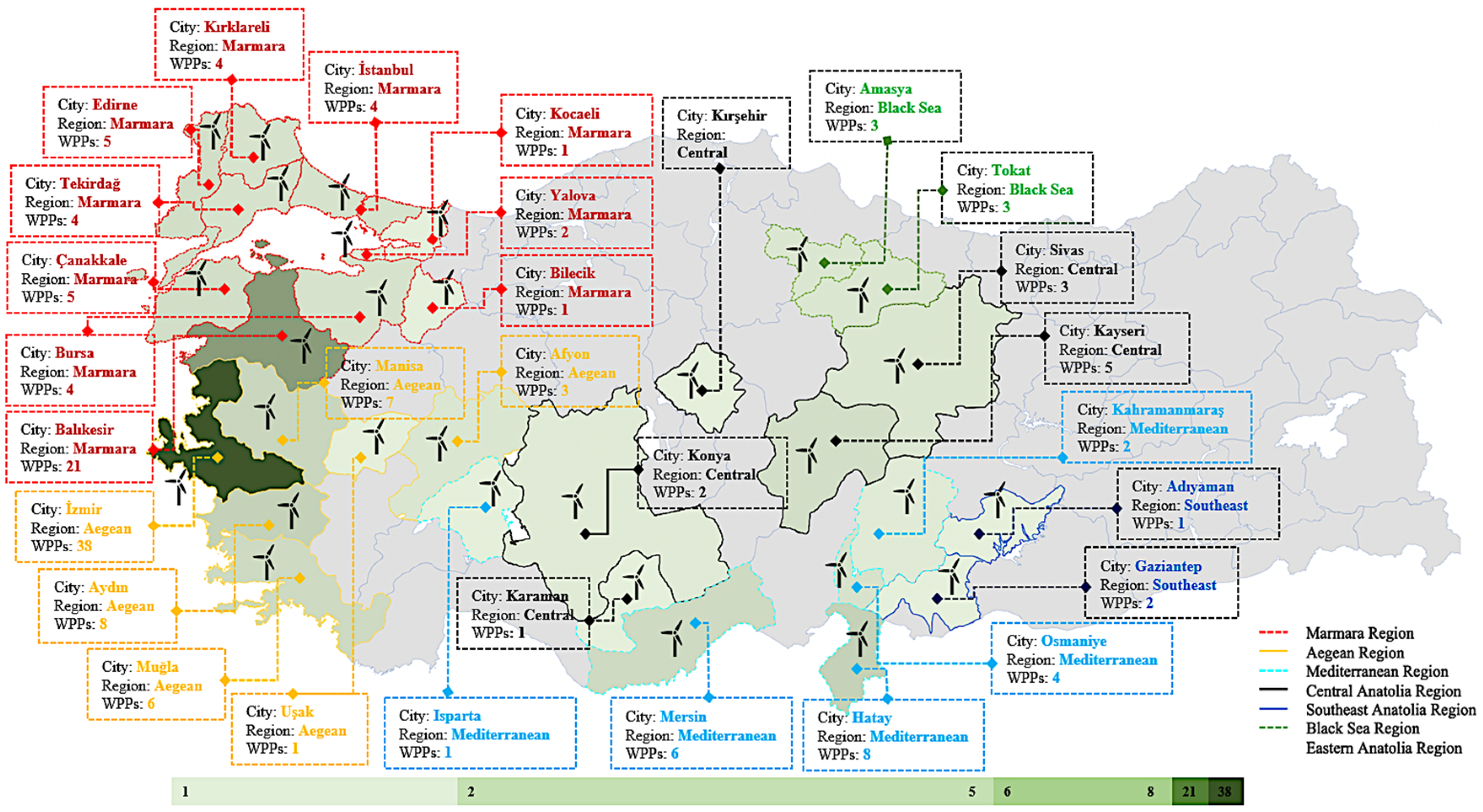
The methodology of the study was developed to optimize the wind power plants (WPPs) in order to produce maximum energy output using the historical data of operational WPPs in Turkey. There are 155 WPPs located in Turkey from which the data belonging to 2017 and 2018 were collected [21]. The wind turbines of Turkey are installed in six of the seven physiographic regions of Turkey. However, they are more concentrated in the Aegean and Marmara regions as quantitively displayed in Figure 1. The main reasons for the establishment of a large number of WPPs in these areas are the large population, heavy industry, high-altitude lands having the wind speed higher than the average of Turkey, etc. The total number of operational WPPs is 63 in Aegean Region, 51 in Marmara region, 21 in Mediterranean region, 12 in Central Anatolian region, 6 in Black Sea region, and 2 in Southeast Anatolian region. There have been no WPPs installed in Eastern Anatolian region so far. Located in the Aegean region, İzmir is the city with the highest number of wind farms with 38 WPPs. Balıkesir, in the Marmara Region, ranks the second with 21 WPPs.

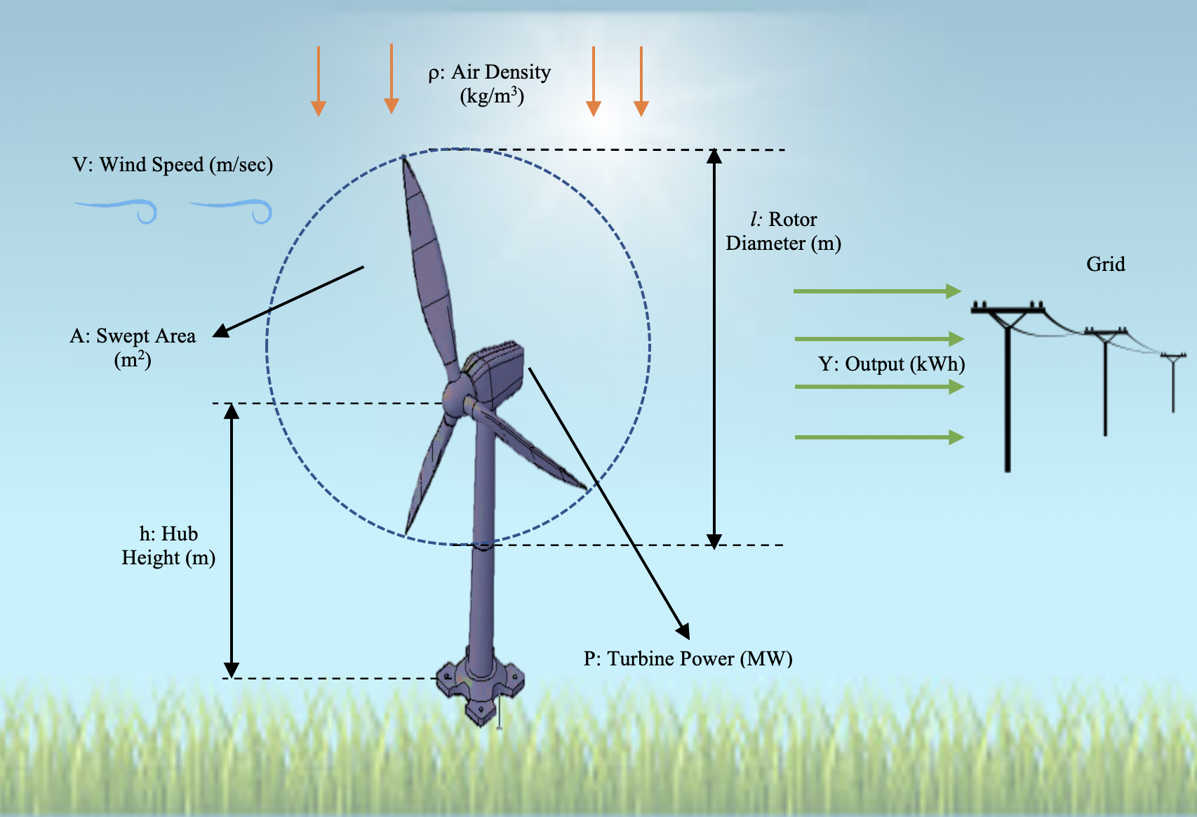
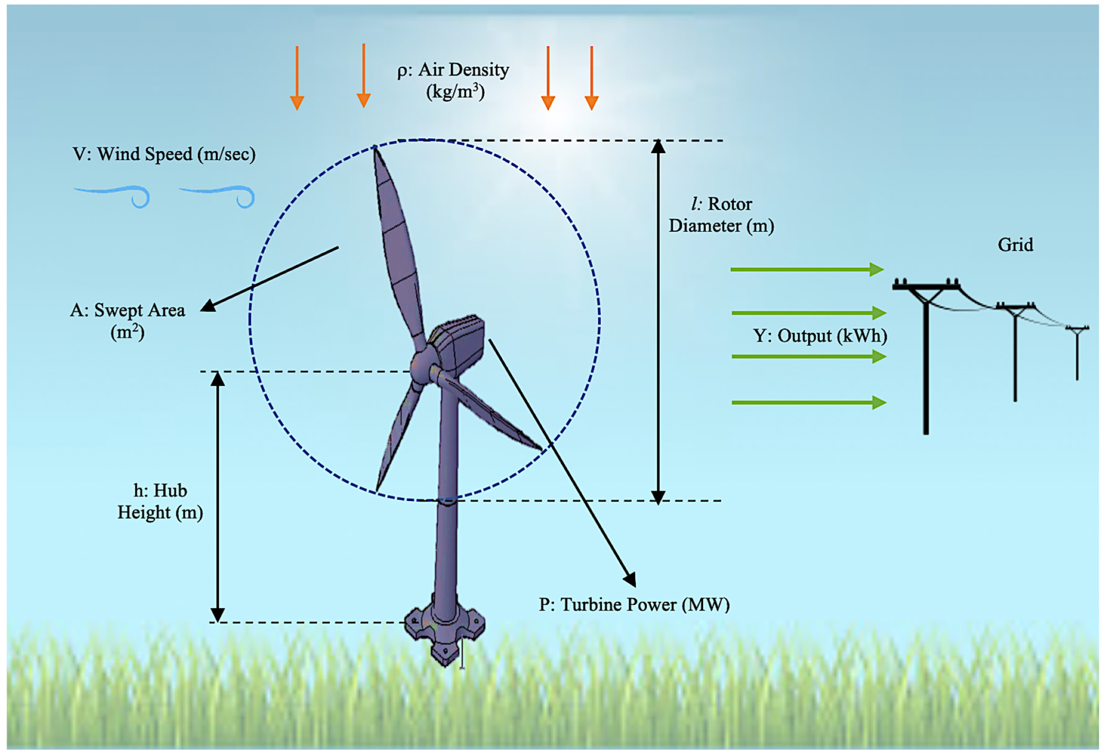
The data of 43 WPPs out of 155 were ignored due to lack or contradictory data and the fact that some wind farms have not started production yet. The contradictory data, especially for the hub height and the amount of annual produced energy, were encountered in different sources, so these WPPs were left out of the scope of this study. Additionally, some WPPs have different types of turbines (i.e., distinct turbine power, hub height and rotor diameter). Nevertheless, the data of the energy generation amount is available for the entire facility in total. Thus, these were not taken into account in order to avoid confusion in the calculations. In general, the areas with high wind speed are preferred to gain energy from wind effectively, but this is not the only factor to consider. We used hub height, rotor diameter, turbine power, and wind speed at 50 m as factors or input variables and we obtained the annual energy production amount for the years of 2017 and 2018 of the installed 112 facilities as a response or output variable (see Figure 2). Due to the fact that the number of turbines varies between the years in some WPPs, the average annual energy production per unit turbine was taken into consideration in each phase of the study.

The wind speed has an important effect on the power produced by the wind turbine. According to the study of wind speed variability and wind power potential over Turkey, Aslan et al. showed that the wind speed fitted the Weibull distribution based on hourly data of 335 stations covering 34 years [2]. Secondly, the hub height of the turbine should be taken into account concerning energy generation because of its impact on wind speed. The wind speed increases as hub height increases. The wind power-law helps to extrapolate wind speed data at different hub heights as a practical tool utilized in wind power applications. The wind profile power-law relationship is expressed as [26] (Equation (1)):

$$\frac{v}{v_0}={\left(\frac{h}{h_0}\right)}^{\alpha }$$

(1)

where $v$ is the wind speed at hub height $h$, $v_0$ is the wind speed at the initial hub height, $h_0$, and $\alpha$ is an empirically derived wind speed power-law coefficient depending on the stability of the air. The equation that shows the relationship between rotor diameter and wind speed is expressed as follows [27] (Equation (2)):

$$v=v_0\left[1-2\alpha {\left(\frac{\frac{\mathrm{l}}{2}}{\frac{\mathrm{l}}{2}+\alpha x}\right)}^2\right]$$

(2)

where $\mathrm{l}/2$ is the radius of the rotor, and $x$ is axial induction factor [28]. With the aid of the combination of the equations explained above, the extractable wind power by the turbine rotor is given by (Equation (3)):

$$P_{maxE}=\frac{1}{2}\rho A{v}^3{c}_p$$

(3)

where $A$ donates the swept area of the turbine, $c_p$ symbolizes the power coefficient. The power coefficient is defined as the percent of the extraction of the energy by a wind turbine which is 59.3 % at the most, theoretically. The value of c_p is given as [29] (Equation (4)):

$$c_p=0.593, \mathrm{referred} \mathrm{to} \mathrm{as} \mathrm{the} \mathrm{Betz} \mathrm{limit}$$

(4)

The swept area of the turbine (A) in Equation (4) can be computed with the help of the equation for the area of a circle considering the length of the turbine blades as the radius of the circle during rotation [30] (Equation (5)):

$$A=\pi l^2$$

(5)

where l represents the value of the blade length as the radius of the rotor.

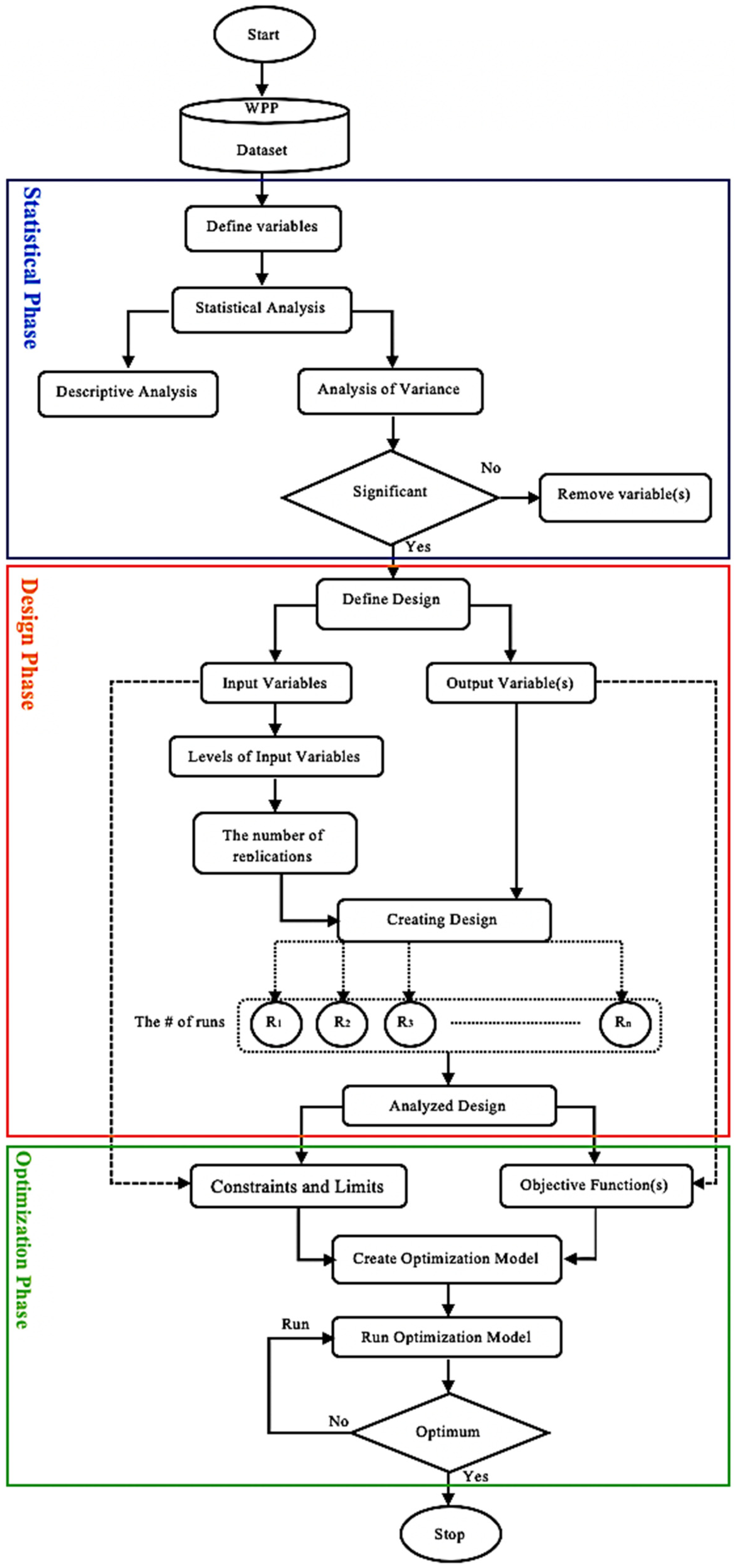
The flow chart in Figure 3 illustrates the phases of the study in detail. There are three main phases to build the methodology of the study, which are statistical analysis, Box-Behnken design of experiment (DOE) and nonlinear optimization model. Each phase constitutes the infrastructure of the next phase.

2.1. Statistical Analysis

The production of energy amount by the WPPs operated in the provinces of Turkey was organized for the analysis. Statistical analysis is the basis for constructing the next steps of the methodology of this study. The first phase before applying the DOE with the optimization method is to arrange the statistical data descriptively. Quartiles (denoted as q₁, q₂ and q₃) were used in order to separate the whole data set, belonging to 112 WPPs operating in Turkey, into three parts that help to have an idea about the distribution of the data.

Table 1. Descriptive statistics of inputs and responses.

Variables		Unit	N	Mean	SD	Min	q1	q2 (Median)	q3	Max
Factors	Turbine Power	MW	112	2.6277	0.5525	0.8000	2.1000	2.7500	3.0000	3.6000
	Hub Height	m	112	86.294	9.520	64.000	80.000	85.000	91.000	117.000
	Rotor Diameter	m	112	101.97	13.93	52.900	90.00	103.00	113.00	126.00
	Wind speed	m/s	112	6.8000	0.5075	5.4000	6.5000	6.8000	7.0000	7.7500
Response	Annual energy production in 2018	million kWh	112	6.8284	2.4234	0.1928	5.1172	6.8462	8.7195	11.9324
	Annual energy production in 2017	million kWh	112	5.8219	3.0918	0.3288	3.4548	5.7695	8.2366	12.5206

Note 1: Unit: the measurement unit; MW: megawatts; m: meters; m/s: meter per second; kWh: kilowatt-hour. Note 2: N: the number of WPPs (wind power plants) operated; Mean: the average value, Min: the minimum value, Max: the maximum value: SD (standard deviation) is a criterion to calculate the dispersion or variation quantity belonging to a data set. In statistics, data are divided into three parts to form quartiles in order to understand the distribution of the data set; q₁: 25% of the data set is less than or equal to this value; q₂ (median): 50% of the data set is less than or equal to this value; q₃: 75% of the data set is less than or equal to this value.

shows the descriptive statistics of the factors and responses.

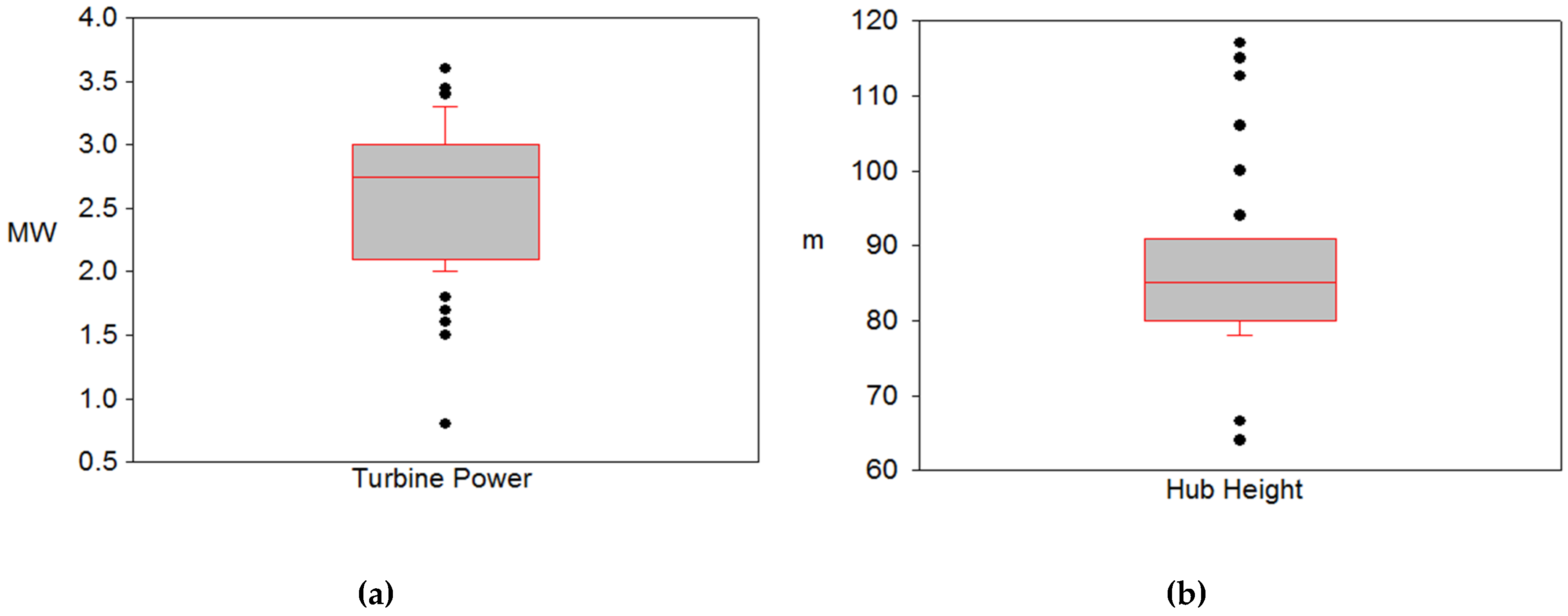
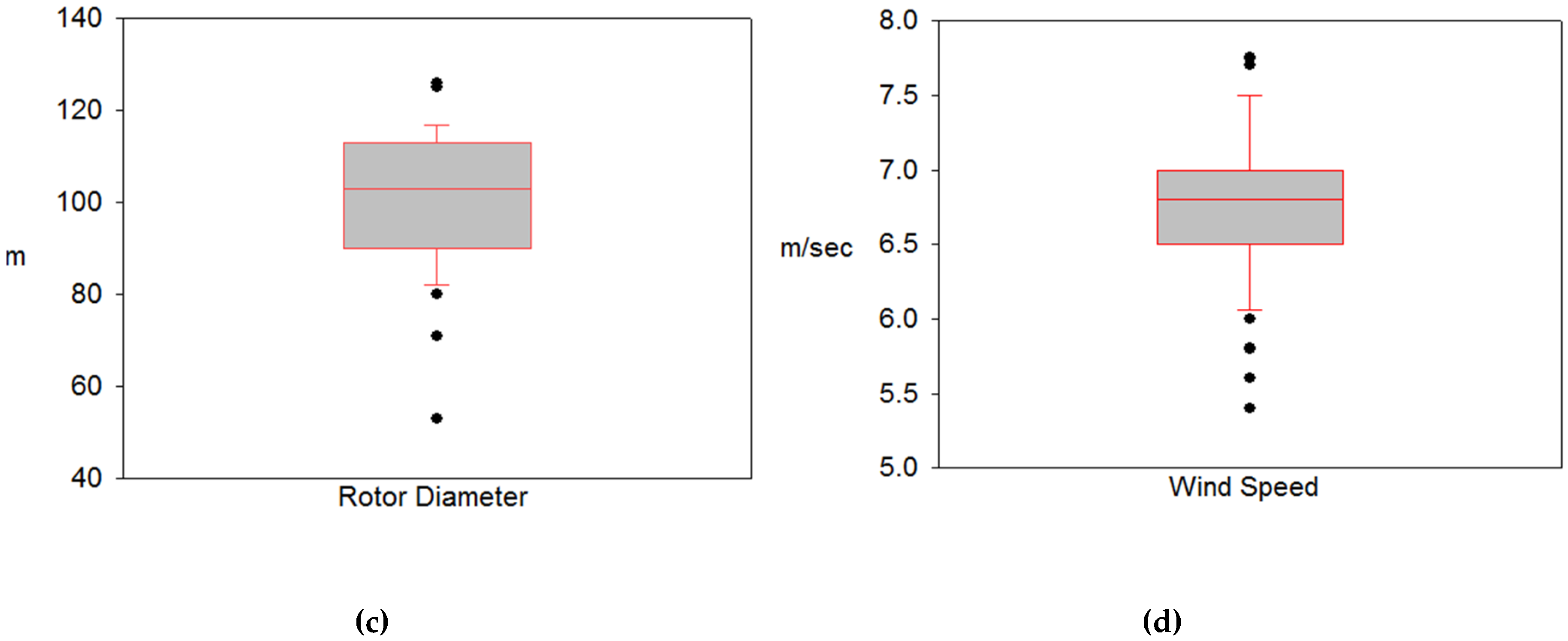
The Box plots of the four factors, namely turbine power, hub height, rotor diameter and wind speed, were generated to visually show the spread of the data set by making use of minimum value, q₁ (first quartile), q₂ (second quartile or median), q₃ (third quartile) and maximum value of each variable. As seen from Figure 4, the data of turbine power are mostly centered in the 1st quartile (2.1 MW–2.75 MW). Similarly, the data of rotor diameter and wind speed are almost concentrated in the q₁. However, hub height values are distributed more intensely in the 3rd quartile ranging from 92 m to 117 m. The intervals of quartiles for each factor are tabulated in the design part in detail.

2.2. Box-Behnken Design of Experiment

Designed experiments are useful to ascertain cause-and-effect relationships for the process of interest, which in turn help on the optimization of the response variable. DOE assists in maximizing the correctness of the result or response of a process conversely with minimizing the quantity of experiments, to escalate the system performance. DOE not only helps to specify the most important factors that influence the output but also points out the interactions among them [31]. The components of the design of experiment approach are composed of factors or variables, levels and responses [32,33]. Factors, as controllable and uncontrollable, are the input variables of the process [34]. Levels are the settings related to each factor of the system. Outputs or responses are the constituents that determine the process performance.

Models are frequently utilized in the engineering field to formulate and solve any kind of problem. The model employed for DOE to show the relationship between the response (y) (i.e., produced energy annually) and the input variables (x’s) (i.e., hub height, turbine power, rotor diameter and wind speed) is expressed as (Equation (6)):

$$y={\beta }_0+{\displaystyle \sum _{i=1}^p}{\beta }_i{x}_i+{\displaystyle \sum _{i=1}^p\sum _{j=1}^p}{\beta }_{ij}{x}_i{x}_j+{\displaystyle \sum _{i=1}^p\sum _{j=1}^p\sum _{k=1}^p}{\beta }_{ijk}{x}_i{x}_j{x}_k \left( i\ne j\ne k\right).$$

(6)

where ${\beta }_0$ is the overall mean response, ${\beta }_i$ is the main effects for each factor $\left(i=1,2,3,\dots .,p\right)$, ${\beta }_{ij}$ is the two-way interaction between $i\mathrm{th}$ and $j\mathrm{th}$ factors, ${\beta }_{ijk}$ is the three-way interaction between $i\mathrm{th}$, $j\mathrm{th}$ and $k\mathrm{th}$ factors.

Box-Behnken design (BBD), one of the subsets of DOE methodology, helps to develop higher-order models that need fewer runs as compared to other factorial designs. Thus, application of BBD not only saves time but also reduces cost with the help of decreasing the number of experiments. BBD aims to optimize the output of a system with fewest runs by combining the mathematical and statistical methods necessary for the optimization modeling and analysis of experiments where output is affected by multiple factors [33].

In this study, the BBD tool was applied to improve wind energy production process and point out the interactions among considered parameters. This design type was chosen because of the fact that it requires less design studies. More specifically, in the full-factorial experimental design with three factors having three levels of each factor, the number of designs is 162 (81 × 2) with two replicates, while the number of required designs is only 54 (27 × 2) in BBD tool. Based on BBD method, the process yield (y) is given as (Equation (7)):

$$y=f \left(x_{1 , }{x}_{2 , }{x}_{3 , }\dots , x_n\right)+ϵ$$

(7)

where $x_{i }$ denotes the numbers of factors maximizing the yield, y, of a process and 𝜖 symbolizes the noise or error observed in the response y.

The limits for the levels of variables required for the BBD design were individually determined using Box plots of the factors. The number of levels for each parameter was chosen as 3. The levels and limit values of factors are depicted in

Table 2. Coded factors levels and limits.

Factors	Notations	Level 1		Level 2		Level 3
		Coded Level −1		Coded Level 0		Coded Level 1
		Value	Limit	Value	Limit	Value	Limit
Turbine Power	A	0.8	0.8–2.1	2.2	2.11–3.0	3.6	3.1–3.6
Hub Height	B	64	64–80	90.5	81–91	117	92–117
Rotor Diameter	C	52.90	52.90–90	89.45	91–113	126	92–126
Wind Speed	D	5.40	5.4–6.5	6.575	6.6–7	7.75	7.1–7.75

.

In this research, four different factors, each having three levels, were considered with regard to their effects on wind energy production. While the number of basic designs is 27 in Box-Behnken design, the total number of data used is 54 by replicating the study twice.

Table 3. Box-Behnken design of experiment according to coded factor levels.

Proposed Types of WPP	The Features of WPPs
	Coded Levels				Actual Levels
	Factor 1 Unit 1	Factor 2 Unit 2	Factor 3 Unit 3	Factor 4 Unit 4	A (MW)	B (m)	C (m)	D (m/s)
WPP 1.0	−1.00	−1.00	0.00	0.00	0.8	64.0	89.45	6.575
WPP 2.0	1.00	−1.00	0.00	0.00	3.6	64.0	89.45	6.575
WPP 3.0	−1.00	1.00	0.00	0.00	0.8	117.0	89.45	6.575
WPP 4.0	1.00	1.00	0.00	0.00	3.6	117.0	89.45	6.575
WPP 5.0	0.00	0.00	−1.00	−1.00	2.2	90.5	52.90	5.400
WPP 6.0	0.00	0.00	1.00	−1.00	2.2	90.5	126.0	5.400
WPP 7.0	0.00	0.00	−1.00	1.00	2.2	90.5	52.90	7.750
WPP 8.0	0.00	0.00	1.00	1.00	2.2	90.5	126.0	7.750
WPP 9.0	−1.00	0.00	0.00	−1.00	0.8	90.5	89.45	5.400
WPP 10.0	1.00	0.00	0.00	−1.00	3.6	90.5	89.45	5.400
WPP 11.0	−1.00	0.00	0.00	1.00	0.8	90.5	89.45	7.750
WPP 12.0	1.00	0.00	0.00	1.00	3.6	90.5	89.45	7.750
WPP 13.0	0.00	−1.00	−1.00	0.00	2.2	64.0	52.90	6.575
WPP 14.0	0.00	1.00	−1.00	0.00	2.2	117.0	52.90	6.575
WPP 15.0	0.00	−1.00	1.00	0.00	2.2	64.0	126.0	6.575
WPP 16.0	0.00	1.00	1.00	0.00	2.2	117.0	126.0	6.575
WPP 17.0	−1.00	0.00	−1.00	0.00	0.8	90.5	52.90	6.575
WPP 18.0	1.00	0.00	−1.00	0.00	3.6	90.5	52.90	6.575
WPP 19.0	−1.00	0.00	1.00	0.00	0.8	90.5	126.0	6.575
WPP 20.0	1.00	0.00	1.00	0.00	3.6	90.5	126.0	6.575
WPP 21.0	0.00	−1.00	0.00	−1.00	2.2	64.0	89.45	5.400
WPP 22.0	0.00	1.00	0.00	−1.00	2.2	117.0	89.45	5.400
WPP 23.0	0.00	−1.00	0.00	1.00	2.2	64.0	89.45	7.750
WPP 24.0	0.00	1.00	0.00	1.00	2.2	117.0	89.45	7.750
WPP 25.0	0.00	0.00	0.00	0.00	2.2	90.5	89.45	6.575
WPP 26.0	0.00	0.00	0.00	0.00	2.2	90.5	89.45	6.575
WPP 27.0	0.00	0.00	0.00	0.00	2.2	90.5	89.45	6.575

represents all possible combinations of factors according to the Box-Behnken design of experiment both with coded levels and actual levels of each variable. Factor 1, factor 2, factor 3 and factor 4 terms are the basic names used in Box-Behnken design of experiment, and their values are denoted as −1.0, 0 and 1.0 for level 1, level 2 and level 3, respectively. The factors used for this study were replaced by actual values corresponding to these notations.

2.3. Nonlinear Optimization Models

Optimization models are developed so as to determine the optimum decision variables that meet the objective function(s) (by maximizing and/or minimizing) of any problem to be examined [35]. In many interesting maximization and minimization problems, the objective(s) or constraint(s) may not follow a linear trend, making them hard to solve. This type of optimization model is called to be nonlinear [36]. We observed that the optimization model obtained in this study fits into a nonlinear mathematical modeling type. The reason is that the factors were taken into account both singularly and interactively in the optimization model. The objective function of the nonlinear optimization model is formulated as the following [37] (Equation (8)):

$$\max or\min Z=f \left(x_{1 }, x_{2 }, x_{3 }, \dots , x_n\right).$$

(8)

The set of all points $\left(x_{1 }, x_{2 }, x_{3 }, \dots , x_n\right)$ such that $x_i$ is a real number is $R^n$. The following subsets of $R^n$ (called intervals) will be of particular interest (Equation (9)):

$$\left[l_i, u_i\right]=\mathrm{all} x \mathrm{satisfying} l_i\le x_i\le u_i$$

(9)

where $l_i, u_i$ represent lower limit and upper limit for the constraints, respectively.

The aim of this experiment is to get the maximum amount of energy produced in wind power plants. The objective of the proposed nonlinear programming model is to maximize the estimated objective function subject to the boundary constraints over the experimental region. The nonlinear model that contains all factors neglecting significance levels of the model is given as below (see Appendix A for detailed equation) (Equation (10)):

$$\begin{array}{cc}\hfill y_{kWh}={\beta }_0+{\beta }_{1}A& +{\beta }_{2}B+{\beta }_{3}C+{\beta }_{4}D+{\beta }_{11}{A}^2+{\beta }_{22}{B}^2+{\beta }_{33}{C}^2+{\beta }_{44}{D}^2+{\beta }_{12}AB\hfill \\ & +{\beta }_{13}AC+{\beta }_{14}AD+{\beta }_{23}BC+{\beta }_{24}BD+{\beta }_{34}CD.\hfill \end{array}$$

(10)

This regression equation is defined as an objective function in this study, where $y_{kWh}$ refers to the output of the WPPs (as million kilowatt-hours). Then, the full optimization model is expressed as (Equation (11)):

$$\begin{array}{c}to maximize y_{kWh}\\ \hspace{1em}\hspace{1em}=\{{\left[TP\left(A\right), h\left(B\right), l\left(C\right), v\left(D\right)\right]}_1, {\left[TP\left(A\right), h\left(B\right), l\left(C\right), v\left(D\right)\right]}_2, \dots , {\left[TP\left(A\right), h\left(B\right), l\left(C\right), v\left(D\right)\right]}_j\}\\ subject to\\ \hspace{1em}\hspace{1em}0.8\hspace{0.17em}\mathrm{MW}\le x_{Aj}\le 3.6\hspace{0.17em}\mathrm{MW}\hspace{1em}\hspace{1em}\hspace{1em}\hspace{1em}\hspace{1em}\hspace{1em}\hspace{1em}\hspace{1em}\hspace{1em}\hspace{1em}\hspace{1em}\hspace{1em}\hspace{1em}\hspace{1em}\hspace{1em}\hspace{1em}\hspace{1em}\hspace{1em} \mathrm{the} \mathrm{value} \mathrm{of} \mathrm{factor} \mathrm{A} \mathrm{for} \mathrm{the} j^{th} \\ \mathrm{WPP}\\ \hspace{1em}\hspace{1em}64\hspace{0.17em}\mathrm{m}\le x_{Bj}\le 117\hspace{0.17em}\mathrm{m}\hspace{1em}\hspace{1em}\hspace{1em}\hspace{1em}\hspace{1em}\hspace{1em}\hspace{1em}\hspace{1em}\hspace{1em}\hspace{1em}\hspace{1em}\hspace{1em}\hspace{1em}\hspace{1em}\hspace{1em}\hspace{1em}\hspace{1em}\hspace{1em}\hspace{1em}\hspace{1em} \mathrm{the} \mathrm{value} \mathrm{of} \mathrm{factor} \mathrm{B} \mathrm{for} \mathrm{the} j^{th} \\ \mathrm{WPP}\\ \hspace{1em}\hspace{1em}52.9\hspace{0.17em}\mathrm{m}\le x_{Cj}\le 126\hspace{0.17em}\mathrm{m}\hspace{1em}\hspace{1em}\hspace{1em}\hspace{1em}\hspace{1em}\hspace{1em}\hspace{1em}\hspace{1em}\hspace{1em}\hspace{1em}\hspace{1em}\hspace{1em}\hspace{1em}\hspace{1em}\hspace{1em}\hspace{1em}\hspace{1em}\hspace{1em}\hspace{1em} \mathrm{the} \mathrm{value} \mathrm{of} \mathrm{factor} \mathrm{C} \mathrm{for} \mathrm{the} j^{th} \\ \mathrm{WPP}\\ \hspace{1em}\hspace{1em}5.4\hspace{0.17em}\mathrm{m}/\mathrm{s}\le x_{Dj}\le 7.75\hspace{0.17em}\mathrm{m}/\mathrm{s}\hspace{1em}\hspace{1em}\hspace{1em}\hspace{1em}\hspace{1em}\hspace{1em}\hspace{1em}\hspace{1em}\hspace{1em}\hspace{1em}\hspace{1em}\hspace{1em}\hspace{1em}\hspace{1em}\hspace{1em}\hspace{1em} \mathrm{the} \mathrm{value} \mathrm{of} \mathrm{factor} \mathrm{D} \mathrm{for} \mathrm{the} j^{th} \mathrm{WPP}\\ x_{ij}, nonnegative\\ x_{ij}\in R^n\end{array}$$

(11)

where $i=\left\{A,B,C,D\right\}$, and $j=\left\{the assigned of WPP\right\}$. According to the BBD of experiment, a total of $27\times 2$ different WPPs have been designed with different factor values for optimum WPP design, generating maximum annual energy. The limits of the constraints have been determined by BBD.

Furthermore, the development of additional optimization models for the mean and standard deviation of the response variable are required simultaneously to improve the optimization process. The idea behind this concept is to maximize the mean value and minimize the standard deviation of outputs symbolized by $y$ [38]. The use of BBD method necessitates to minimize the standard deviation to reach the target value for industrial problems. Thus, we have extended the developed optimization models with this approach since wind power generation is a real industrial issue worldwide. The polynomial models for the mean ($y_{\mu }$) and standard deviation ($y_{\sigma }$) of the response were formed by Vining and Myers as following [39] (Equations (12) and (13)):

$$y_{\mu }={\beta }_0+{\displaystyle \sum _{i=1}^k}{\beta }_i{x}_i+{\displaystyle \sum _{i=1}^k}{\beta }_{ii}{x}_i^2+{\displaystyle \sum _{i=1}^k\sum _{j=1}^k}{\beta }_{ij}{x}_i{x}_j+{\epsilon }_{\mu } i<j,$$

(12)

$$y_{\sigma }={\gamma }_0+{\displaystyle \sum _{i=1}^k}{\gamma }_i{x}_i+{\displaystyle \sum _{i=1}^k}{\gamma }_{ii}{x}_i^2+{\displaystyle \sum _{i=1}^k\sum _{j=1}^k}{\gamma }_{ij}{x}_i{x}_j+{\epsilon }_{\sigma } i<j$$

(13)

where ${\beta }_0, {\beta }_1, {\beta }_2, \dots , {\beta }_k$_, and ${\gamma }_0, {\gamma }_1, {\gamma }_2, \dots , {\gamma }_k$ are regression coefficients,$x_{i }$ is the number of the factors, and ${\epsilon }_{\mu }$ and ${\epsilon }_{\sigma }$ are the random errors of the mean and standard deviation of the response variable, respectively. Determining the values which minimize performance deviation from the target value is preferable. The additional optimization models were introduced as below (see Equations (14) and (15)):

$$\begin{gathered} Minimize {\widehat{y}}_{\sigma }=f {\left(x_{1 , }{x}_{2 , }{x}_{3 , }\dots , x_n\right)}_{\sigma } \\ Subject to f {\left(x_{1 , }{x}_{2 , }{x}_{3 , }\dots , x_n\right)}_{\mu }={\tau }_{\mu } \\ {\tau }_{\sigma } , x_i, nonnegative \\ {x}_i\in R^n \end{gathered}$$

(14)

$$\begin{gathered} Maximize {\widehat{y}}_{\mu }=f {\left(x_{1 , }{x}_{2 , }{x}_{3 , }\dots , x_n\right)}_{\mu } \\ Subject to f {\left(x_{1 , }{x}_{2 , }{x}_{3 , }\dots , x_n\right)}_{\sigma }={\tau }_{\sigma } \\ {\tau }_{\sigma }, x_i, nonnegative \\ {x}_i\in R^n \end{gathered}$$

(15)

where ${\tau }_{\mu }$ and ${\tau }_{\sigma }$ are the target values of the mean and standard deviation of outputs. ${\widehat{y}}_{\mu }$ and ${\widehat{y}}_{\sigma }$ represent the functions of regressions. Target values represent the points corresponding to the constraints of the optimization models developed for the study.

3. Results and Discussion

This study involves the application of Box-Behnken design that is part of the design of experiment with a total of 54 runs (27 base runs with two replications), while considering four variables, each with three levels, for the wind power plants to provide maximum energy produced. The factors, which are turbine power, hub height, rotor diameter and wind speed denoted as A, B, C and D, respectively, were analyzed statistically. Furthermore, R², the value of the coefficient of multiple terms for the regression showing the statistical measure of how close the data are to the fitted regression line, was calculated as 0.9179 (R² adj is 0.8885). With regard to the statistical analysis, the individual and interactive effects of factors were determined by calculating F-value, t-Ratio and p-value. According to

Table 4. Analysis of variance for factors of wind power.

Source	Model Types	F-Value (1.5017)	t-Ratio (2.02)	Prob>|t| Prob>|F|	Status
Model		31.160	29.00	<0.001	Significant
A	Linear	237.87	15.42	<0.001	Significant
B		4.6400	−2.15	0.037	Significant
C		62.040	7.88	<0.001	Significant
D		12.040	−3.47	0.001	Significant
AA	Square	37.440	−6.12	< 0.002	Significant
BB		3.6600	−1.191	0.063 *	Significant *
CC		4.9100	−2.22	<0.033	Significant
DD		34.880	−5.91	<0.001	Significant
AB	2-way Interaction	1.5900	1.26	0.215	Insignificant
AC		2.7800	1.67	0.103	Insignificant
AD		24.010	3.07	<0.001	Significant
BC		9.4400	4.90	<0.004	Significant
BD		5.8800	−2.42	<0.020	Significant
CD		19.790	−4.45	<0.001	Significant

Note: p-value < 0.05, if the individual and interactive effects of the factors that could influence the response and are statistically significant; * at the margin of statistical provisionally significance (p-value < 0.1); Prob>|t| the p-value associated with a two-tailed test.

, it is seen that the overall model, the factors (linear) and the interactions with themselves (square) are important for the production of wind energy (p-value ≤ 0.05). However, when the 2-way interactions are considered, it is understood that the interactions of factor A (turbine power) with factors B (hub height) and C (rotor diameter) are insignificant in terms of the amount of energy generated (p-value ≥ 0.05).

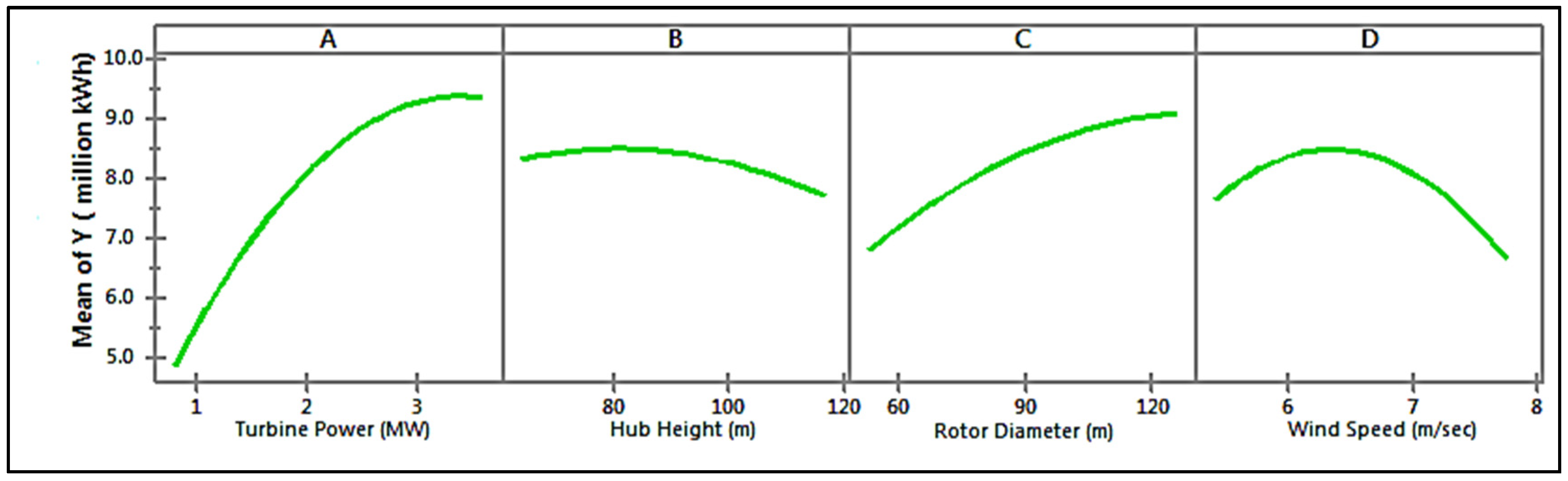
The main effects plot was made to show how the mean of response changed concerning the levels of each factor. The impact of factors (A, B, C and D) on the response variable (Y) is separately demonstrated in Figure 5. It has been observed that the response variable increases up to a certain point with the increase of factors A and C. Increasing the level of factor B had a very low positive effect on the outcome. As seen from the figure, the increase in the level of wind speed (factor D) escalated the result variable up to a certain point and then started decreasing. The similarity between these separate curves that show the effect of each factor on energy production in WPPs was that they all followed a nonlinear trend.

After investigating individual and interactive impacts of each factor on response with their significance degrees by statistical analysis, a nonlinear optimization model (defined in the previous section) was established to find out the optimum values of input and output variables. The objective function of the initial model is to maximize the annual energy output per unit turbine, which is defined as Target₀.

The desirability values check the validity of the results obtained in the optimization models. Desirability value, ranging from 0.0 to 1.0, evaluates how well the combination of variables meets the objectives defined for the answers. The closer this value to 1.0, the better the desired objective function value is. The optimum results with high desirability value (0.9587) for factors A, B, C, D were calculated as 3.0670 MW, 108.8424 m, 106.7597 m, 6.1684 m/s, respectively, to produce the maximum amount of annual energy which is estimated to be 9.952 million kWh per unit turbine. The best ten feasible solutions, according to their desirability values, are represented in descending order in

Table 5. Best ten solutions for Target₀ ($y_{kWh}$) based on desirability value.

Feasible Solutions	A (MW)	B (m)	C (m)	D (m/s)	Target0 (Million kWh)	Desirability Values
1.0	3.06700	108.842	106.759	6.16840	9.9552	0.95870
2.0	3.60000	103.627	125.319	7.28635	9.8343	0.94530
3.0	3.25161	77.4070	116.904	5.92158	9.5293	0.91058
4.0	1.68100	116.695	126.000	5.40000	9.2783	0.88203
5.0	3.60000	68.0000	118.867	7.33282	9.1664	0.86929
6.0	3.60000	64.0000	56.0950	7.73137	8.8958	0.83849
7.0	2.13088	74.5810	126.000	5.49682	8.6917	0.81527
8.0	2.20000	90.5000	89.4500	6.57500	8.4555	0.78839
9.0	3.16695	112.383	81.2810	6.18659	8.3459	0.77593
10.0	2.27123	64.3830	79.5340	6.47867	8.2612	0.76629

. This table includes the top ten feasible results for turbine power (A), hub height (B), rotor diameter (C) and wind speed (D) and gives the annual average amount of energy per unit turbine with these configurations.

The optimization process was improved with additional optimization models developed for the mean and standard deviation of the response variable. The optimization results when the mean of output is maximized while keeping the standard deviation constant is stated as Target₁ (max $y_{kWh}$ of output subject to constant ${\widehat{y}}_{\sigma }$). The optimization results of the mean of output for the factors A, B, C, D and the response were calculated as 2.9395 MW, 101.1193 m, 94.7760 m, 6.4038 m/s, and 9.390 million kWh per unit turbine, respectively, with the desirability value of 0.9246.

The second optimization model presents the situation in which standard deviation is minimized while holding mean of response at a constant level that is expressed as Target₂ (min ${\widehat{y}}_{\sigma }$ subject to constant $y_{kWh}$). The optimum results, with high desirability value of 0.9144, for the factors A, B, C, D and the response were computed as 1.7665 MW, 106.2929 m, 95.4418 m, 6.8004 m/s, and 7.143 million kWh per unit turbine, respectively. The minimized standard deviation value of response was computed as 0.24680 million kWh.

The multi-objective optimization (max $y_{kWh}$ and min ${\widehat{y}}_{\sigma }$) of output results, in which mean of response is maximized (Target₁) while standard deviation is minimized (Target₂), simultaneously, are shown in

Table 6. The results of all optimization models.

	Input Factors				Target0 ${\mathit{y}}_{\mathit{k}\mathit{W}\mathit{h}}$	Target1 ${\widehat{\mathit{y}}}_{\mathit{\mu }}$	Target2 ${\widehat{\mathit{y}}}_{\mathit{\sigma }}$
Optimization Models	A (MW)	B (m)	C (m)	D (m/se)	Maximize (Million kWh)	Maximize (Million kWh)	Minimize (Million kWh)	Composite Desirability (0.0 < CD> 1.0)
Target0	3.0670	108.8424	106.7597	6.1684	9.952	Constant	Constant	0.95872
Target1	2.9395	101.1193	94.7760	6.4038	-	9.390	Constant	0.92460
Target2	1.7665	106.2929	95.4418	6.8004	-	Constant	0.24680	0.91440
Multi-Objective	2.7100	94.5152	112.0857	6.6581	-	9.684	0.28630	0.91560
Average	2.62075	102.6925	102.2658	6.50767	9.952	9.537	0.26655	0.92833

. It can be evaluated as the combinational representation of the results of the optimization models concerning both mean and standard deviation of output. The optimum results, having desirability value of 0.9156, for the factors A, B, C, D and the output were calculated as 2.7100 MW, 94.5152 m, 112.0857 m, 6.6581 m/s, and 9.684 million kWh per unit turbine, respectively. The minimized standard deviation value of output was 0.28630 million kWh.

The results of all optimization models with their desirability values were displayed together in Table 6. The averages of all optimum results were computed for the factors A, B, C, D as 2.62075 MW, 102.6925 m, 102.2658 m, and 6.50767 m/s, respectively, with a high average desirability value of 0.92833, to get maximum energy production which was 9.952 million kWh in Target₀, 9.537 million kWh in Target₁ per unit turbine. The average of the standard deviation of the response variable was calculated as 0.26655 million kWh in Target₂.

In terms of the validation of the method used, we have optimized each decision variable separately by fixing the other three decision variables according to the mean value of parameters which was determined as the reference case.

Table 7. The comparison of the decision variables’ results.

	A (MW)	B (m)	C (m)	D (m/s)	Optimum 1	Optimum 2	Differences (%)
A (MW)	0.8–3.6	Fixed (86.294)	Fixed (101.97)	Fixed (6.80)	2.710	2.723	0.4790%
B (m)	Fixed (2.627)	64–117	Fixed (101.97)	Fixed (6.80)	94.5152	95.05	0.5658%
C (m)	Fixed (2.627)	Fixed (86.294)	52.9–126	Fixed (6.80)	112.0857	112.709	0.5560%
D (m/s)	Fixed (2.627)	Fixed (86.294)	Fixed (101.97)	5.4–7.75	6.6581	6.6106	0.7100%

Optimum ¹: The optimum results of the decision variables based on multi-objective functions’ optimization models. Optimum ²: The optimum results of the decision variables based on a reference case in which one constraint is optimized at a time and three other constrains are fixed.

shows the comparative results of decision variables of multi-objective functions’ optimization models and the findings after validation process. The percent difference between the optimum values of each variable is way below 1%, demonstrating that the applied method and the results are more than 99% confident.

The European Wind Energy Union classifies wind speeds as nearly good for 6.5 m/s, good for 7.5 m/s and very good for 8.5 m/s which is suitable for energy generation from wind [40]. All of the optimization models developed propose that even in areas in nearly good wind speed group, the higher amount of wind energy can be produced with optimizing other variables. In terms of comparison, Lee et al. investigated the optimization of hub height to get maximum annual net profit. They limited the hub height value between 30 m and 300 m in the optimization model developed for WPPs. The optimum hub height value they find is 125.8 m with $V=7$ m/s and $\alpha =0.25$ for case 1 and 219.2 m with $V=5$ m/s and $\alpha =0.3$ for case 2 [41]. One of the most important factors affecting the initial capital cost in WPPs is the hub height. Therefore, we can assume that the hub height value we calculated in this study, which is 105 m, is more reasonable in terms of cost. Lee et al. calculated the optimum hub height value as 75 m, which is calculated by considering the cost of establishment. However, the amount of energy produced according to the calculated hub height is low in their study [41]. Cheng et al. studied the optimization of rotors for higher power capture from the wind. They tried to optimize Darrieus-type vertical axis wind turbine rotor having a constant turbine power of 5 MW. The optimum value was computed as 120.96 m for rotor diameter and 143 m for hub height. Moreover, the reference height for wind speed was considered as 79.78 m [42].

In short, it was observed that the desirability values, which indicated how much the combination of the variables have achieved the target defined for the response variable(s), for all of the developed optimization models were close to 1 and very similar to each other. This closeness supports the feasibility of our study, which might assist not only operators but also researchers, entrepreneurs and governments for the future.

4. Conclusions

This study focuses on gaining maximum benefit from wind energy that has the potential to meet increasing energy demands in a cost-effective and environmentally friendly way without depending on fossil fuel sources. In this respect, the data from operating wind power plants in Turkey were collected to apply the design of experiment and optimization techniques together in the wind energy field for the first time in such a comprehensive manner. Turbine power, hub height, rotor diameter and wind speed (at 50 m) were selected as decision variables whose limits required for the design were determined using Box plots. Both the individual and interactive effects of controllable and uncontrollable factors on wind power generation were investigated with the help of Box-Behnken design. The results showed that all the input factors were significant for wind energy production based on p-value, which is the sign of the importance of the results. The 2-way interactions of the design parameters, that is, the interaction of factors with each other, were found to be significant, too, except for the interactions of turbine power with hub height and rotor diameter.

After analyzing individual and interactive impacts of each factor on the response with significance degrees, a nonlinear optimization model was established in order to find out the optimum values of input and output variables. The optimum results with high desirability value (0.9587) for the factors A, B, C, D were calculated as 3.0670 MW, 108.8424 m, 106.7597 m, 6.1684 m/s, respectively, to produce the maximum amount of energy which was 9.952 million kWh per unit turbine, annually. The optimization process was improved with additional optimization models developed for the mean and standard deviation of the response variable in the way of maximizing mean of output, minimizing standard deviation of response and combining them both. It was observed that the desirability values for all of the developed optimization models were close to 1 and very similar to each other. The similarity between these results advocates the feasibility of our study to gain the maximum amount of energy from wind power plants. The results may serve as guidelines to contribute to satisfying the escalating energy needs of the future by more sustainable and clean ways.