Activity-Based Demand Modeling for a Future Urban District

Abstract

Identifying the spatio-temporal patterns of people activities in urban areas is key to effective urban planning; it can be used in real-estate projects to predict their future impacts on behavior in surrounding accessible areas. LaVallée is a large construction project recently started in Paris’s suburb; it is a new district due in 2024. The paper is in the field of urban planning, aiming at developing a method making it possible to model the potential visits of the various equipment and public spaces of the district, by mobilizing data from census at the departmental level, and the layout of shops and activities as defined by the real-estate project. This model takes into account the flow of external visitors, estimated realistically based on the pre-project movements in the areas of influence of LaVallée. In this paper, we propose an activity-based model methodology to determine trips and their purpose at a mesoscopic scale including the city and surrounding areas, in the current baseline scenario. This travel demand is required to estimate potential external visitors of the future district. A first demonstration shows that the model correctly represents the current demands and allows the forecast of future demand in the area.

1. Introduction

1.1. Activity-Based Models

Large-scale and complex systems, in different socio-demographic contexts and various land-use configurations, can be modeled by simulating the behavior and interactions of millions of self-interested “agents”. The multi-agent paradigm provides a high level of details and allows representation of non-linear phenomena and patterns that would be difficult to tackle with analytical approaches [1]. Among multi-agent models, there is a class called activity-based models, which addresses specifically the need for realistic representation of travel demand and the human behavior in a mobility context. The activity-based modeling (ABM) framework was originally developed in response to demands for more realistic travel demand models which can analyze a wider range of transportation policies. These models generally are better able to evaluate travel demand and transportation supply management strategies, such as road pricing intelligent transportation systems, and behavior modification programs (flexible scheduling, ride-sharing), better than the previous generation of aggregate flow models which generally focus on evaluating network capacity improvement.

Recently, these models have become more widely used in practice. Activity-based models share some similarities to traditional 4-step models [2]: activities are generated, destinations for the activities are identified, travel modes are determined and, finally, the specific network facilities or routes used for each trip are predicted. However, activity-based models incorporate some significant advancements over 4-step trip-based models, such as the explicit representation of realistic constraints of time and space as well as the linkages among activities and travel both for an individual person as well as across multiple persons in a household. These linkages enable them to represent the effect of travel conditions on activity and travel choices more realistically. Activity-based models also can incorporate the influence of very detailed person-level and household-level attributes, and the ability to produce detailed information across a broader set of performance metrics. These capabilities are possible because activity-based models work at a disaggregate person-level rather than a more aggregate zone-level like most trip-based models.

In activity-based models, unlike traditional analytical trip-based models, the travel demand stems from the traveler’s needs to pursue some activities distributed in space and time. As a consequence, the understanding of the travel decisions becomes secondary compared to the fundamental understanding of the agent’s activities [3]. Based on this methodological choice, activity-based models have been proposed, such as TRANSIMS (TRansportation ANalysis SIMulation System) [4] and ALBATROSS (A Learning-Based, Transportation-Oriented Simulation System) [5]. TRANSIMS is an activity-based and an integrated system of travel forecasting and microscopic simulation models developed originally for regional transportation planning, but which was used in many other contexts since then. ALBATROSS is an activity-based model that forecasts the conducted activities, together with their location, timing and duration. It also defines the used transport modes, and the implied route decisions.

1.2. Problem Statement and Scope of the Paper

In this paper, we provide an ABM methodology to determine the trips and their purpose at a mesoscopic scale including the city and surrounding areas. The methodology is applied to LaVallée, a large construction project recently started in Paris’s suburb, due in 2024. We focus on the generation of a synthetic population that represents the current socio-demographic situation of the area, representing people who are prone to be the future users of the district.

ABM for transportation modeling requires mainly the supply infrastructure (road network), and the travel demand in the form of a set of activity plans for each agent (traveler). An activity plan is a chain of activities that will be realized during a day such as Home-Work-Home for employed individual, or Home-Education-Leisure-Home for a student. It includes the transport mode of each leg. The full set of agents is called the population.

In most of ABM literature the population is described by the set of agents and their socio-economical characteristics and aggregated information, but the process to build their activity plans is seldomly described. Except when specific disaggregated data on mobility pattern are available such as transport mode at the spatial zoning level (TAZ = Traffic Analysis Zone) [6], or tailored census in the area of interest by experts consultant which are not reproducible. For instance, the study of [7] design a travel diary survey that was executed with the Vilnius Municipality, to devise a sustainable mobility plan. They had access to a fine-grained information on important mobility parameters of activity sequences over a sample of urban population during the weekday.

We are interested in the suburb of Paris, whose population was recently modeled in [6]. In this paper the authors had access to the regional household travel survey, which is not available publicly. This survey called EGT—Global Transport Census, a Household Travel Survey specific to the Greater Paris—gathered accurate individual information about mobility patterns of a representative set of people of Great Paris area (Île-de-France). Individual travel plans are grouped into a set of a ten possible activity plans. However, the individual information of the census is not publicly available. Only aggregated information is granted public access about trip purposes and their mode, average number of trips. These data are presented for the height departments of the Greater Paris metropolis. This information is coarse if one consider a smaller region of interest, since a department can contain about a hundred Traffic Analysis Zone.

Let us consider department 92 called Hauts-de-Seine illustrated in yellow in Figure 1. From the EGT survey one can learn that for Home-Work trips, 37% of people use their car while 43% use public transportation. However, this information is not available at a smaller scale such as the grey sub-region which is defined as the catchment area of a district of interest in this study.

Specifically, we are focusing on the mobility patterns of a population over this 7 km × 8 km area surrounding an urban district of interest. This catchment area was determined as the region of attraction of the district mostly because it can be reached in less than 15 min using a private vehicle, public transportation, walking or cycling. In this catchment area, illustrated in Figure 1 (right), it is not possible to access accurate and direct fine-grained information on activity plans of people, unless we have access to unpublished data or produce our own public census.

Still some other public sources can be found at the smaller resolution of TAZ or finer from which activities can be derived: namely professional mobility census, population census and facilities location. Especially a population with a rather large variety of activity chains is required: the selected ones are illustrated in Section 6.2.

Therefore, we proposed a method to design such activity plans over the catchment area using only publicly available data. Moreover, we only used three data sources that can typically be found in other countries, while most of the other ABM population synthesis method uses much more data sources ([6] uses eight).

Even if the output model is coarse we have found the method to reflect the mobility trends experienced in the department, and it could be useful to practitioners interested in approximate flows and their mode share.

Finally, it will provide much needed insights on population synthesis methods that are often undisclosed, which is unfortunate if one need to know the amount of manual work required by this step of an ABM travel model.

The remainder of this paper is structured as follows: Section 2 gives an overview of the main approach for synthetic population generation—Synthetic Reconstruction and Combinatorial Optimization—and the data it requires. In Section 3 the context of predicting exogenous usage demand of a future district is presented, with the need for a travel demand in the district’s catchment area. Section 4 the proposed method is exposed with the technical development it requires. Section 6 exposes the travel demand model validation and the experimental results in the form of aggregated statistics, and videos of the model with spatial location of activities and individual traveler’s journeys. Section 7 concludes the article and gives perspectives of this work.

2. Literature Review

A synthetic population (SP) is an approximation of a real population (of a specific area), it exists only artificially [8]. Synthetic population generating is the first step to build an activity-based model: it is its main input.

To create a synthetic population, socio-demographic data are required, and a specific process is necessary to generate it, matching the persons and household distributions. Several approaches have been developed to generate a population, and a choice between them must be done to select those which fits the characteristics of available data. The quality of the generated population depends essentially on the quality and details’ level of the (sample) data [9]. Synthetic populations can be used as input in several models such as activity-based models (demand models) [7,10] and disease transmission models [11].

To generate a synthetic population, data are required at two levels: personal and household, these data are extracted from different sources (mainly from the census data).

Census data are the main data source. A census can be detailed on two levels: aggregate level and disaggregate level. Aggregate data are generally drawn from aggregate census dh as: Summary Files(SFs) in the United States [12], or the French Household Data in France [13] (cf.

Table 1. Example of French Household File.

CODGEO	TYPMR	NPERR	NB
Zip Code	Household Type	Household Size	Number of Households
92019	31	4	440
75015	42	5	62
77420	41	3	75

). These data are available as multi-dimensional joint distributions tables, they focus on a set of demographic and socio-economic attributes (called control variables), e.g., for individuals (age by sex by employment status), for households (housing tenure by household size by type) [14,15].

Disaggregate data represents a sample of households (or persons) with several information about their characteristics. For instance: Public-Use Microdata Samples (PUMS) [16] and French Mobility Data (home-work trips) [13] (cf.

Table 2. Example of French mobility (census) data.

Person-Id	AGEREVQ	EMPL	SEX
	Age by Range of Five Years	Employment Status
p1	020	1	2
p2	065	2	1
p3	025	1	2

). It offers details about all the control variables, but only for a sample of households (individuals) [15].

Several methods were proposed to generate a synthetic population, they require at least a representative population sample data. Access to these data presents privacy and confidentiality issues. These methods belong to two groups: Synthetic Reconstruction (SR) and Combinatorial Optimization (CO). SR approach is an earlier method for generating a synthetic population, it uses a deterministic process to reconstruct the population, by reproducing all known constraints (from census tables). The process is sequential, typically composed of two steps: the fitting step and the generating step. In the fitting step, the reference sample (selected household and individual attributes) is fitted to a set of subtotals (aggregate constraints) provided by the actual population data: it generates a fitted joint distribution [8,17]. The generating step uses the joint distribution (of the fitting step) to generate (or to expand the initial population to) a full population [18]. Person and household levels are matched through the common variables to fill the households. Several selection methods are proposed in the literature, such as: Monte-Carlo Sampling [19] and Combinatorial Optimization [20].

Two main synthetic reconstruction methods are developed: iterative proportional fitting and iterative proportional updating [21].

CO is an iterative and stochastic process proposed by [20], examined and improved by [22]; it is used to rebuild the original SP of a specific area from the pool. It is an alternative method to the SR approaches; it is a re-weighting method: It consists of re-weighting a sample to satisfy the constraints (fitting), then generating population based on these weights of an existing pool. It selects a combination of elements (individuals or households) that best fit with the specific area constraints. It finally evaluates every combination of elements from the pool, and find the set that best fit is practically unfeasible due the high computation.

The original CO approach uses the hill climbing technique [23], it starts by selecting randomly an initial set of elements from the pool; then, it applies a replacement procedure: replace an existing element with another element (from same type) from the pool; if the replacement improves the fit, the swap is applied, otherwise the swap is not made. This process is repeated until the convergence (maximum iterations, fit quality). Given the large search space, the final combination reaches the best achievable, rather than the optimal combination.

CO process maybe have only one best solution, practically, it is possible to find a good solution (relative to the constraints and acceptable levels), by using different initial combinations (it will generate swaps sequence), which lead to get different solutions. The main fit-measure is Z-score [22].

3. Case Study

3.1. LaVallée District: A Real-Estate Development

LaVallée is a large construction project recently started in Paris’s suburb. Its spatial extent is about 500 m × 400 m, part of larger city called Châtenay-Malabry. The whole district is to be delivered in 2024. As of beginning of 2020, the first roads are being built and the first inhabitants are expected by 2021. Figure 2 illustrates the present situation, and its virtual future look.

It will house 6000 residents (20% of the city population), a large set of services ranging from a shopping street, a mall, schools and office spaces for 2000 employees; and the district is designed to be opened to the rest of the city.

Buildings’ 3D visualizations give a precise architectural viewpoint of the project after completion, but as a ghost town: one need to populate it with life: people, bikes, cars, activities, etc. This is usually done by 3D simulations for commercial purposes that can be realistic in appearance but have no relation to actual people trips and future usage of urban spaces.

I-Site FUTURE and Eiffage are cofunding a project on sustainable development of cities called E3S (EcoQuartier Smart, Sustainable and Secure). University Gustave Eiffel is contributing to E3S by developing a living-lab of micromobility, and numerical methods to predict potential visits and places of interest based on mobility scenarios in the future real estate.

Based on the collection of traces left by digital ecosystems, our overall objective is to develop a method making it possible to model the potential visits of the various equipment and public spaces of the project by mobilizing data from census at the departmental level, but also from mobile applications inside LaVallée.

3.2. Travel Demand in the District’s Catchment Area: Overview

They are many ways to characterize an urban area, for example [24] estimates spatial change in urban heat island over a district using satellite imagery. Ref [25] introduces a framework to evaluate urban design in future climatic conditions based on microclimatic modeling. In [26] the impact of densification and greening strategy on the inner city of Rotterdam (business/shopping district) are studied using GIS mapping, sustainability indicators, and urban models. Our work aims at predicting the future hotspots (most visited places) of a district using travel model and land-use information.

The present paper describes a stage of a larger project willing to determine a scale indicating the quality and vitality of public spaces (the hotspots of LaVallée), based on mobility data and the layout of shops and activities. This model takes into account the flow of external visitors, estimated realistically based on the pre-project movements in the areas of influence of LaVallée.

We define the catchment area of LaVallée district as the area that can be reached by future potential visitor. Potential visits correspond to a need for a specific purpose (shopping, leisure, school) that are currently done outside of the district, but would be more convenient if realized in LaVallée, when the real estate is developed (four years from now).

Figure 3 indicates the location of the district of interest, and the catchment area where LaVallée would attract a population that will use its services. This area is defined as rather large, including not only the whole city but also surrounding cities, because it will be accessible by Private Car (PC) or Public Transportation (PT) in less than 15 min.

Interested readers can found more elaborate methods to define accessibility in [27,28].

To model the potential mobility in the area, there are two kinds of travel patterns that have to be taken into account: the exogenous demand constituted by city inhabitants likely to benefit from activities offered by the new district, and the endogenous demand made of LaVallée’s residents trips mostly using active modes such as walk or bicycle.

The application of our research is illustrated by the following video: www.youtube.com/watch?v=UQB0S16a4m4. This prototype of a multimodal traffic model, including vehicles/Public Transportation, walking/cycling, was realized with the MATSIM activity-based modeling simulation platform. This video uses mostly artificial travel patterns focused on the overall objective of the project for urban vitality prediction inside LaVallée. It shows an example of travel demand at the scale of the city, and the necessity to devise a method to estimate a subset of these trips, namely LaVallée’s future exogenous travel demand, based on current real travel pattern.

Three main steps are required for predicting the usage of the places inside LaVallée:

• Dynamic travel model around the city of Châtenay-Malabry in a reference situation (baseline scenario without LaVallée): activity plans described from available census data. This article addresses the population generation required to estimate such a travel model.
• Dynamic model of trips predicted inside LaVallée in a projected situation (trips inside LaVallée, mostly with active modes): simulated activity planning from the land use and information on future inhabitants.
• Modeling of urban vitality at the district scale from travels and LaVallée services.

This article focuses on the baseline scenario (current situation). We propose a methodology to determine trips and their purpose at a mesoscopic scale including the city and surrounding areas. From these travel patterns, and the catchment area of the district, one can forecast the number of visits from non-residents that is to be expected inside LaVallée.

The inputs for the model are:

• Global survey data for transport from household census.
• The road network: by default OpenStreetMap (OSM) files.
• Public Transportation (PT) network: the PT (bus/train/tram) stops location and times were extracted manually from [29], the PT routes were generated following the stops-sequence using a shortest path algorithm (e.g., Dijkstra algorithm), compared and corrected manually (if the route is not compatible with the real route). The future tram line (T10 tram line expected for 2023) is also included in the PT network.

4. Generation of the District’s Future Exogenous Demand

The methodology is divided into two main phases. The first phase is data processing. It deals on the one side with the parsing of input files and with the generation of plans; on the other side, it deals with the generation of “filled households”. The second phase is plans generations, based on the filled households.

4.1. Proposed Methodology

4.1.1. Data Processing

• Load Activities: this step loads activity places of the selected region (study-area), extracting (work, education, nursery and shopping) activity places from the BPE (Base Permanente des Équipements) [30] and (home and leisure) from OSM (Open Street Map) [31].
• Load Trips Proportion: this step extracts the activity proportions and trip transportation modes, based on the EGT (Enquête Globale Transport, 2010) [32].
• Load Population Individuals: this step loads the individuals from the INDCVI (Individuals located in the canton or city, 2014) [33]. Only the individuals from the region are selected; the individuals are referenced to the household by household-ID and canton-ID attributes.
• Integrate work-activity from the professional mobility file (Home-Work trips) [34]. It contains mainly the workplace city for each individual. To improve the quality of the selected individuals, we matched the two individuals-sets (population individuals and professional mobility individuals). To do so, we are only interested in the individuals with an active employment status.
• Group individuals by household, based on the household-key (canton-ID, household-ID). Individuals are grouped in households (reconstructing the households), without the need for a SR process.

Figure 4 illustrates the main stages of the simulation, with the filled households and activity plans generation procedure as inputs to MATSim, required with the infrastructure supply.

4.1.2. Activity Plans Generation

• Generate initial plans from households. In this step, we generate initial plans based on the household composition (members), focusing on three home-based tour purposes:

  -

  home/work/home (H-W-H): This tour concerns individuals with an active employment status.

  -

  home/nursery/work/nursery/home (H-N-W-N-H): It is an extension of (H-W-H) tour, related to parents with children (less than 6 years-old).

  -

  home/education/home (H-Ed-H): for students (primary, middle school, high school and university).

• Extend the generated (initial) plans. With the aim to generalize our trip-plans, we decided to integrate new activities (shopping and leisure), based on the EGT [32] statistics.
• Fill Non-Instanced Activities. By extending the trip-plans, several activities may not be instanced (locations missing), which can be the results:

  -

  Individual did not match in (Integrate work-activity step).

  -

  Activity type missing in the BPE [30] file (Load Activities step).

  We proposed several instanced methods to fix this issue. We can assign to these (non-instanced) activities either the nearest location (activity place) from home-place, or a random activity in a limited zone (from home-place).
• Update workplaces (outside of region). With the aim to integrate the home-work trips for individuals who work outside of region, we decide to replace these workplaces by others on the region-borders (work-borders), then, for each individual, we replace the original workplace, by the work-border place that minimize the distance from home to original place, while passing by the work-border place itself.
• Satisfy the average-trips for the selected region. First, at least one trip for each individual (from home to another activity). Secondly, satisfy the average-trips per user (as in [32]). To deal with these constraints, we added some activities (leisure/shopping) to achieve the average-trips.

Table 3. Overview of the approach.

Step	Description
1	Load activities, trips proportion.
2	Load individuals (INDCVI, 2014).
	- Keep only individuals in selected region.
3	Add workplace for individuals.
	- From the professional mobility file.
4	Group individuals by households.
5	Generate initial plans from household
	Trip purposes:
	- home/work/home.
	- home/nursery/work/nursery/home.
	- home/education/home.
6	Extend the generated (initial) plans.
	- Add leisure/shopping activities.
7	Fill the non-instanced activities.
8	Update workplaces (outside of region)
9	Satisfy the average-trips for the selected region

summarizes the main steps of the proposed approach to population generation.

4.2. Technical Development

This section explains the different technical steps of the proposed method. The input data used and the spatial extent of the area of interest are presented. Then the activity plans extraction is detailed.

4.2.1. Input Data and Catchment Area Extension

Before delimiting the surrounding region of interest of LaVallée district, we explain the structure of the used data-files: BPE, Individuals (INDCVI) and Mobility (MOB-PRO) files:

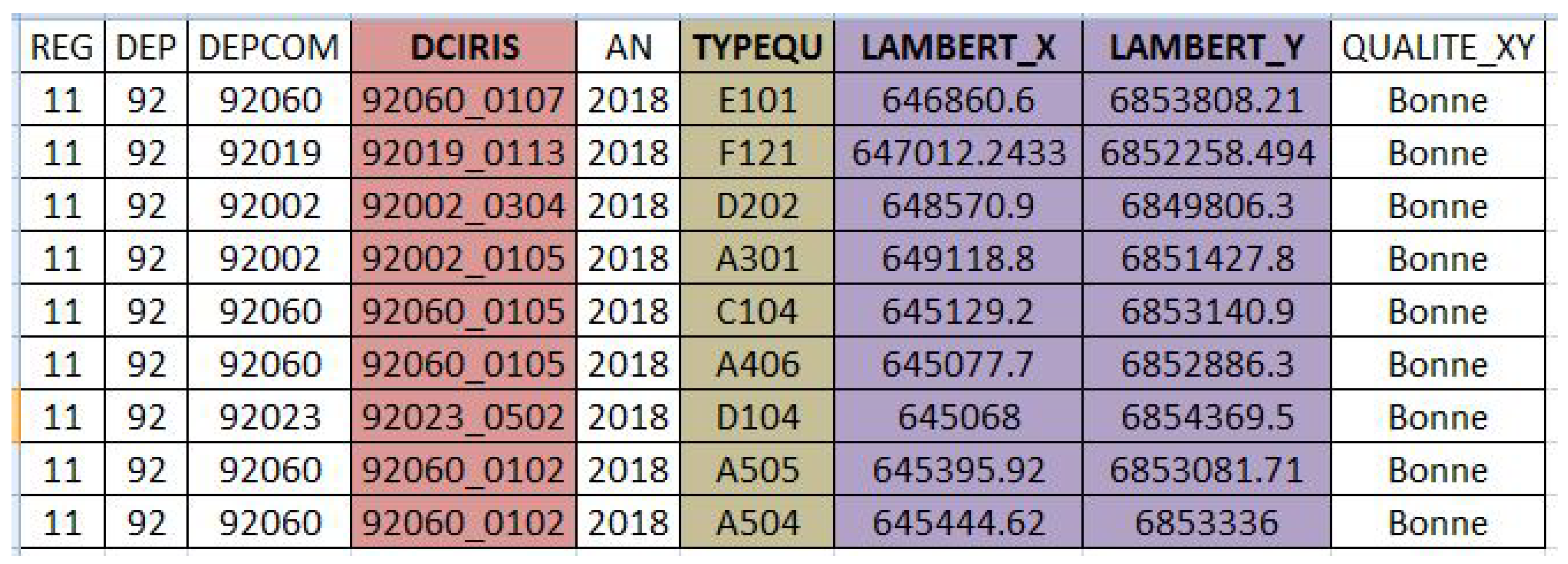
• BPE (Base Permanente des Équipements) intended to provide the level of equipment and services rendered by a territory to the population. This base makes it possible to produce various data about the equipment (indicator of the availability, the density of an item of equipment); all these data being related to a geographical area (IRIS, an equivalent of TAZ Traffic Analysis Zone).
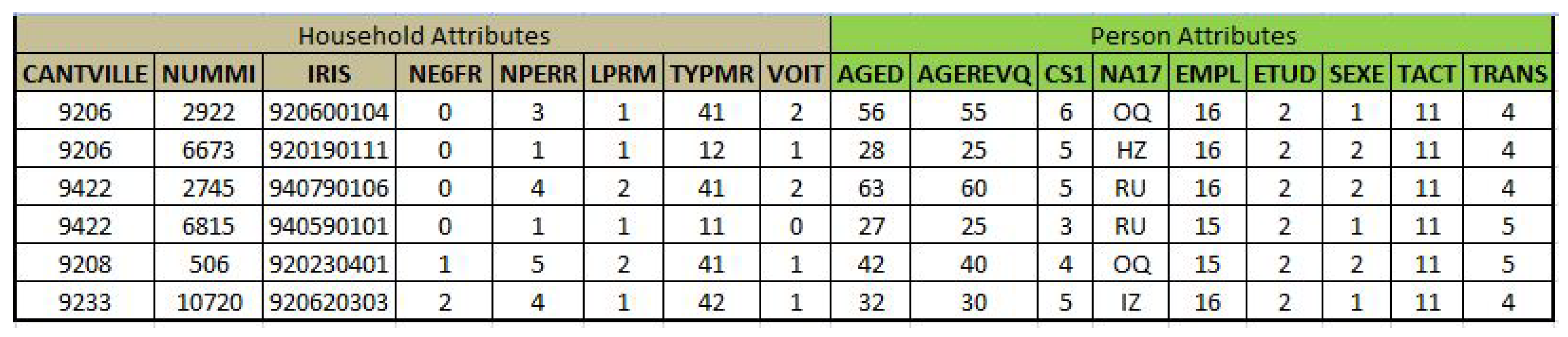
• INDCVI (Individu Localisé au Canton ou VIlle): it is a public census file, it contains an individual-set sorted by the canton Code, each row-data describes an individual (socio-demographic and household characteristics).
• MOB-PRO (Mobilité Professionnelle): bi-localized home-work (trip) data it describing the characteristics of the individual, its household and main residence; the data are sorted by (residence-commune and work-commune).

BPE (Permanent Equipment Base):

BPE [30] file is illustrated in Figure 5: it contains information about the different activity locations, sorted by IRIS zones. The main attributes are presented as follows:

• DEPCOM: Department-Municipality code
• DCIRIS: Commune-IRIS-Code.
• TYPEQU: Equipment type.
• LAMBERT-X, LAMBERT-Y: Activity location coordinates.

INDCVI (Individual Located in Canton or City)

INDCVI (Individus localisés au canton-ou-ville), contains a set of individuals regrouped by canton-ID (CANTVILLE) and household-Number (NUMMI). The national file contains 88 variables for 19,908,607 observations [13]. This file contains several information related to both household and person attributes, in our study, we focused only on an attribute-set detailed in Figure 6 and Figure 7.

MOB-PRO (Professional Mobility)

MOB-PRO (Professional mobility of individuals), in this file, each individual is represented by an attribute-set, the main residence-municipality (COMMUNE), the work-municipality (DCLT). It is related to the working individuals aged 15 years or more, the national file contains 32 variables for 8,074,645 individuals [34]. A section of this file is presented in Figure A1 of the Appendix A.

Study Region: the Catchment Area of LaVallée

Our study (selected) region covers the nearby towns of: Châtenay-Malabry, Le Plessis-Robinson, Sceaux, several TAZ-zones of Antony and Clamart. Figure 8 shows this catchment area, as well as the partition in IRIS zone (TAZ).

4.2.2. Data Processing

Load Activities

Using the main BPE file (2018) [30], we picked the only activities that belong to the selected region (based on the DEPCOM). Then, we translate the geographical coordinates from (LAMBERT-X, LAMBERT-Y) to (Longitude, Latitude). A set of activities is selected to extract their places: (shopping, education, nursery and work). Then, the activities are divided into several classes illustrated in Figure 9 (and Figure A2 of the Appendix A) as follows:

• Shopping: small and large areas.
• Education: primary, middle school, high school and university.
• Nursery: kindergarten and creche.
• Work:

  -

  GZ: Business sector.

  -

  IZ: Accommodation and catering sector.

  -

  JZ: Information and communication sector.

  -

  KZ: Financial and insurance activities sector.

  -

  LZ: Real-estate activities sector.

The activity places for: (home and leisure) are extracted from the OSM file (of the selected region). The activities are referenced by id, classified by type and IRIS zone.

Load Individuals

From INDCVI file, all individuals belong to IRIS zones (TAZ) of selected region are registered (see Figure A3 of the Appendix A).

Integrate Workplace

The aim of this step is to integrate the workplace for the active employed individuals (from selected region) (see Figure 10). For that, individuals from the professional mobility file (MOB-PRO) are loaded for the following cities: Châtenay-Malabry, Le Plessis-Robinson, Sceaux, Antony and Clamart; then, each individual is searched for in the mobility file (MOB-PRO), once found he is assigned a work-city (DCLT) (cf. Figure A4 of the Appendix A). This process is applied only for individuals that satisfied the following constraints:

• Active work status (TACT = “11”).
• Individuals with age equals or more than 18 (AGED > 18).

Assignment Process

The objective of this process is to assign each individual from INDVs (selected region) a workplace (DCLT-attribute), to achieve that, we have first to find this individual (or a similar to it) in MOB-PRO individual-set ($MOBs$). To compare between the individuals, we focus only on the common attributes between MOB-PRO and INDCVI files. The comparison-set (S) contains: AGEREVQ, CS1, EMPL, LPRM, NPERR, SEXE, TRANS, TYPMR and VOIT.

For each attribute ($att$), a factor value (f) is assigned, this factor (see

Table 4. Attributes factors (example).

Attribute	TYPMR	SEXE	LRPM	TRANS	NPERR	EMPL	VOIT	CS1
Factor	+∞	+∞	2.0	1.5	0.8	0.6	0.2	0.2

) represents the attribute-importance (factor-set (F) where $\left|S\right|$ = $\left|F\right|$). We define a parameter called “assignment maximum allowed distance” (M). We assign a mobility person (p) to an individual ($idv$) only if the distance $distance(p,idv)\le M$. The process can be represented as a loop: Assign for each ($idv$) from ($INDVs$), its nearest element ($p_{Near}$) from ($MOBs$) (cf. Equation (2)) only if (M) constraint is satisfied, then the assigned element is removed. At the end of the assignment, M is increased. The process terminates if:

• $C1$: All individuals are updated (work-activity place assigned).
• $C2$: A maximum distance ($maxDistance$) is achieved ($M\ge maxDistance$).

For the individuals that we could not assign for them a workplace (due the constraint $C2$), we set DCLT to undefined value $“?”$.

The method-parameters can be presented as follows:

• $att$: an attribute.
• S: Comparing attribute-set.
• f: an attribute factor, ($f>0$).
• F: Attribute factor-set.
• $INDVs$: Individual-set.
• $idv$: Individual belongs to $INDVs$ ($idv\in INDVs$).
• $MOBs$: Mobility individuals.
• p: Mobility person belongs to $MOBs$ ($p\in MOBs$).
• M: Assignment maximum allowed distance.
• $maxDistance$: Process stop condition ($M\le maxDistance$).
• $H(v1,v2)$: Hamming distance between two values $v1$ and $v2$.

$$distance(p,idv)=\sum _{att\in S}\left(F_{att}·H(p^{att},id{v}^{att})\right)$$

(1)

$$p_{Near}=\underset{p\in MOBs}{min}\left(distance(p,idv)\right)\le M$$

(2)

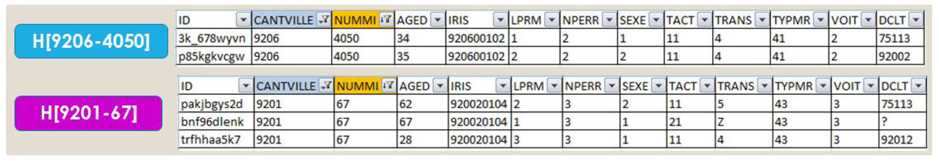
Group Individuals on Households

Individuals are grouped based on (NUMMI and CANTVILLE) attributes (cf. Figure 11).

4.2.3. Activity Plans Generation

Generate Initial Plans

We generate the plans based on the household-members, initially, we consider the following trip purposes (as initial plans) illustrated in Figure 12:

• Home-Work-Home [H-W-H]: for individuals with TACT = “11”.
• Home-Nursery-Work-Nursery-Home [H-N-W-N-H]: for worker parent with children under 6 (NE6FR > 0 and TACT = “11”). In the parent has not an active work status (TACT ≠ “11”), the trip is replaced by Home-Nursery-Home-Nursery-Home [H-N-H-N-H]. If both parents work, only one will have the nursery-activity.
• Home-Education-Home [H-Ed-H]: this trip concerns the student individuals (ETUD = 1).

For individuals (AGED < 6), no activities-plan is assigned.

Instanced Activities

In this step, we assign for each activity a location (from activity places loaded in Load Activities step), the instantiating depends on the activity type:

• Home: we assign to each household a home-place based on its IRIS zone.
• Work: the workplace assigned depends on the type (NA17) and commune (DCLT) of work.
• Shopping, Nursery and Leisure: we assign to them, the nearest activity place from home-place.
• Education: by basing on the individual age (AGED) and student-status (ETUD $=1$), we select the activity type class:

  -

  Primary: $AGED\in [6-11]$.

  -

  Middle School: $AGED\in [12-14]$.

  -

  High School: $AGED\in [15-17]$.

  -

  University: $AGED\ge 18$.

  As the precedent activities, we assign to this activity, the nearest activity-class place.

Extend Generated Plans

Based on the EGT statistics [32] of

Table 5. EGT trip (target activity) by transport mode.

EGT Trip	Target Activity	Public Transport (pt)	Walk	Bicycle	Car	All
Home-Shopping	Shopping	8%	3%	63%	26%	100%
Home-Leisure	Leisure	21%	3%	45%	31%	100%

over the catchment area, a process was applied to extend the generated plans, by adding two activities: shopping and leisure. The process is explained in the diagram of Figure 13).

To overcome the data limitation (trip-proportion by transport mode on study region), we generalize the trip (home—other activity) proportion by mode to ‘target activity proportion by mode’ (see Table 5).

The process starts by selecting an activity (and transport mode) based on the EGT, once the activity is added to the activity plan, we set it location to undefined (“?”). The process allows several successive activities; however, all activity plans have to end by an home-activity (we check a variable return-home after each insertion of a new activity). The trip-chains automate is presented in Figure 14.

Fill Non-Instanced Activities

The non-instanced activities are the activities with a [$location=‘‘?"$], for each missing activity location. As illustrated by Figure 15, we replaced it by the nearest (from home location) activity location from same type (see Section 4.1.1).

Update Workplaces

In the aim to represent all home-work trips of individuals, we distinguish two workplaces updating-processes:

• Outside region workplaces process: this process concerns individuals who work outside of region (Work-out-Region ‘$W_{ORs}$’), by basing on DCLT-attribute; in this process, we define a set of activity locations on region-borders (Work-Borders ‘$W_{Bs}$’) (see Figure 16), we replace for these individuals, the original workplace ($w_{or}$) by the closest one on the border ($w_{selected}$) according to Equation (3).
• Inside region workplaces process: we focus on the individuals who work inside the region, this process covers two cases:

  -

  Work type missing in BPE: in this case, we assign randomly a workplace from the same work-commune (of DCLT).

  -

  Work locations missing in municipality: it is case, where the work type (NA) locations are missing in the selected commune (DCLT). To fix this issue, we update the default workplace by the nearest workplace ($w_{Near}$) from home location ($home$) and belong to the same type (NA) according to Equation (4).

The workplace-updating process parameters can be presented as follows:

• $w_{in}$: workplace in the region.
• $w_{or}$: original workplace (outside of region).
• $w_b$: work-border place.
• $home$: individual home location.
• $W_{ORs}$: Workplaces outside of region.
• $W_{Bs}$: Workplaces on borders.
• $W_{NA}$: Workplaces with $type=NA$.

$$w_{selected}=arg\underset{w_b\in W_{Bs}}{min}\left(distance(home,w_b)+distance(w_b,w_{or})\right)$$

(3)

$$w_{Near,NA}=arg\underset{w_{in}\in W_{NA}}{min}\left(distance(home,w_{in})\right)$$

(4)

5. Discussion

Our modeling shares several common points with previous studies on activity-based modeling and population synthesis generation. However, several distinguishing features are present in our model. First, models usually generate a generic synthetic population for several uses, ending at the household level. In this study, the synthetic population is adapted specifically to the mobility case study: The model generates for each person from the household an activity chain, including the activity type, the transport mode between an activity pair and the activity location. Second, the activities in our model are richer than state-of-the-art proposals (e.g., [7]). Finally, our model is detailed and reproducible. It also uses only public data, it can therefore be directly applied for any case study on any French territory. To the best of our knowledge, this is the first detailed proposal of this kind.

6. Urban Experimentation

6.1. Model Validation

Since we did not have access to classical calibration points (i.e., traffic volume measures or local trip census), we calibrated our model on aggregated data by satisfying the following constraints:

• At least a trip for each individual: after applying Extension plans process, few individuals still had no trip, potentially: unemployed, retired and house-(wife/husband) individuals (TACT ∈ {12, 21, 24, 25}). We added a secondary activity (shopping or leisure) for individuals with no trip.
• Satisfy average-trip ($\alpha$) per user of each city, reported in EGT [32]. For instance, for Antony the potential trips-average ($\alpha =3.67$). The synthetic population is fine-tuned as follow: while population average-trips $avg<\alpha$, select randomly an individual (who has less than $\alpha$ trips T ($\left|T\right|<\alpha$), and add to it a secondary activity.

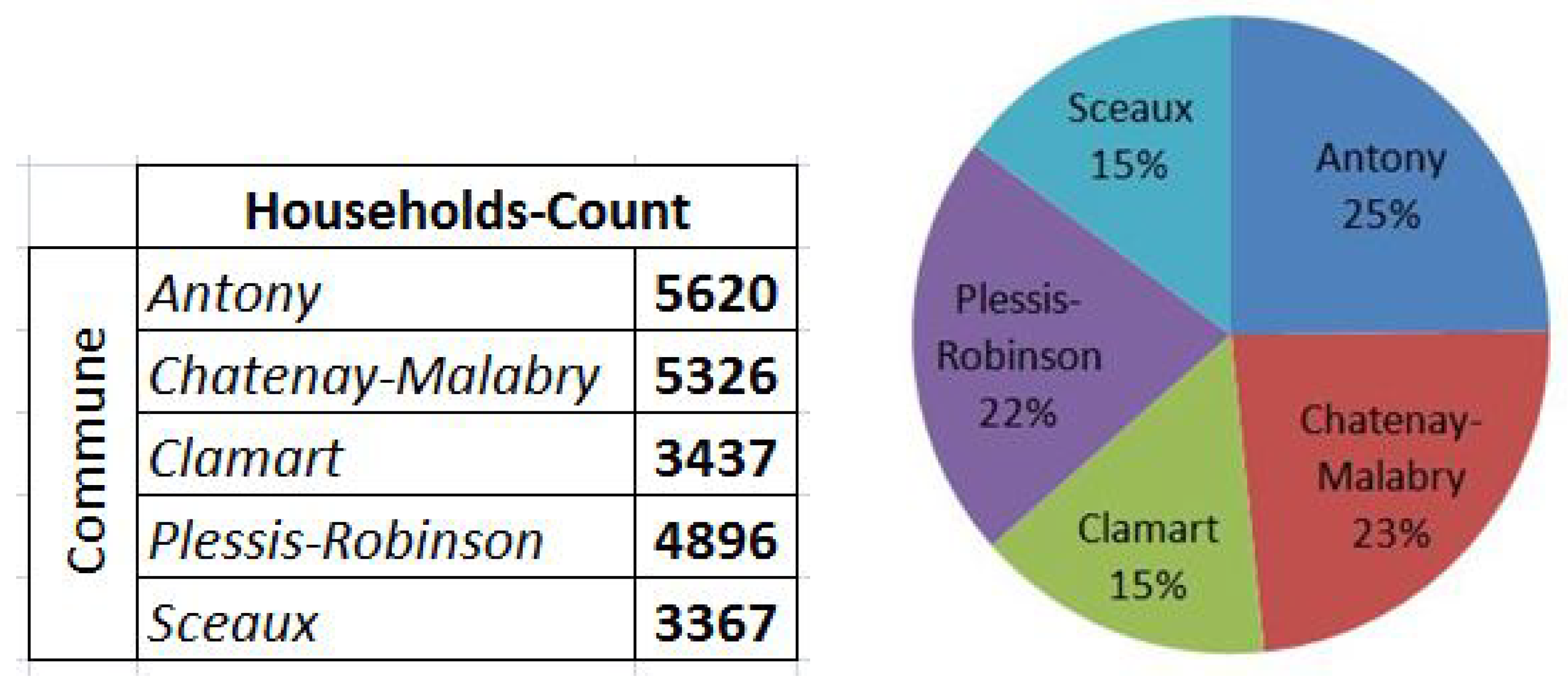
6.2. Composition of the Generated Population

To summarize, we present some statistics about the generated population (and plans). The constructed population is composed of 22,646 households, dispatched over the surrounding cities as described in Figure 17.

Figure 18 describes the generated population in terms of age group. Agents under the age of 18-year-old represent 22% of the population and are mostly busy between education (or kindergarten for toddlers) and leisure/shopping activities.

Individual between 30–50-year-old also have a kindergarten activity since they have to drop off their children to school in the morning and pick them up at the end of the day. People over the age of 65-year-old are mostly busy with leisure and shopping activities for a large share of them are retired.

In Figure 19 are reported transport mode share and activity proportions. Since we have focused on individuals likely to visit LaVallée district, Home is the beginning and end of any travel tour, and this activity represents more than half the trip purposes because some activity chains enables multiple Home leg station.

Figure 20 lists all the activity chains that we have considered in this study. A total of 47,620 plans were devised and are presented in four categories with a variety of possible chains and their total number of plans.

6.3. Experimental Results

As explained in Section 1.2, there are no public data available over the catchment area studied in this article. However, household travel study EGT over the eight departments of Great Paris metropolis are publicly available [32], giving aggregated travel flows with their purpose and mode. Since the region of interest is a sub-region of department 92 (Hauts-de-Seine) as shown in yellow in Figure 1, it is relevant to compare the output of the model with the available travel flows of that specific department, and ensure that they match at least coarsely.

Figure 21 shows a comparison on values of transport mode share for five home-based trip purposes: Education, Kindergarten, Shopping, Leisure and Work. Four transport mode were considered: public transportation, private vehicle, walking and cycling.

At a first glance it can be seen that the travel mode trends are mostly respected between the two areas. A closer inspection reveals however some deviations. Kindergarten mode share is quite accurate (less than 3% error) with 50/45 share between walk and private vehicle which is standard for security matters since it requires accompanying small children to or from the nursery. Shopping and leisure are also well-modeled with a 5% error between walking and car usage.

On the Home-Education trips, public transportation share is close to that of the department according to our model. However, it overestimates of the walk leg of 7% and underestimate the car travel mode for this activity, possibly due to the lack of University in this area (none in this area).

Home-Work trips by walk in the catchment area are close to the share of the department. However, the PT/car share are more coarsely fitted with an 8% and 9% error on public transport and private vehicle mode, respectively. A possible explanation is the remote location of a large part of this area with regards to PT infrastructure and multimodal nodes. Especially Chatenay, Clamart, Plessis and Sceaux cities, which are green areas made of urban districts separated by large parks or parcels of vegetation, and are a little remote to Antony city which has two important multimodal nodes.

However coarse our estimation we still found these figures are accurate enough for our application. Especially if one consider that the 92 department is a rather largely extended area compared to the region of interest, composed of a non-uniform urban fabric with La Defense business district in the North and more Blue-Green infrastructures in the South.

6.4. Travels Patterns and Activity Distribution over the Area

The following videos illustrates the resulting activities and travels over the catchment area:

• www.youtube.com/watch?v=etR4HRBu0Zo shows an overview of the activity location in the catchment area, including home places of the synthetic population.
• www.youtube.com/watch?v=Du3sYPaiQKA shows the dynamic travel model resulting after dynamic traffic assignment of the travel demand using MATSIM. Some planning tours of individuals are also illustrated.

Figure 22 are samples of these videos.

As can be seen in the latter video, a part of the traffic can already be expected in LaVallée district: a vehicle road which shortened the travel time of surrounding travelers.

The next step in this work is now to devise a method to estimate the portion of this foot/car/PT traffic that can be expected inside LaVallée by adding future activity places in the district and adding new plans choices to the individuals.

7. Conclusions

The presented work is part of a larger project that requires estimation of the flow of external visitors of a future district under construction. It is estimated realistically based on the pre-project movements in the areas of influence of the district. In this paper, we technically detailed all steps of a methodology to determine trips and their purpose at a mesoscopic scale including the city and surrounding areas, in the current baseline scenario. We focused on the generation of a synthetic population representative of the current socio-demographic situation of an area of inhabitants prone to be future users of the district. It is built by mobilizing data from census at the departmental level and publicly available land-use data.

Our model is detailed and reproducible, and produces a wide variety of activity plans. To the best of our knowledge, this is the first detailed proposal of the required step to build a set of activity plans. It also uses only public data; it can therefore be directly applied for any case study where such data are available.

The output model is coarse, but it reflects the mobility trends experienced in the department when considering car, public transport, walk and bicycle leg. We could not evaluate the generated population in terms of activity chains, since it would require a specific travel census on the forecasting area. We therefore decided to compare the output with more traditional aggregated travel pattern indicators publicly available in the closest area.

Even with the large number of possible activity chains considered, we found errors of less than 10% on Work and Education trip purposes, and even less for Leisure, Shopping and Kindergarten activity. We argue that the model is still reliable if one considers the only data available for comparisons where aggregated data from a larger area composed of non-uniform urban fabrics.

We believe the method could be useful to practitioners interested in approximate flows and their mode share, when no public travel census is available, or no mean is available to implement one.

References

1. Bonabeau, E. Agent-based modeling: Methods and techniques for simulating human systems. Proc. Natl. Acad. Sci. USA 2002, 99, 7280–7287. [Google Scholar] [CrossRef] [PubMed] [Green Version]
2. McNally, M.G. The four step model. Handb. Transp. Model. 2000, 1, 35–41. [Google Scholar]
3. Jones, P.E.; Koppelman, F.K. Activity analysis: State-of-the-art and future directions. In Developments in Dynamic and Activity-Based Approaches to Travel Analysis; Gower Publishing: Aldershot, UK, 1990; pp. 34–55. [Google Scholar]
4. Smith, L.; Beckman, R.; Baggerly, K. Transims: Transportation Analysis and Simulation System; Technical Report; Los Alamos National Lab.: Los Alamos, NM, USA, 1995. [Google Scholar]
5. Arentze, T.; Timmermans, H. Albatross: A Learning Based Transportation Oriented Simulation System; Eirass: Eindhoven, The Netherlands, 2000. [Google Scholar]
6. Hörl, S.; Balac, M. Reproducible scenarios for agent-based transport simulation: A case study for Paris and Île-de-France. In Arbeitsberichte Verkehrs-und Raumplanung, 1499; IVT: ETH Zurich, Zurich, Switzerland, 2020. [Google Scholar]
7. Dumbliauskas, V.; Grigonis, V. An Empirical Activity Sequence Approach for Travel Behavior Analysis in Vilnius City. Sustainability 2020, 12, 468. [Google Scholar] [CrossRef] [Green Version]
8. Moeckel, R.; Spiekermann, K.; Wegener, M. Creating a synthetic population. In Proceedings of the 8th International Conference on Computers in Urban Planning and Urban Management (CUPUM), Sendhai City, Japan, 27–29 May 2003; pp. 1–18. [Google Scholar]
9. Huynh, N.N.; Cao, V.; Wickramasuriya Denagamage, R.; Berryman, M.; Perez, P.; Barthelemy, J. An agent based model for the simulation of road traffic and transport demand in a Sydney metropolitan area. Fac. Eng. Inf. Sci. 2014. [Google Scholar] [CrossRef]
10. Baghestani, A.; Tayarani, M.; Allahviranloo, M.; Gao, H.O. Evaluating the Traffic and Emissions Impacts of Congestion Pricing in New York City. Sustainability 2020, 12, 3655. [Google Scholar] [CrossRef]
11. Yang, Y.; Atkinson, P.; Ettema, D. Individual space-time activity-based modelling of infectious disease transmission within a city. J. R. Soc. Interface 2008, 5, 759–772. [Google Scholar] [CrossRef] [PubMed] [Green Version]
12. US Census Bureau, American Community Survey. Summary File Data. Available online: https://www.census.gov/programs-surveys/acs/data/summary-file.2015.html (accessed on 12 April 2020).
13. INSEE. National Institute of Statistics and Economic Studies. 2014. Available online: https://insee.fr/fr/accueil (accessed on 6 March 2020).
14. Huang, Z.; Williamson, P. A Comparison of Synthetic Reconstruction and Combinatorial Optimisation Approaches to the Creation of Small-Area Microdata; Department of Geography, University of Liverpool: Liverpool, UK, 2001. [Google Scholar]
15. Guo, J.Y.; Bhat, C.R. Population synthesis for microsimulating travel behavior. Transp. Res. Rec. 2007, 2014, 92–101. [Google Scholar] [CrossRef] [Green Version]
16. US Census Bureau, American Community Survey. 2011–2015 ACS 5-year PUMS Files. 2015. Available online: https://www.census.gov/programs-surveys/acs/data/pums.html (accessed on 7 February 2020).
17. Zhu, Y.; Ferreira, J., Jr. Synthetic population generation at disaggregated spatial scales for land use and transportation microsimulation. Transp. Res. Rec. 2014, 2429, 168–177. [Google Scholar] [CrossRef]
18. Lim, P.P.; Gargett, D. Population synthesis for travel demand forecasting. In Proceedings of the 36th Australasian Transport Research Forum (ATRF), Brisbane, Australia, 2–4 October 2013. [Google Scholar]
19. Metropolis, N. THE BEGINNING of the. Los Alamos Sci. 1987, 15, 125–130. [Google Scholar]
20. Williamson, P.; Birkin, M.; Rees, P.H. The estimation of population microdata by using data from small area statistics and samples of anonymised records. Environ. Plan. A 1998, 30, 785–816. [Google Scholar] [CrossRef]
21. Ye, X.; Konduri, K.; Pendyala, R.M.; Sana, B.; Waddell, P. A methodology to match distributions of both household and person attributes in the generation of synthetic populations. In Proceedings of the 88th Annual Meeting of the Transportation Research Board, Washington, DC, USA, 11–15 January 2009. [Google Scholar]
22. Voas, D.; Williamson, P. An evaluation of the combinatorial optimisation approach to the creation of synthetic microdata. Int. J. Popul. Geogr. 2000, 6, 349–366. [Google Scholar] [CrossRef]
23. Stuart, R.; Peter, N. Artificial Intelligence: A Modern Approach. 2020. Available online: http://aima.cs.berkeley.edu/ (accessed on 15 March 2020).
24. Ranagalage, M.; Estoque, R.C.; Zhang, X.; Murayama, Y. Spatial changes of urban heat island formation in the Colombo District, Sri Lanka: Implications for sustainability planning. Sustainability 2018, 10, 1367. [Google Scholar] [CrossRef] [Green Version]
25. Mauree, D.; Coccolo, S.; Perera, A.T.D.; Nik, V.; Scartezzini, J.L.; Naboni, E. A new framework to evaluate urban design using urban microclimatic modeling in future climatic conditions. Sustainability 2018, 10, 1134. [Google Scholar] [CrossRef] [Green Version]
26. Tillie, N.; Borsboom-van Beurden, J.; Doepel, D.; Aarts, M. Exploring a Stakeholder Based Urban Densification and Greening Agenda for Rotterdam Inner City—Accelerating the Transition to a Liveable Low Carbon City. Sustainability 2018, 10, 1927. [Google Scholar] [CrossRef] [Green Version]
27. Zhao, Y.; Zhang, G.; Lin, T.; Liu, X.; Liu, J.; Lin, M.; Ye, H.; Kong, L. Towards sustainable urban communities: A composite spatial accessibility assessment for residential suitability based on network big data. Sustainability 2018, 10, 4767. [Google Scholar] [CrossRef] [Green Version]
28. Niu, Q.; Wang, Y.; Xia, Y.; Wu, H.; Tang, X. Detailed assessment of the spatial distribution of urban parks according to day and travel mode based on web mapping API: A case study of main parks in Wuhan. Int. J. Environ. Res. Public Health 2018, 15, 1725. [Google Scholar] [CrossRef] [PubMed] [Green Version]
29. Real Time Worldwide Public Transit App. Available online: http://https://moovitapp.com/ (accessed on 8 June 2020).
30. Base Permanente des Equipements (BPE), Institut National de la Statistique et des études économiques (INSEE). Available online: https://www.insee.fr/fr/statistiques/3568656 (accessed on 21 April 2020).
31. Open Street Map. Available online: https://www.openstreetmap.org (accessed on 21 April 2020).
32. Enquête Globale Transport—EGT 2010-Île de France Mobilités-OMNIL-DRIEA. Available online: http://www.omnil.fr/spip.php?article88 (accessed on 21 April 2020).
33. Individus Localisés au Canton-Ou-Ville, INSEE. 2014. Available online: https://www.insee.fr/fr/statistiques/3141862 (accessed on 21 April 2020).
34. Mobilités Professionnelles des Individus, INSEE. 2014. Available online: https://www.insee.fr/fr/statistiques/2866308 (accessed on 22 April 2020).
Figure 1. (Left): Hauts-de-Seine (92) is a 25 km × 15 km department of Paris suburb. (Right): LaVallée district, its catchment area extension with the included cities and their subdivision into TAZ (cartography © INSEE https://www.geoportail.gouv.fr/donnees/iris).
Sustainability 12 05821 g001
Figure 2. (Left): LaVallée: a 500 m × 400 m urban district under construction at present (2020). (Right): digital models of the buildings to be built. Credits: Atelier M3, Arcadis, SEMOP Châtenay-Malabry Parc-Centrale.
Sustainability 12 05821 g002
Figure 3. (Left): the catchment area (15 min accessibility by PC or PT). (Right): LaVallée future road network (legs: walk, bicycle and cars).
Sustainability 12 05821 g003
Figure 4. Global Flowchart: travels and their purposes in the district’s surroundings (exogenous demand) requires first to define a Synthetic Population.
Sustainability 12 05821 g004
Figure 5. BPE file format.
Sustainability 12 05821 g005
Figure 6. INDCVI attributes details.
Sustainability 12 05821 g006
Figure 7. Individuals file format.
Sustainability 12 05821 g007
Figure 8. Selected region surrounding district LaVallée.
Sustainability 12 05821 g008
Figure 9. Selected activity-classes based on BPE.
Sustainability 12 05821 g009
Figure 10. Integrate work-activity flowchart.
Sustainability 12 05821 g010
Figure 11. Grouped individuals on households.
Sustainability 12 05821 g011
Figure 12. Generate initial plans flowchart.
Sustainability 12 05821 g012
Figure 13. Extended plans illustration/flowchart; (Left): example of a plan (home-work-home), select activity/mode (shopping/car), extend the plan by (shopping/car), check the return-to-home (true), adds it (home). (Right): General case.
Sustainability 12 05821 g013
Figure 14. Activity chain automation.
Sustainability 12 05821 g014
Figure 15. Fill none instanced activities flowchart (example).
Sustainability 12 05821 g015
Figure 16. Workplaces on borders (top) and outside of the region of interest (bottom).
Sustainability 12 05821 g016
Figure 17. Resulting households count by city.
Sustainability 12 05821 g017
Figure 18. (Left): Agents distribution by age. (Right): activities realized by each category.
Sustainability 12 05821 g018
Figure 19. Transport Mode and trip purpose share in the district catchment area.
Sustainability 12 05821 g019
Figure 20. A total of 47,620 agents were assigned an activity plan. Activity chains can be grouped into four categories: education-based for students (primary, middle school, high school, university) work-based for employed individuals, daycare tour (with a mandatory drop off and pick up at the nursery) and leisure/shopping chains.
Sustainability 12 05821 g020
Figure 21. Transportation mode share for different trip purposes. (Left): result extracted from the population model of the catchment area. (Right): data from public household travel census EGT of the whole department 92 [32]. Travel mode shares from the model are similar to the 92 census, to a first approximation.
Sustainability 12 05821 g021
Figure 22. (Left): activity location and legend. Dark area corresponds to uninhabited zone such as park, woods and LaVallée (no resident yet). Home places are in dark blue, workplace in light blue, shopping in yellow. (Right): Travel leg mode legends. With walkers as green dots, private cars as white arrow, PT in yellow.
Sustainability 12 05821 g022