1. Introduction
Nitrate fluxes in the water system due to fertiliser mismanagement create substantial environmental and health issues where, particularly in rural communities, efficient and reliable water treatment processes are not always available [
1]. Reliable monitoring of nitrates is therefore critical to understanding and predicting nutrient runoff and, in turn, poor fertiliser application practices.
Traditional methods rely on time-intensive sampling and analysis processes, usually through surface water samples which are collected and analysed in a laboratory (
Table A1,
Appendix A) [
2,
3]. Real-time nutrient sensors have the potential to generate widespread benefits for agriculture and aquaculture industries, while also providing a rapid source of high-frequency data that can assist in mitigating environmental damage in sensitive areas.
One such method of automation involves the use of high-frequency optical sensors. However, the reliability and potential successes of optical nitrate sensors is understudied and has been questioned previously [
4]. One project relied on real-time sensors for pH, conductance, temperature, turbidity, chlorophyll and dissolved oxygen monitoring in water streams; however, to complete nutrient analyses, manual sampling was required to develop a regression model that could estimate bacterial concentrations [
5]. As a result, the study may have benefited from the use of real-time nutrient sensors due to the potential ability to correlate temporal data with the water quality probe results. Another study implemented real-time monitoring buoys to obtain nutrient data [
6]. While innovative, these data are limited due to the small measurement range of the instrument (0–5 mg L
−1 of NO
3), as well as a maximum autonomous monitoring period of six months [
7].
Currently, there is not a complete acceptance of real-time nutrient sensors for reliable mainstream water quality monitoring [
8]. As a result, this perceived unreliability leads to skepticism, which in turn hinders opportunities for the widespread implementation of real-time nutrient sensors. However, previous studies [
9] have shown that readings from optical sensors can be compensated for optical interferences while simultaneously deployed remotely. As a consequence, there is the potential, through a combination of targeted experiments and data-driven modelling, to improve the reliability of in-situ optical sensors, such as those targeting nitrates. In turn, this would assist in allowing responses to environmental issues to occur in real-time.
Consequently, the overarching goal of this study was to design, construct, calibrate and field test a real-time nitrate measurement instrument to enable high-frequency and remote nitrate monitoring applications to occur in the future. This goal was achieved through a number of research tasks, including comparing the accuracy of a NiCaVis 705 IQ sensor (from YSI, Yellow Springs, OH, USA) to a spectrophotometer, under laboratory conditions. The laboratory experiments also contributed to the second aim, which was to design a compensation model for nitrate optical sensors. Finally, this testing and the subsequent compensation models contributed to the third aim of the study, which was to develop and deploy a mobile monitoring station to obtain and transmit water quality data, especially nitrate data, in real-time and at very high-frequencies (30-minute intervals). The achievement of these three aims contributed to our goal to foster the deployment of reliable real-time nitrate sensors for a range of important applications.
2. Materials and Methods
2.1. Phase I. Laboratory Calibration
To start the development of a mobile monitoring system, a comprehensive laboratory calibration of the NiCaVis 705 IQ sensor was conducted. This sensor specialises in identifying the concentration of several water quality parameters in real-time, at high-frequency intervals. The focus of this particular study was on calibrating its nitrate detection capability [
10]. As a result, the sensor was specifically calibrated to account for the expected waterway conditions of the region, which are likely to differ significantly depending on the location of deployment. However, most rivers tend to share similar water quality ranges; hence, the goal was to develop a compensation range that could make the nitrate readings from NiCaVis reliable and consistent with what is typically observed in these waterbodies [
11,
12].
To achieve this, potassium nitrate solutions with concentrations ranging between 0.05 mg L
−1 and 500 mg L
−1 were created, thus allowing a set of samples capable of simulating eutrophication conditions (concentrations > 2 mg L
−1 [
13]) to be developed, while also enabling the assessment of the efficacy of the NiCaVis 705 IQ sensor through a broad enough concentration spectrum [
14,
15,
16,
17,
18].
The preliminary calibration and analysis was conducted by measuring potassium nitrate solutions with the NiCaVis 705 IQ sensor as well as a laboratory spectrophotometer and comparing the results as a standardisation measurement. Upon developing this baseline for both devices, interference sources consisting of alterations to the pH, salinity, turbidity, humic acid content, bromide content and temperature were made to calibrate the sensor under different conditions, particularly since studies have shown that these parameters may reduce the accuracy of optical sensors [
9,
19,
20,
21,
22]. Thereafter, a repetitive measurement method was followed to obtain the sought-after results. Firstly, 50 mL of potassium nitrate was placed in tubes, where an interference source was applied and thoroughly mixed to create a homogenous solution. Each sample was then analysed by a laboratory spectrophotometer and the NiCaVis 705 IQ, and the results were compared afterwards. Finally, the remaining liquid was discarded, and the process was repeated for the remaining interferences.
Upon completing the laboratory calibration, the data were analysed to validate the sensor’s readings and to develop compensation models as required. In doing so, a multiple regression model was developed to predict real nitrate concentrations based on two input variables (turbidity and raw nitrate readings).
2.2. Phase II. Mobile Trailer Development
The development of the mobile trailer was conceptualised to address some of the issues regarding the accessibility and implementation of traditional water quality monitoring methods. Sampling from rural locations at regular intervals is costly, as is the implementation of methods to maintain the health of the waterways in these isolated areas. Thus, a mobile trailer was considered useful due to its movability to different locations, as well as its capability to remotely transmit nitrate and other water quality data via a cloud-based system, thus eliminating the need for continual trips to rural areas.
However, to develop the trailer, two aspects had to be considered: the exterior casing and the interior space. For the exterior, the aim was to obtain a relatively inexpensive trailer that had the capability to be adapted and modified to suit the project’s needs, while the interior required sufficient spacing to hold two sensors, an analysis container, communications/pumping systems, as well as additional auxiliary electronics.
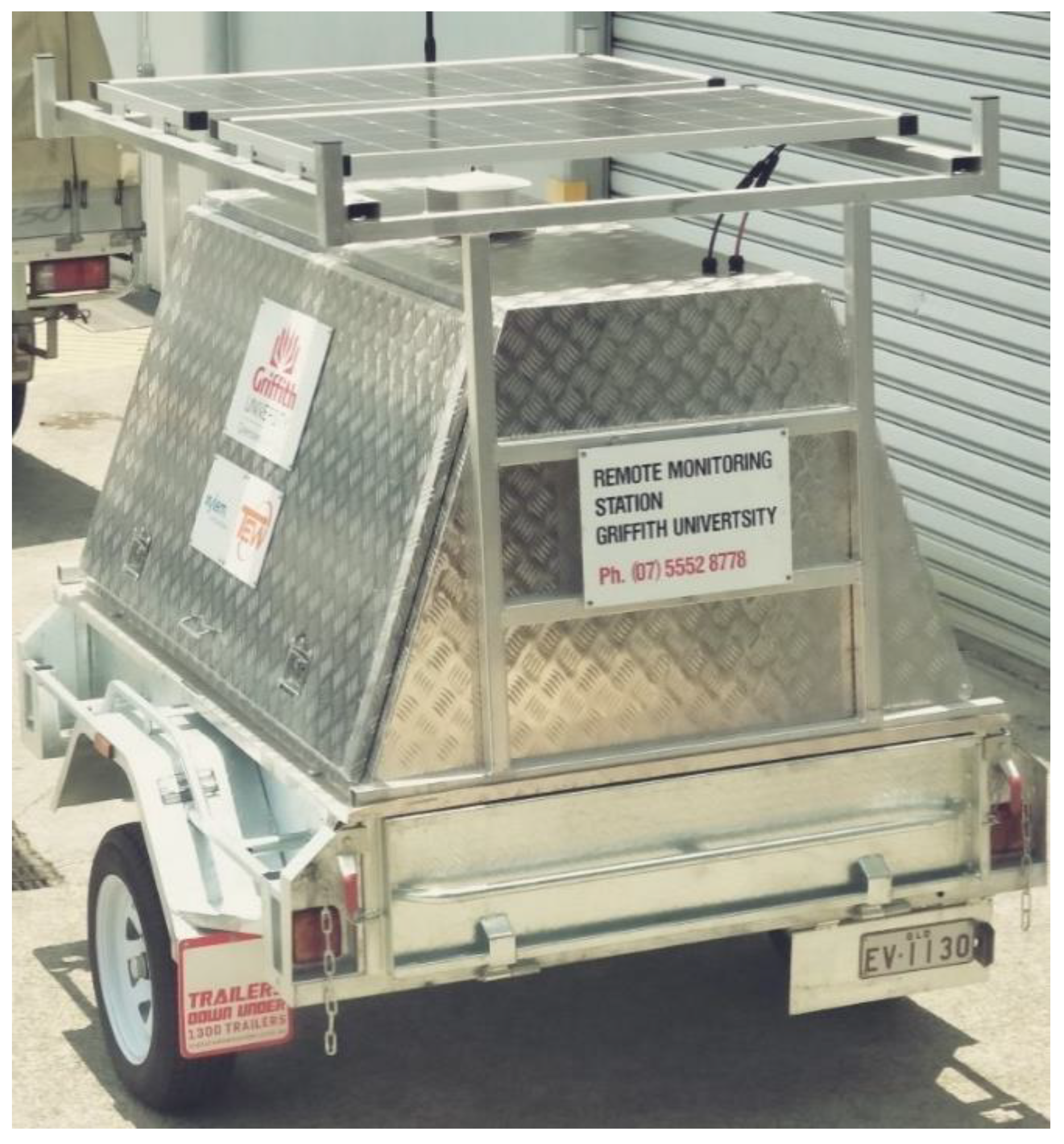
Figure 1 displays the exterior modifications, where solar panels were added to a trailer and connected to batteries to provide sufficient power supply to the system.
Figure 1 also depicts the overall housing for the sensors, where a steel-cased trailer was selected to ensure that a robust, durable system could be setup.
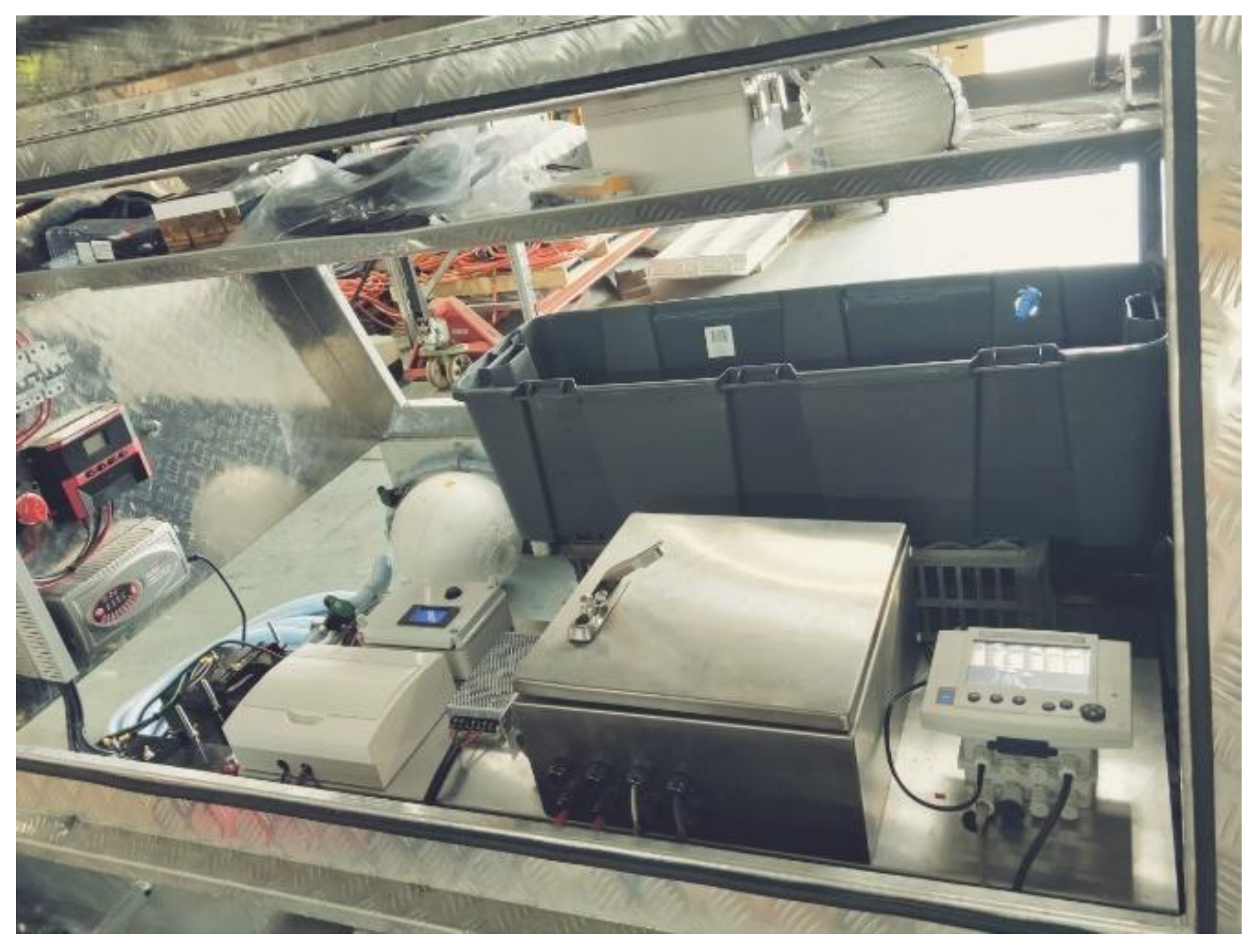
Figure 2 then displays the interior design that was adopted to house the electronics, communication system and sensors.
Overall,
Figure 1 and
Figure 2 display relatively simple housing for the required systems, where an additional compartment was used to store a pumping system. The design of the mobile trailer was created with the intention that the entirety of the water quality monitoring instruments could be held within the one compartment. Therefore, only a small pump had to be placed outside of the trailer to extract water into the wet area, where the sensors could identify the nitrate and water quality parameter concentrations at half-hourly intervals. The data were then streamed through the communications datalogger and automatically uploaded online to a cloud-based server, known as Eagle.IO (
https://eagle.io/). Further details regarding the piping and instrumentation layout are displayed in
Figure A1 of
Appendix B.
Overall, the mobile trailer was designed and constructed to be robust and reliable for field research applications. While the design could be refined further and optimised, the focus of the current study was on its capability and accuracy to remotely collect high frequency water quality parameter data. Future design optimisation work could be conducted on the trailer shelter, water sample pumping system or the renewable energy system, where reduced sizes and capacities could result in cost-savings without compromising operational performance.
2.3. Phase III. Pilot Field Study
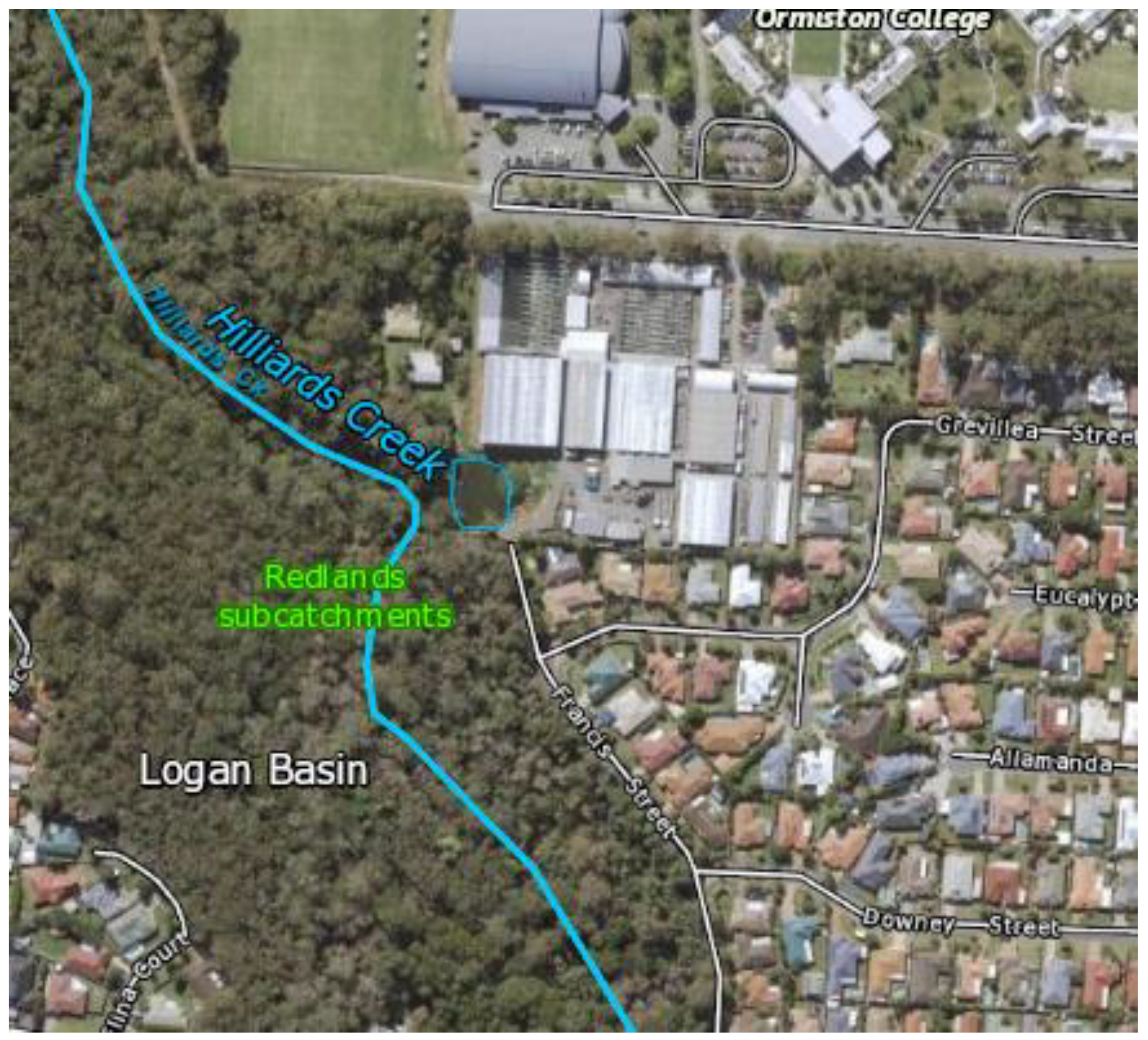
The pilot field study took place at Hilliards Creek in Queensland, Australia. Located in the small town of Ormiston (population < 6000), the site provided an ideal opportunity to test the monitoring trailer in a secure and secluded area.
Figure A2 in
Appendix C displays a map of the pilot location, which was chosen due to the site’s proximity (3.4 km) to an upstream wastewater treatment plant (WWTP). The WWTP is known to discharge nitrate-containing effluent into Hilliards Creek, and hence the location provided the opportunity to achieve this study’s goals by providing a location to collect accurate, high-frequency nitrate data.
In order to collect the water quality data, the sampling pump was placed in the water at approximately 30 cm above the sediment bed. Agrometeorological data were collected at half-hourly intervals, which included nitrate concentrations (from the NiCaVis 705 IQ), as well as the pH, turbidity, salinity and temperature (obtained by Xylem Analytics’ EXO2 Sonde, from YSI, Yellow Springs, OH, USA) of the waterway. Furthermore, rainfall data were obtained at the same frequency from a gauge located adjacent to the WWTP. Prior to the fully automated implementation, the system was calibrated using surface water samples, which were verified with laboratory water quality analyses. The trailer was then left to collect data for nearly four days, before a 1% average exceedance probability (AEP) rain event halted further monitoring due to disruptions from a subsequent flash flood. Despite this, the data were collected through Eagle.IO, where no on-site monitoring was needed after the initial calibration of the equipment.
3. Results
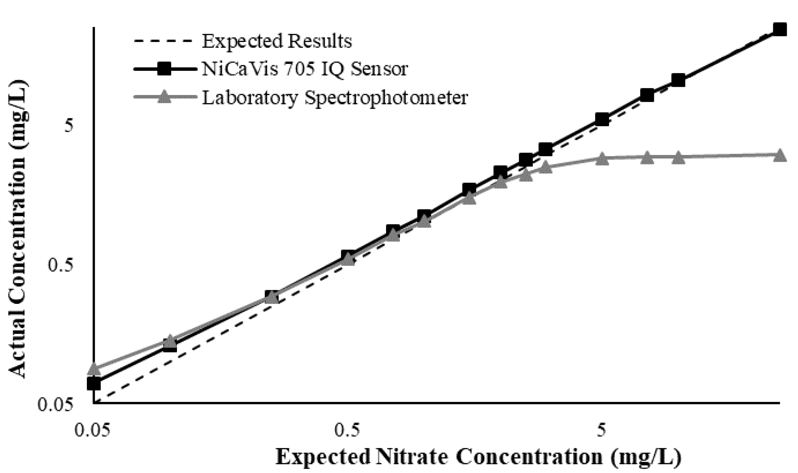
3.1. Phase I. Laboratory Calibration
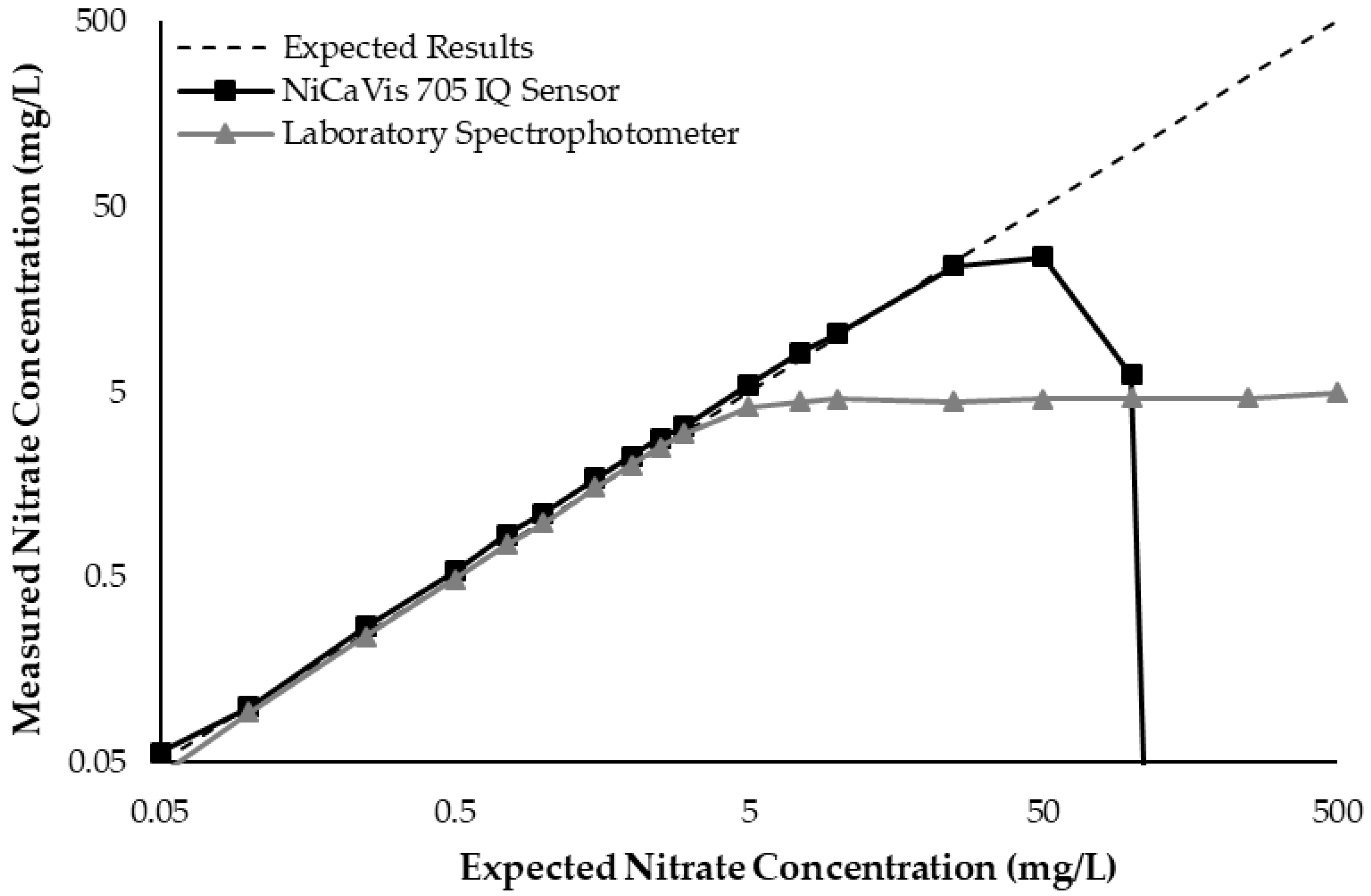
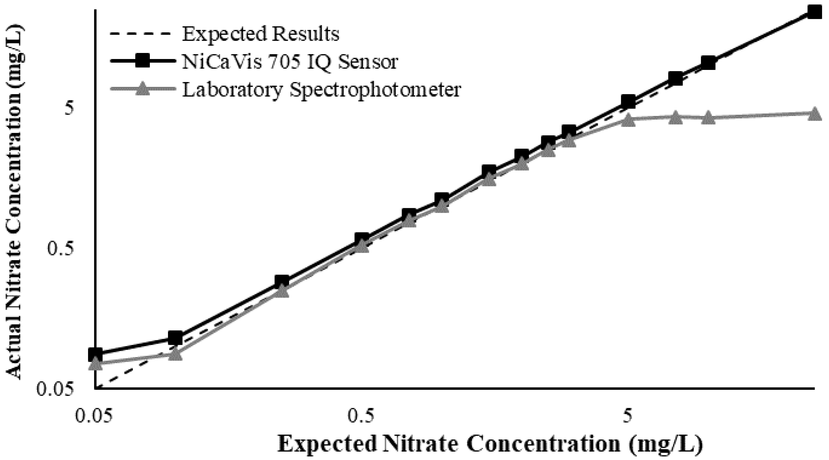
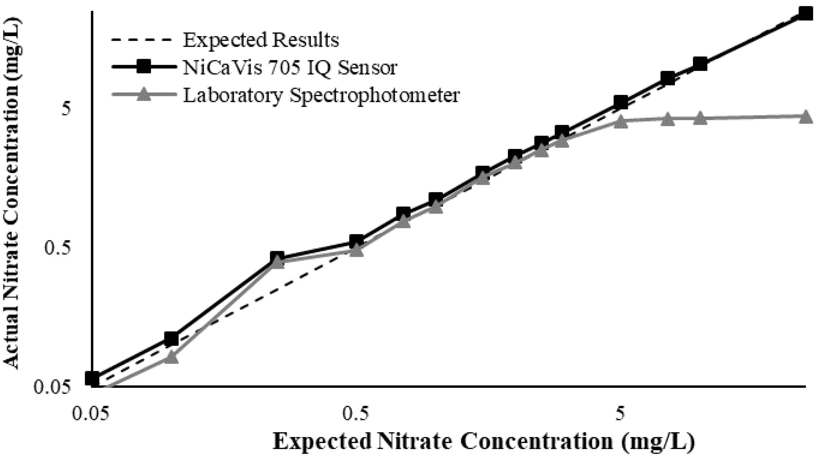
Figure 3 illustrates a comparison between the nitrate readings obtained with the NiCaVis 705 IQ sensor and a laboratory spectrophotometer, for concentrations ranging between 0.05 mg L
−1 and 500 mg L
−1 without interference sources applied.
For the NiCaVis 705 IQ sensor, good accuracy was achieved up to a concentration of 25 mg L
−1, with a rapid drop in accuracy thereafter. The sensor was unable to measure nitrate concentrations beyond 250 mg L
−1. The spectrophotometer was shown to be accurate for nitrate concentrations only up to 3 mg L
−1; readings beyond this showed a constant concentration of 5 mg L
−1. This was believed to have resulted from an Inner Filter Effect (IFE), which occurred as a result of the analyte concentration being too high, causing signal loss in the spectrophotometric analysis [
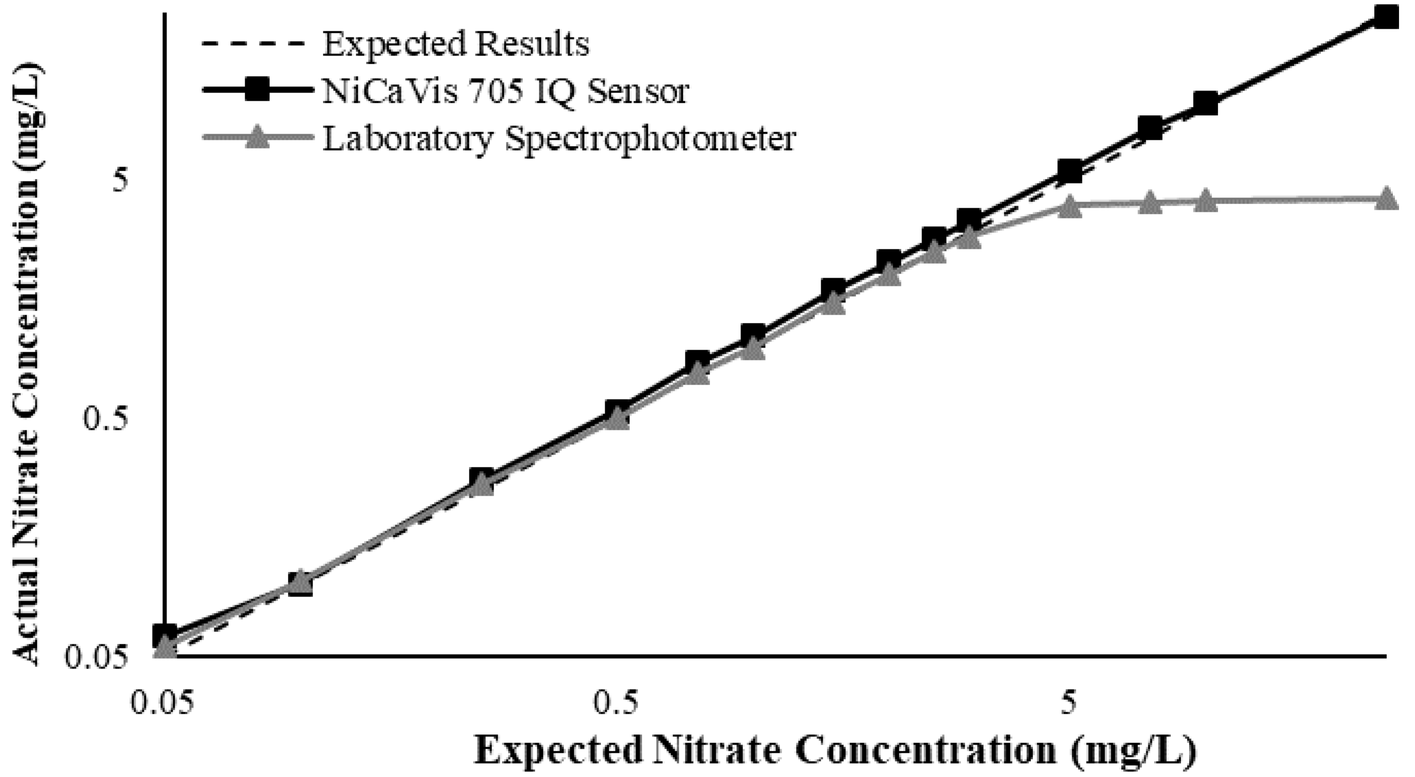
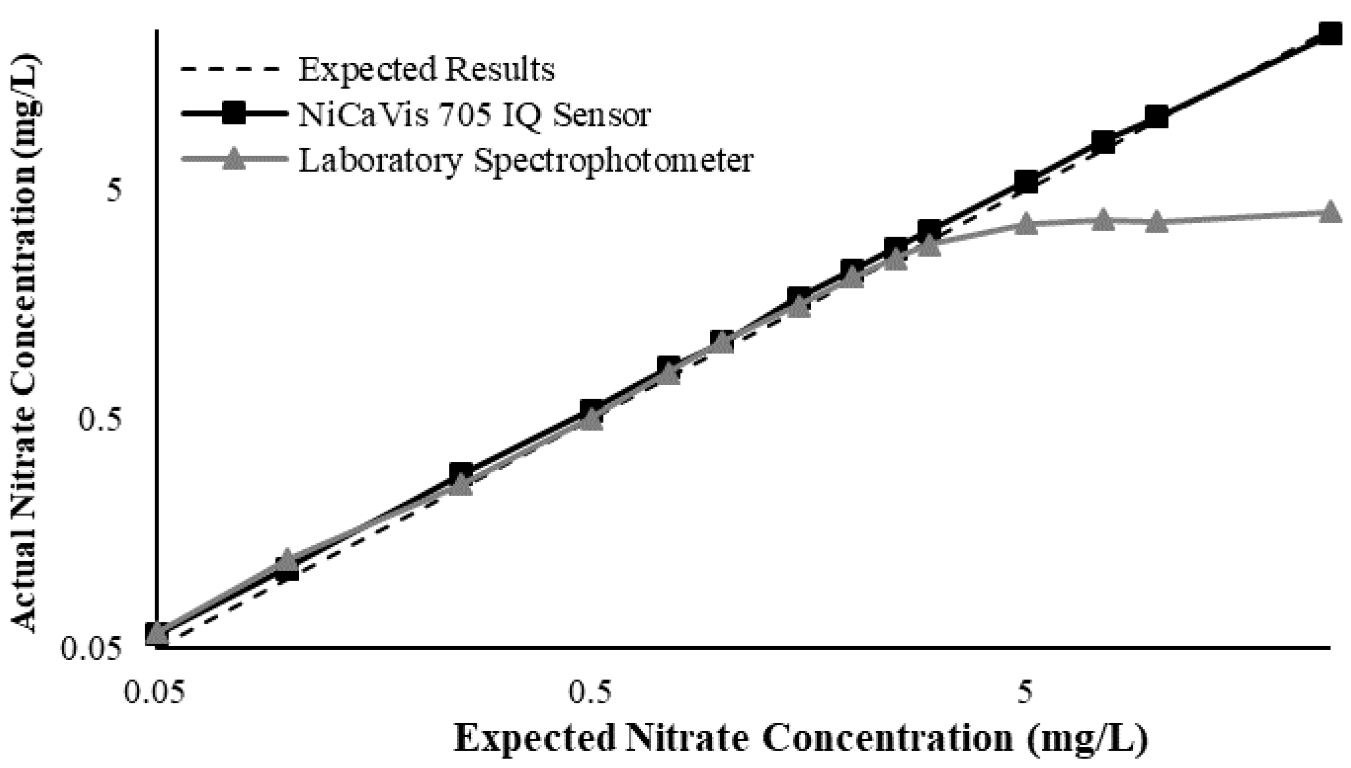
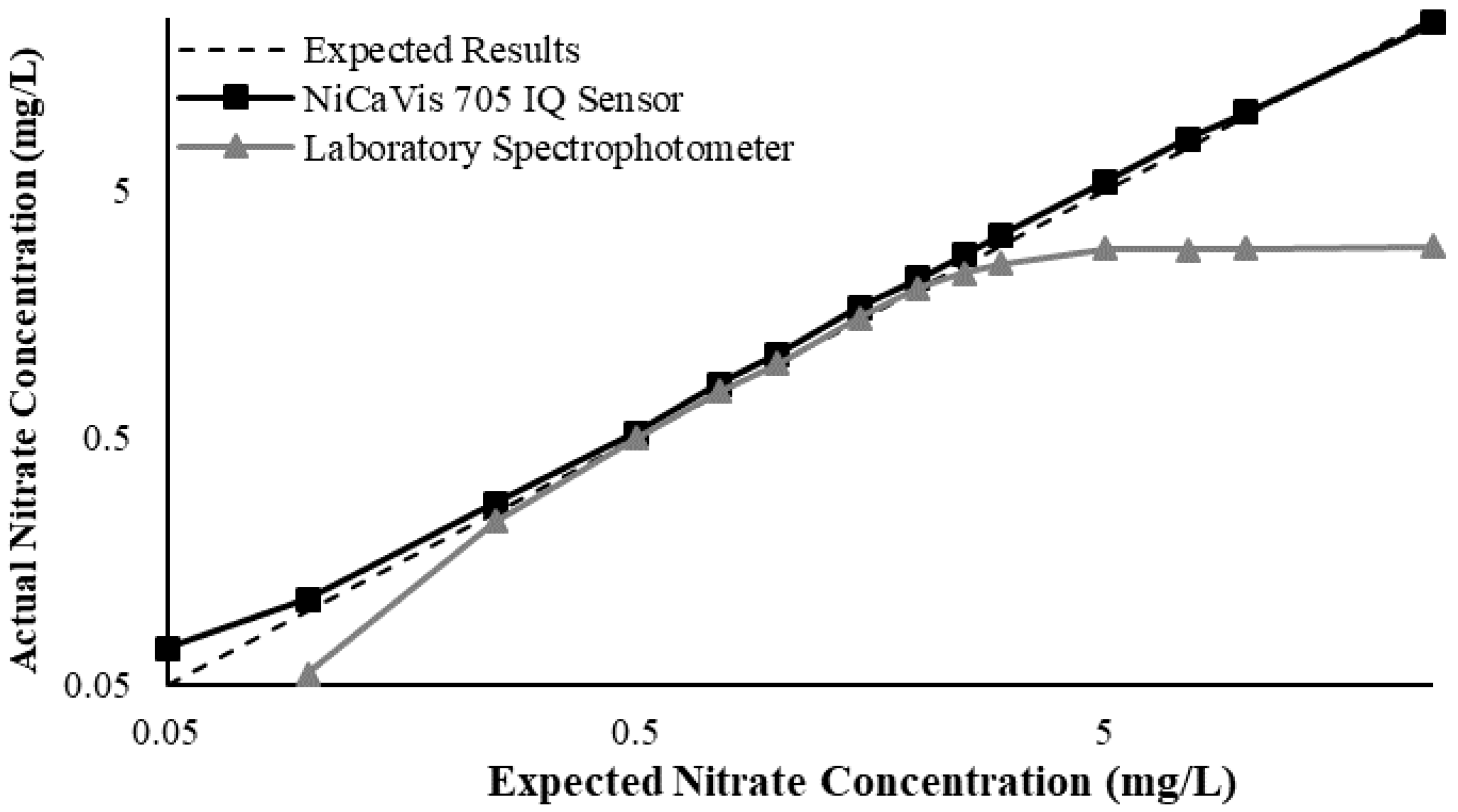
23]. Additional figures to emphasise the performance of the sensor and spectrophotometer when measuring interference sources such as turbidity, pH, temperature, bromide, humic acid and salinity are presented in
Appendix D. The results of these experiments display a similar trend to the one observed in
Figure 3, emphasising the higher accuracy of the sensor when compared with traditional water quality monitoring methods.
Overall, NiCaVis was able to determine concentrations within 0.1 mg L−1 of the baseline in 81% of the samples tested (n = 240), while the spectrophotometer was only able to achieve this in 63% of tests. Furthermore, the sensor read concentrations within a 0.5 mg L−1 range in 96% of cases, while the spectrophotometer had the same result in only 84% of samples. If accounting for the error in samples >5 mg L−1, the number of samples within that range of accuracy decreases to 67%.
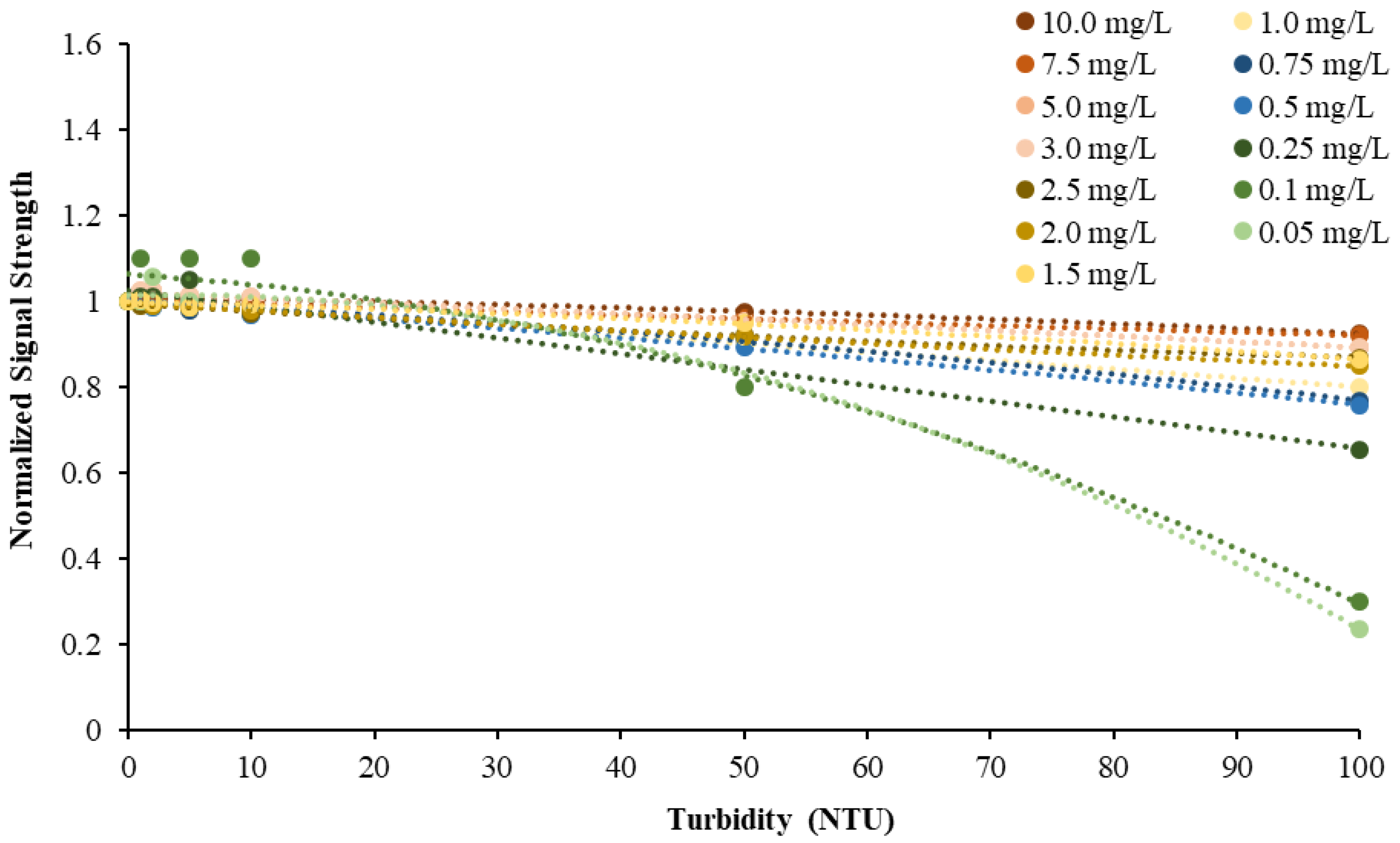
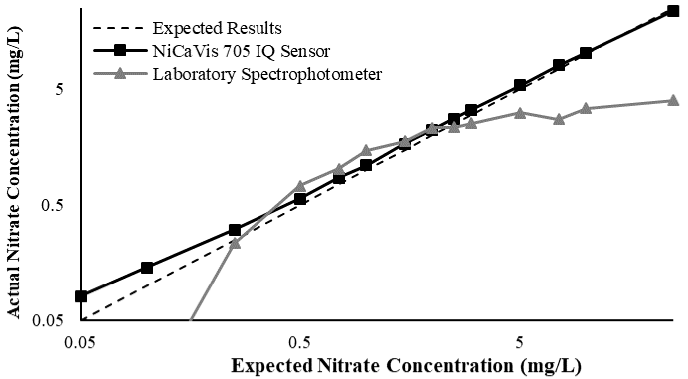
This study also found that the accuracy of NiCaVis can be improved through extensive compensation modelling and reading adjustments. Turbidity was found to be the largest interference source: elevated levels of turbidity with lower nitrate concentrations had the tendency to reduce the sensor’s ability to accurately detect the level of nitrate.
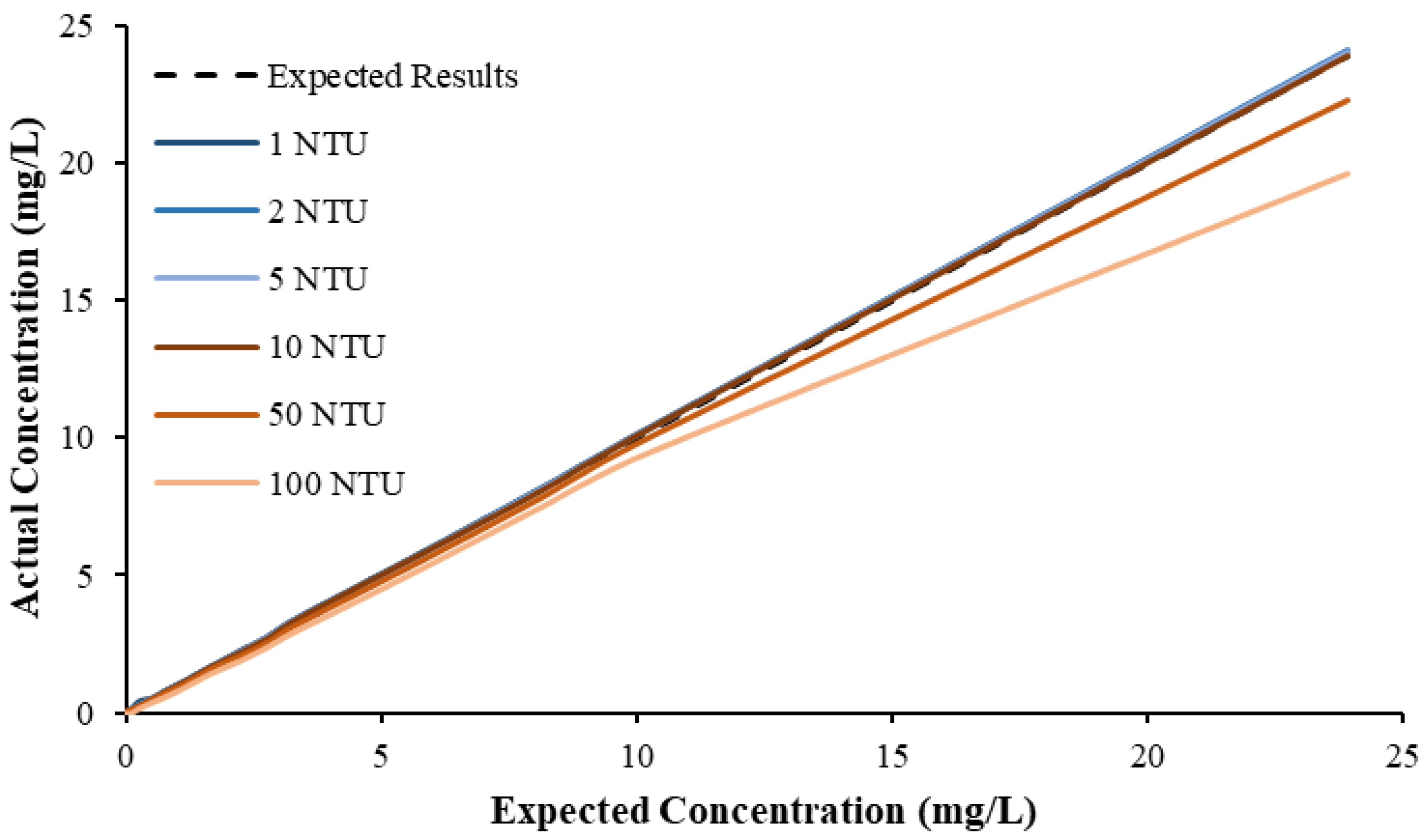
Figure 4 displays this correlation, indicating that a smaller nitrate presence causes a larger signal loss with increasing turbidity.
Figure 5 then displays the relationship between the expected and experimental nitrate concentrations, based on different turbidity levels.
From the above data, a preliminary compensation model was developed, as shown in Equation (1) (
R2 > 0.99).
where [NO
3,A] is the actual corrected nitrate concentration of the sensor, [NO
3,S] is the nitrate concentration read by the sensor and Tb is the turbidity of the waterbody.
This research found that there were limitations to the model, and hence further analyses would be necessary to reinforce the validity of interference compensations, while additional studies could help to develop more complex threshold models to better determine the corrected nitrate reading based on more refined intervals. Regardless, the model was practical in correcting erroneous results for nitrate concentrations >0.1 mg L
−1; however, significant inaccuracies were noted for lower concentrations. Despite this, the likelihood of having concentrations <0.1 mg L
−1 in farmland rivers or creeks susceptible to nutrient releases is low, which is evidenced by the real-time data collected during the pilot study (
Figure 6).
3.2. Phase II and III. Mobile Trailer Development and Pilot Field Study
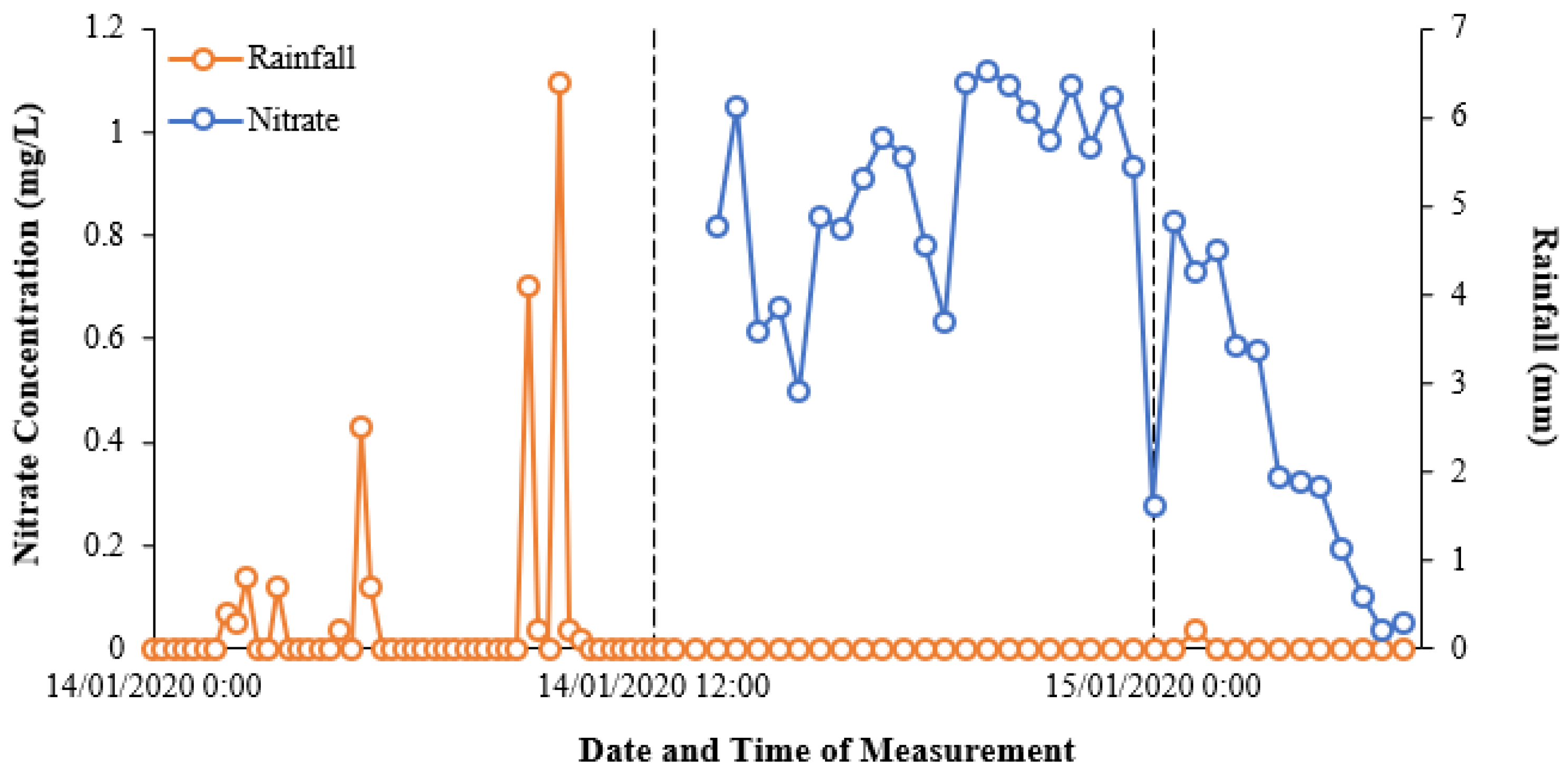
Figure 6 shows the initial relationship between nitrate concentrations and rainfall over the pilot study monitoring period, based on the data extracted from Eagle.IO.
Figure A20 in
Appendix E displays the virtual graphing interface that the software uses to visualise readings collected by the sensors.
Figure 6 highlights the nitrate–rainfall correlation for the operational cycle of the NiCaVis sensor until it was turned off for maintenance. Furthermore, approximately 12 hours of rainfall preceding the NiCaVis’ commencement of recording data is also shown.
The data seem to show that rainfall events caused delayed decreases in nitrate concentrations due to the dilution of water entering the creek. Such a delayed dilution effect was expected due to the inherent processes involved with runoff generation following rainfall, as well as flow movement downstream. In addition, given that the location of the rainfall gauge is 3.4 km upstream from the trailer deployment site, this further emphasised why the delay between rainfall and nitrate readings existed. Although the lack of nitrate data for the 14th of January does not allow us to validate such claims, the dilution effect portrayed in
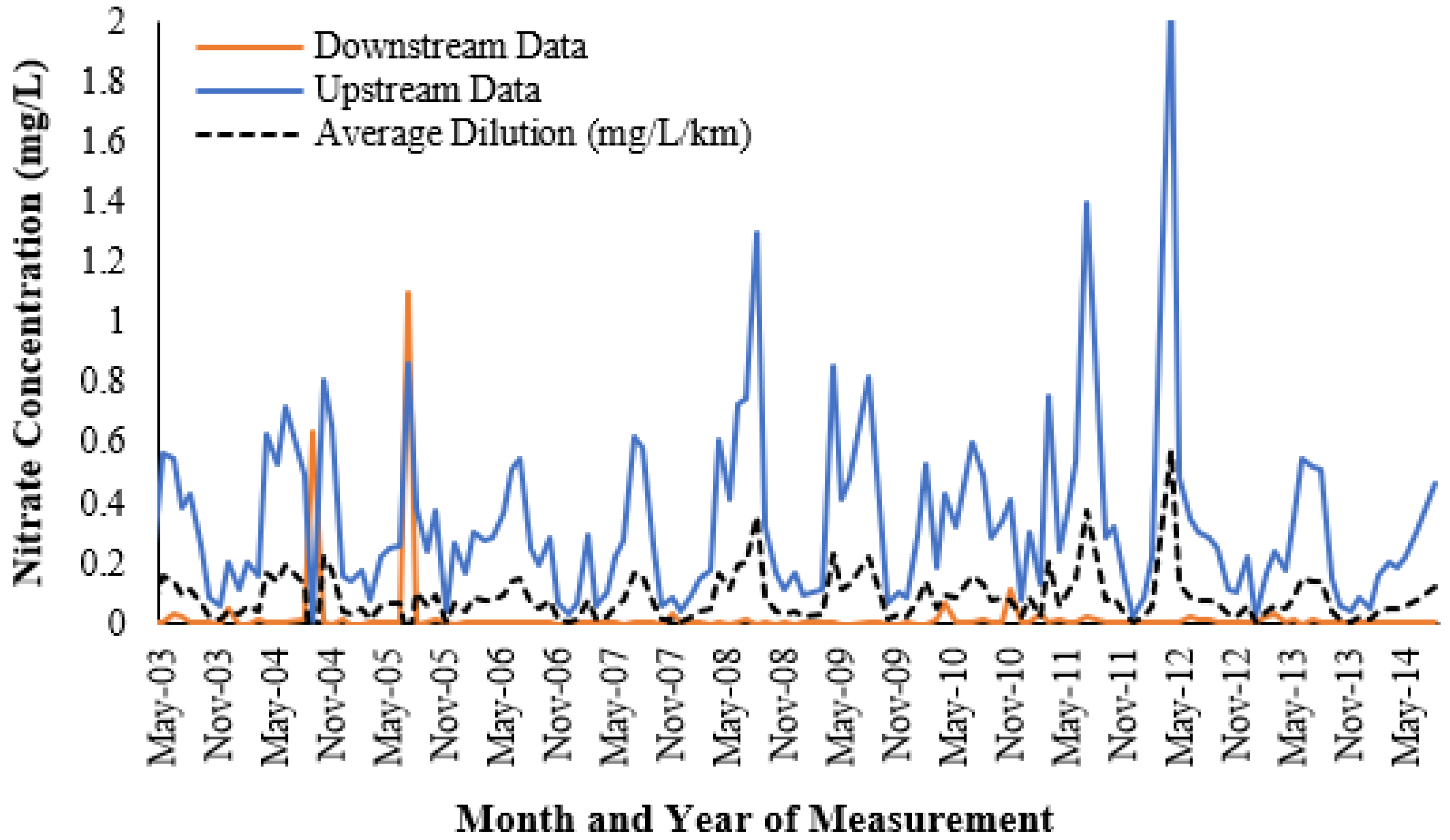
Figure 6 is also supported historically, with
Figure 7 showing the variation of nitrate concentrations that have occurred seasonally from 2003 to 2014.
Figure 7 displays an evident trend where nitrate concentrations had the tendency to lower significantly during the wet season (November to April) and rise during drier periods. Therefore, this data supports the results observed in
Figure 6, displaying the inverse correlation between rainfall volume and nitrate concentration in waterways.
In addition,
Figure 7 also presents a significant difference between the nitrate concentrations at Hilliards Creek (recorded 200 metres downstream from the current study) and at a location further downstream (3.61 km away). As a result, comparing the historical monthly upstream data to the results highlighted in
Figure 6 indicates that an inflow source (the WWTP) was causing significant increases in nitrate concentrations, which then diluted downstream.
Furthermore, the variation of the data in
Figure 6 also emphasises the necessity of real-time and high-frequency nutrient monitoring as significant variations are possible in short timespans. The data in
Figure 7 show significant historical variations on a monthly basis and hence indicates that the typical sampling frequency (i.e., monthly) used for monitoring is unlikely to be truly representative of a waterway’s health or of shorter-term nutrient fluctuations, which appear to occur.
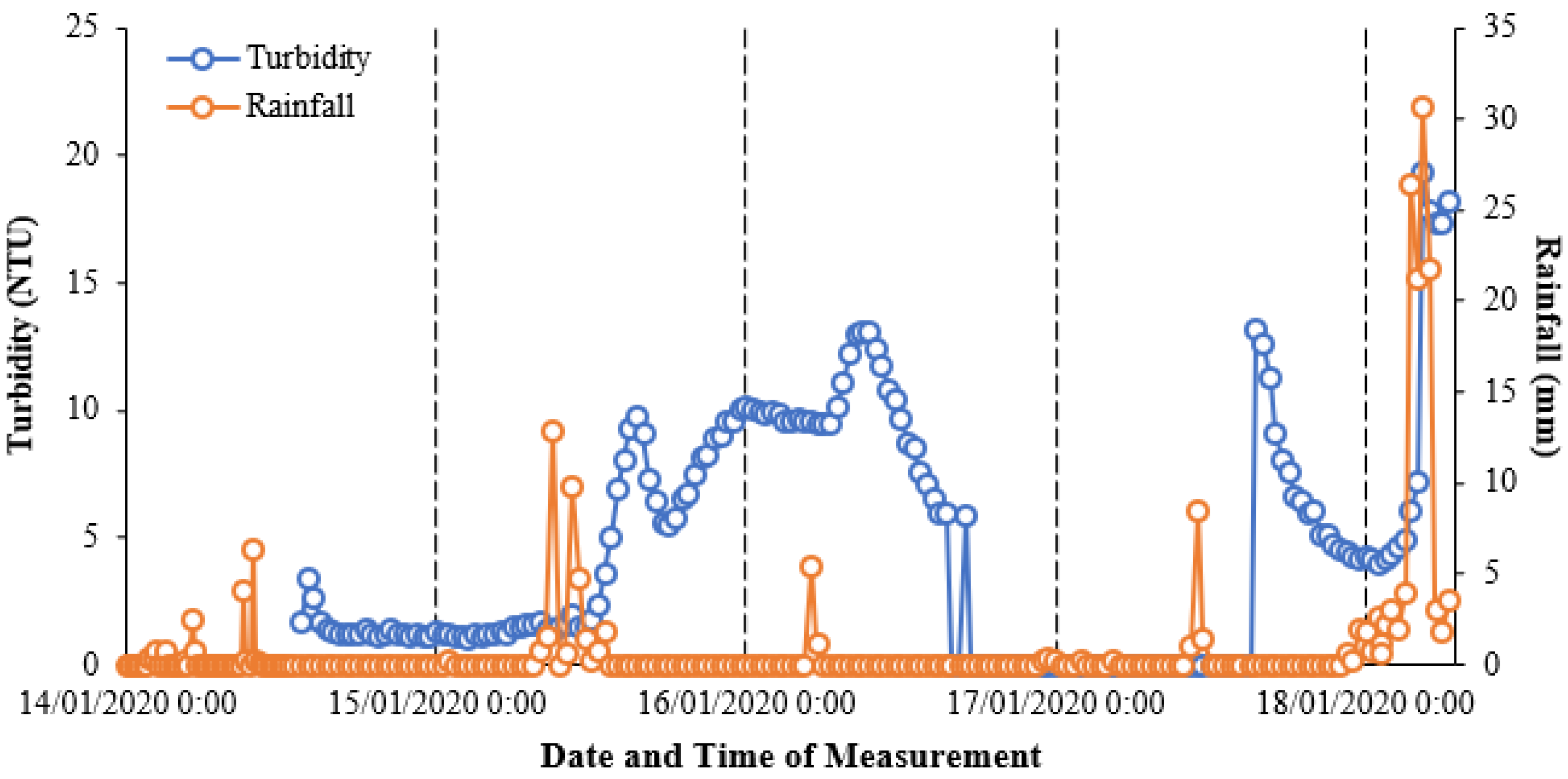
Figure 8 displays the turbidity data collected by the Xylem Analytics’ EXO2 Sonde, coupled with rainfall data.
The correlation between preceding rainfall and turbidity is evident due to a lag of eight hours between the commencement of the rainfall event and the first increase in turbidity. In addition to causing an optical interference on nitrate readings, it is possible that more turbid waters may reduce the ability of chlorophyll-
a to absorb energy from the sun, in turn reducing algal blooms and preventing nutrient uptake [
24]; hence, simultaneous monitoring of turbidity and nitrates is critical for accuracy. Further analyses would be required to affirm this correlation; however, collecting more consistent nitrate, chlorophyll-
a, turbidity and rainfall data could reveal some patterns that may be modelled and integrated into future studies to predict and manage the physicochemical conditions of waterways.
At 5:30PM on 16/01/2020, the mobile trailer system was turned off to complete operational maintenance. When the system was re-established, a significant rainfall event occurred afterwards, thus allowing further correlations to be made, as illustrated by the data presented after 12:30PM on 17/01/2020. Consequently,
Figure 8 displays significant turbidity rise associated with the overnight rainfall event that occurred between 3:00AM and 5:00AM on January 18, 2020. This sudden and large burst of precipitation, noted as a one-in-100-year event, caused an increase in turbidity from 1.3 NTU (which was the base level detected with no preceding rainfall), to 19.33 NTU, an almost 15-fold increase. However, due to the severity of this event, elevated creek levels occurred such that the mobile system was inoperable for several days thereafter.
Despite this, the data presented in
Figure 8 showed that rainfall events, particularly those of large magnitudes, may cause significant elevations in turbidity, and hence the data would require compensating to ensure that the readings made by the NiCaVis 705 IQ sensor and its auxiliary units are maintained at an accurate level.
4. Discussion
The completion of the pilot study consisting of laboratory calibrations and compensation modelling, as well as the trailer development and its subsequent deployment, has the potential to provide numerous benefits. The advantages of obtaining high-frequency nutrient data were explored in this study, where the 30-minute interval results provided the opportunity to observe the highly dynamic nature of water quality parameters. Consequently, the next sections briefly discuss the potential applications of the mobile trailer, as well as the implications of collecting data at a high frequency over long time-periods.
4.1. Agricultural Benefits in Rural Regions
The overproduction of crops to meet increased food demand has caused increases in fertiliser usage, leading to significant environmental damage and exemplifying the need for real-time, remote monitoring at vulnerable waterways. For lower socioeconomic nations, such as those within the tropics, routine monitoring through traditional methods is not feasible due to their diminished capability to proportionately improve their agriculture production [
25]. As a result, countries in the tropics are struggling to implement monitoring regimes that can mitigate environmental harm and minimise economic losses from mismanaged fertiliser usage. Thus, one such application of a real-time, high-frequency system for water quality monitoring is to provide vulnerable nations with a way to continually monitor agricultural effluent. In doing so, fertiliser runoff can be effectively managed using real-time monitoring, thus providing an option to assist decision-makers in the reduction of economic losses associated with high-volume discharges.
4.2. Minimisation of Nutrient Pollution from Aquaculture Practices
Aquaculture industries pose a significant threat to waterway health. In recent years, nutrient inputs have significantly declined, with the conversion efficiency to assist in the growth of aquatic organisms also improving [
26]. However, excretion products from these organisms persist and have the potential to cause significant environmental and ecosystem changes. This therefore presents issues where excess nutrient loads can not only lead to eutrophication but can cause disruptions to marine species. One study [
27] found that up to 45% of nitrogen provided as a food source could be excreted by some organisms, emphasising the significant detriment that mass aquaculture production may have on water quality. Therefore, real-time, high-frequency monitoring can be applied to better equip stakeholders to manage effluent releases into general waterways. In doing so, the timing and volume of nutrient-rich discharge can be managed to provide a lower overall threat to waterways and ecosystems.
4.3. Improvement of Environmental Health in Environmentally Sensitive Areas
As previously mentioned, traditional water quality data are usually obtained, analysed and reported at monthly intervals. This minimises labour and technological costs while also providing relatively accurate results regarding the health of waterways. However, this study has highlighted that the overall complexity of river/creek systems is high, with the dynamic nature of these systems causing large fluctuations of physicochemical and nutrient concentrations in short time-periods. For typical waterbodies, the importance of measuring the significance of these variations may not be particularly necessary; however, some regions are very susceptible to small changes in water quality. The Great Barrier Reef (GBR) is an example of this, and it is an environmentally sensitive area; coral bleaching is a well-known issue that is associated with changes in water temperature, nutrient levels (particularly nitrate) and lighting [
28,
29]. As a result, this presents an opportunity for high-frequency monitoring, which has already been conducted and validated as part of this study. Monthly observations of areas such as the GBR are insufficient for maintaining the health of these regions, and hence the potential to obtain real-time data that can be readily acted on has the potential to mitigate environmental damage to vulnerable areas.
4.4. Efficacy of Real-Time, High-Frequency Sensors for Routine Water Quality Monitoring
Traditional high-frequency monitoring systems are too immobile to assist in targeted water quality analyses [
8]; however, the mobile system developed in this study has the capability to be deployed at different targeted locations on-demand.
The accuracy of high-frequency optical sensors has been previously questioned [
8]. Efforts are being made to improve the reliability of implementing such devices for prolonged use; however, compensating readings accurately has also proven to be beneficial, as a study by de Oliveira et al. [
9] has suggested. This study further emphasised this significance by obtaining data to develop a turbidity-nitrate compensation. The calibration results shown in
Figure 4 and
Figure 5 are in line with the findings of de Oliveira et al. [
9] since an increase in turbidity resulted in a decrease in signal strength of the real-time optical sensor. However, we also proved that such a decrease is not only proportional to turbidity concentration but also to the actual nitrate concentration, with low nitrate levels being more susceptible to turbidity interferences and thus a loss in sensor accuracy. Our compensation model extended from [
9] to include this second key variable.
5. Conclusions
Due to a lack of resources and effective water monitoring methods, nations in the tropics are at a greater risk of waterway pollution from excess nutrient loads. Current monitoring methods for nitrates are outdated and fail to deliver consistent solutions to water quality issues in river/creek systems. Furthermore, accessibility and affordability limitations of monitoring systems are significant drawbacks to routine checking of agricultural waterways in rural areas. As a result, a mobile monitoring station was developed in this study to collect high-frequency nitrate and physicochemical water data. The implications of this effective and practical monitoring system, which can be reliably compensated, are significant. Throughout this study, the overall user-input requirements of the monitoring system have been greatly optimised; wireless internet streaming and a nearly complete remote functionality have provided the opportunity for efficient and constant data transmission to occur with minimal human involvement. Furthermore, by developing the streaming platform through code-based software, the necessity for human interactions with the monitoring system, aside from the initial setup and calibration, is minimal.
This study has also identified several findings relating to the modernisation of water quality monitoring. Firstly, extensive laboratory calibrations linked interference sources including pH, turbidity, temperature, bromide, salinity and organic matter, to the potentially reduced performance of a real-time optical nitrate sensor. In doing so, it was found that turbidity had the greatest effect, and hence a compensation model was developed to maintain the accuracy of reported results, even in turbid waterway conditions. The benefits of this process are potentially significant: the reliability of real-time, high-frequency sensors considerably improves through such modelling, where the simultaneous employment of a remote sensor, linked to an online cloud-based data transmitter, can provide accurate data based on compensations associated with environmental conditions. Furthermore, these calibrations have also shown that real-time sensors can be significantly more accurate than traditional laboratory spectrophotometers, thus highlighting the necessity of modernising water quality monitoring methods to minimise time wasted and improve the accuracy and reliability of reported data. Finally, this study has shown how crucial high-frequency measurements are when monitoring water quality as several parameters, particularly nitrates, can have very short-term fluctuations in concentration. Given waterway susceptibility to eutrophication, such erratic variances can have significant consequences, and hence this study was important to further highlight the necessity of high-frequency monitoring.
Future work will expand on the research described in this paper, and remote, live monitoring and advanced data analytics will be coupled to create a fertiliser management decision-support system that can be deployed to combat targeted issues such as fertiliser dosage mismanagement and aquaculture-based nitrate monitoring. Not only would this provide farmers with an on-demand method of managing the water quality of rivers surrounding their sites, but they can also optimise fertiliser dosages and nutrient feeds for a variety of crop types and aquatic organisms to mitigate waterway pollution. Optimal fertiliser usage pays off economically for farmers due to reduced annual demand, while aquaculture monitoring assists in preventing ecosystem damage to critical species and environments.
To further refine the concept, additional trailers at different points along a targeted waterway would provide additional opportunities to verify the concentrations of nitrate from farmland areas. This study has already begun to highlight different factors that affect the severity of nitrate runoff; however, more continual high-frequency data would provide significant opportunities to interrelate these parameters. Overall, more in depth studies are required to develop specific monitoring regimes with high-frequency data. Despite this, the current pilot monitoring program has shown potential, and hence the success of future projects could provide significant benefits to agricultural stakeholders and aquaculture locations, as well as environmentally sensitive areas, particularly in more vulnerable regions, which are susceptible to the effects of overpopulation and climate change.
Author Contributions
Conceptualization, M.J.L.J., E.B., R.A.S.; methodology, M.J.L.J., E.B.; software, M.J.L.J., E.B; validation, M.J.L.J., E.B.; formal analysis, M.J.L.J., E.B.; investigation, M.J.L.J., T.S.; resources, T.S.; data curation, M.J.L.J.; writing—original draft preparation, M.J.L.J.; writing—review and editing, E.B., R.A.S. All authors have read and agreed to the published version of the manuscript.
Funding
This research received no external funding.
Acknowledgments
We are thankful to Xylem Analytics Inc. and TEW for their in-kind contribution of several key instruments, materials and resources which were used in this project. Furthermore, we would like to acknowledge the Griffith Scientific Services Laboratory for allowing us to use their facilities throughout the calibration phase, in-kind. We would also like to thank Lawrence Hughes (Griffith University) for his assistance with the monitoring station’s design. Finally, we would like to thank Ian Underhill and his staff at the Griffith University Engineering Laboratory for providing us with advice and facilities to assist in developing our monitoring station.
Conflicts of Interest
The authors declare no conflict of interest.
Appendix A. Summary of Typical Water Quality Measurement Methods
Table A1.
Advantages and disadvantages of different nitrate measurement methods.
Table A1.
Advantages and disadvantages of different nitrate measurement methods.
| Analysis Method | Advantages | Disadvantages |
|---|
| Ion Selective Electrode [30] | - Large pH range (2.5–11).
- Large range of nitrate concentrations detectable.
- Portable. | - Long preparation time (30 min–1 h).
- Requires soaking in a high standard nitrate solution.
- Relies on samples taken from the middle of a water body, below the surface (not always practical).
- Easy to contaminate if not thoroughly rinsed.
- Requires time-intensive calibration.
- Several ions may contaminate readings. |
| Nitrate Test Strips [31] | - Quick to use.
- Easy to measure (no experience required).
- Short preparation time.
- Practical results (ppm reading). | - Inaccurate—no exact concentration readable.
- Large jump in concentration band with little colour band change.
- Potentially difficult to read.
- Significant margin of error.
- Not reusable.
- Expiry date significantly reduces accuracy. |
| Cadmium Reaction [32,33] | - Uses nitrite colour change as a proxy for nitrate data.
- Minimal interference from temperature/salinity.
- Useful for monitoring. | - Long preparation time.
- Significantly affected by human error.
- Requires some laboratory experience to prepare/carry out the procedure.
- Requires a specific wavelength (543 nm) to measure the absorbance to obtain a result. |
| Laboratory Spectrophotometry [32,33] | - Large wavelength spectrum available.
- Useful for monitoring. | - Long preparation time.
- Significantly affected by human error.
- Potentially subject to interference sources that may affect results.
- Requires some laboratory experience to prepare/carry out the procedure. |
| Real-time In-situ Spectrophotometry [10] | - Fast response time.
- Real-time data.
- Can be monitored remotely.
- Automatic ultrasound cleaning/low maintenance.
- Large spectrum for UV-VIS spectrophotometry.
- Several parameters measurable.
- Useful for decision making. | - Need to ensure that the device is secure (to prevent theft/damage).
- Potentially subject to interference sources that may affect results. |
Table A1 shows that several methods have significant disadvantages, which may minimise the reliability, accuracy or affordability of regular monitoring due to their dependency on manual sampling, in-situ requirements or the time required to obtain accurate data. Laboratory spectrophotometry is commonly used in industry water quality monitoring programs, particularly by government organisations who use the data to assist in decision-making regarding targeted waterways. However, this method also has limitations where it largely relies on water quality scientists to extract samples for analysis, which may not be feasible in rural areas due to the significant distance from city centres and monitoring laboratories [
32,
33].
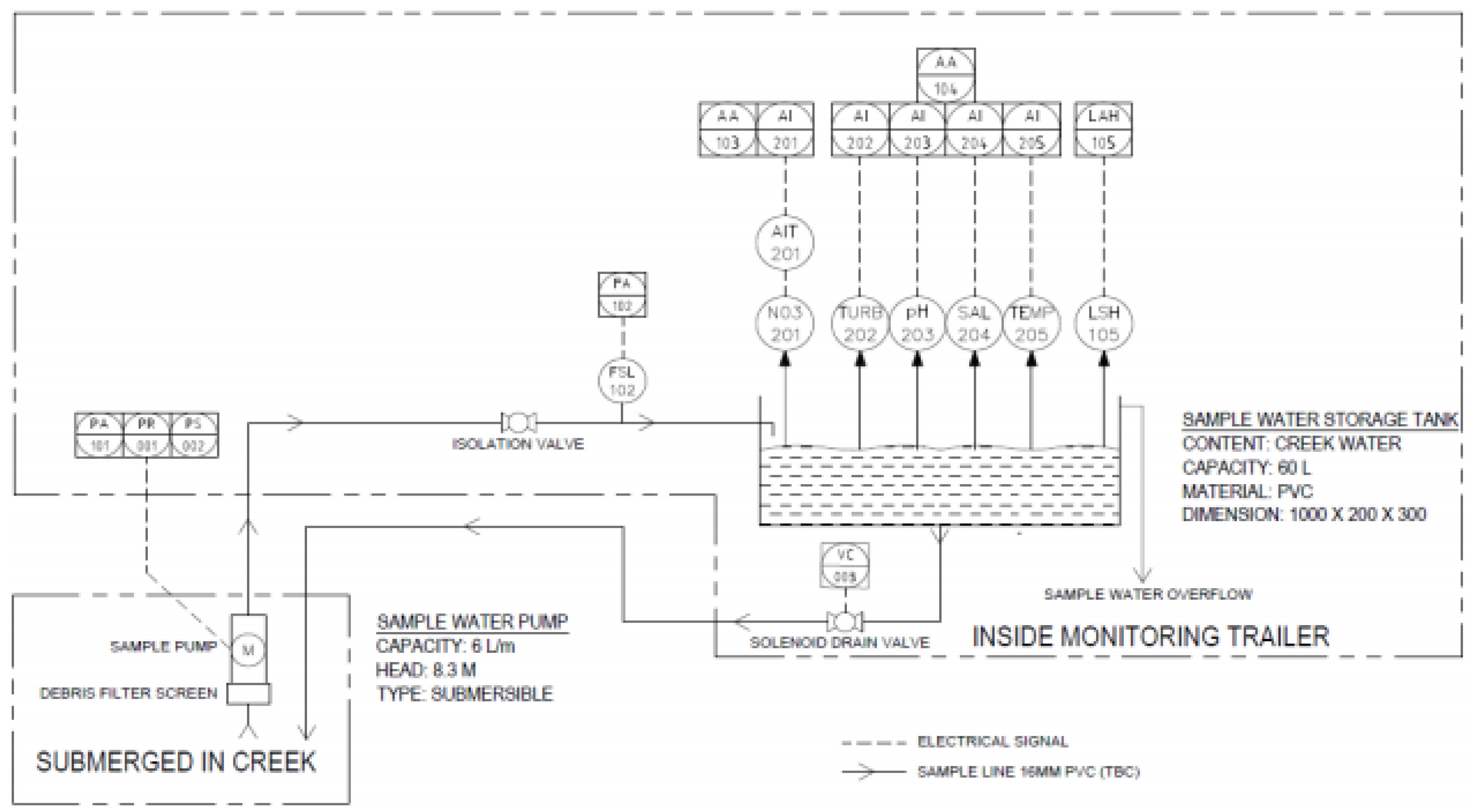
Appendix B. Piping and Instrumentation Diagram of the Mobile Trailer
A piping and instrumentation diagram is shown in
Figure A1 to reiterate the functionality of the monitoring trailer, emphasising how the design was developed to obtain water quality data.
Figure A1.
Piping and instrumentation diagram of the monitoring trailer’s functionality.
Figure A1.
Piping and instrumentation diagram of the monitoring trailer’s functionality.
Appendix C. Map of the Study Site in Ormiston, QLD
Figure A2.
Preliminary field site location at Hilliards Creek, Ormiston [
34].
Figure A2.
Preliminary field site location at Hilliards Creek, Ormiston [
34].
Appendix D. Additional Figures Comparing the NiCaVis 705 IQ to a Spectrophotometer under Different Interference Conditions
Generally, the data shown in this section highlights the efficacy of the NiCaVis 705 IQ sensor and indicates that it is much more consistent in the results it provides under a range of conditions when compared with the spectrophotometer results. Overall, the spectrophotometer was unable to accurately identify nitrates whose concentrations exceed 5 mg/L due to a saturated absorbance and the production of nitrites. For the NiCaVis 705 IQ sensor, the accuracy dropped after 25 mg/L due to the Inner Filter Effect (IFE) causing the signal to decrease.
Figure A3.
Comparison between the expected results and the spectral/sensor data under standard conditions.
Figure A3.
Comparison between the expected results and the spectral/sensor data under standard conditions.
Figure A4.
Comparison between the expected results and the spectral/sensor data with 10 mg L−1 of bromide added.
Figure A4.
Comparison between the expected results and the spectral/sensor data with 10 mg L−1 of bromide added.
Figure A5.
Comparison between the expected results and the spectral/sensor data with 20 mg L−1 of bromide added.
Figure A5.
Comparison between the expected results and the spectral/sensor data with 20 mg L−1 of bromide added.
Figure A6.
Comparison between the expected results and the spectral/sensor data with 5 µL per 50 mL potassium chloride (58,670 µs cm−1) salinity added to the samples.
Figure A6.
Comparison between the expected results and the spectral/sensor data with 5 µL per 50 mL potassium chloride (58,670 µs cm−1) salinity added to the samples.
Figure A7.
Comparison between the expected results and the spectral/sensor data with 10 µL per 50 mL potassium chloride (58,670 µs cm−1) salinity added to the samples.
Figure A7.
Comparison between the expected results and the spectral/sensor data with 10 µL per 50 mL potassium chloride (58,670 µs cm−1) salinity added to the samples.
Figure A8.
Comparison between the expected results and the spectral/sensor data with samples at pH 4.5.
Figure A8.
Comparison between the expected results and the spectral/sensor data with samples at pH 4.5.
Figure A9.
Comparison between the expected results and the spectral/sensor data with samples at pH 10.
Figure A9.
Comparison between the expected results and the spectral/sensor data with samples at pH 10.
Figure A10.
Comparison between the expected results and the spectral/sensor data with samples at 4.3 °C.
Figure A10.
Comparison between the expected results and the spectral/sensor data with samples at 4.3 °C.
Figure A11.
Comparison between the expected results and the spectral/sensor data with samples between 35–45 °C.
Figure A11.
Comparison between the expected results and the spectral/sensor data with samples between 35–45 °C.
Figure A12.
Comparison between the expected results and the spectral/sensor data with 1 NTU turbidity added.
Figure A12.
Comparison between the expected results and the spectral/sensor data with 1 NTU turbidity added.
Figure A13.
Comparison between the expected results and the spectral/sensor data with 2 NTU turbidity added.
Figure A13.
Comparison between the expected results and the spectral/sensor data with 2 NTU turbidity added.
Figure A14.
Comparison between the expected results and the spectral/sensor data with 5 NTU turbidity added.
Figure A14.
Comparison between the expected results and the spectral/sensor data with 5 NTU turbidity added.
Figure A15.
Comparison between the expected results and the spectral/sensor data with 10 NTU turbidity added.
Figure A15.
Comparison between the expected results and the spectral/sensor data with 10 NTU turbidity added.
Figure A16.
Comparison between the expected results and the spectral/sensor data with 50 NTU turbidity added.
Figure A16.
Comparison between the expected results and the spectral/sensor data with 50 NTU turbidity added.
Figure A17.
Comparison between the expected results and the spectral/sensor data with 100 NTU turbidity added.
Figure A17.
Comparison between the expected results and the spectral/sensor data with 100 NTU turbidity added.
Figure A18.
Comparison between the expected results and the spectral/sensor data with 10 mg L−1 of humic acid added.
Figure A18.
Comparison between the expected results and the spectral/sensor data with 10 mg L−1 of humic acid added.
Figure A19.
Comparison between the expected results and the spectral/sensor data with 20 mg L−1 of humic acid added.
Figure A19.
Comparison between the expected results and the spectral/sensor data with 20 mg L−1 of humic acid added.
Appendix E. Eagle.IO Online Interface
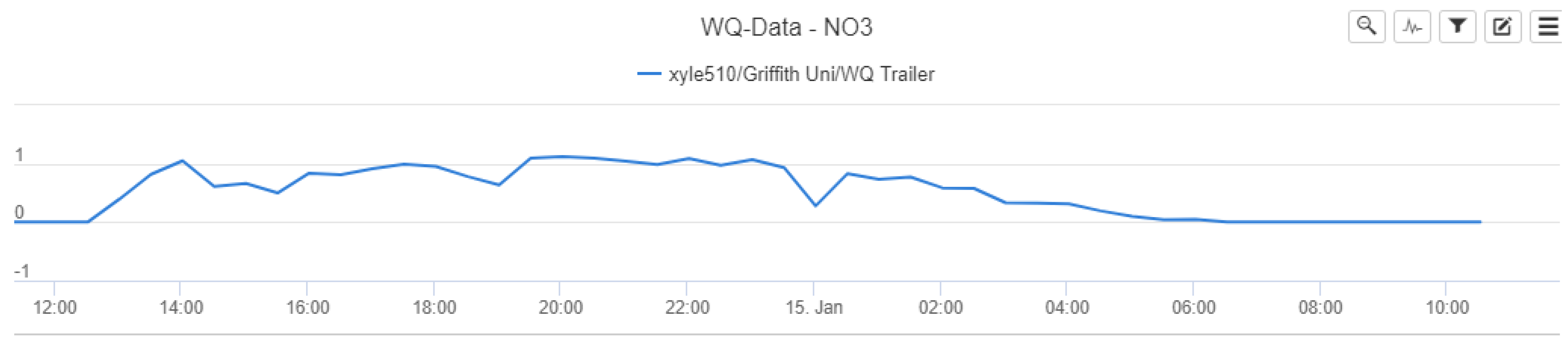
Figure A20 illustrates the online Eagle.IO interface, which was used to view data trends and identify any potential errors with the system’s operation.
Figure A20.
Eagle.IO online interface.
Figure A20.
Eagle.IO online interface.
The interface provides the data on a fixed scale, with
Figure A20 highlighting initial nitrate concentration trends on a −1 to 1 scale. From a data analysis perspective, the Eagle.IO interface was not useful in assisting to identify how consistent the reporting and results were. The data were downloaded in a.csv format for further and more detailed analyses.
References
- Omarova, A.; Tussopova, K.; Hjorth, P.; Kalishev, M.; Dosmagambetova, R. Water Supply Challenges in Rural Areas: A Case Study from Central Kazakhstan. Int. J. Environ. Res. Public Health 2019, 16, 688. [Google Scholar] [CrossRef] [PubMed]
- Matiatos, I. Nitrate source identification in groundwater of multiple land-use areas by combining isotopes and multivariate statistical analysis: A case study of Asopos basin (Central Greece). Sci. Total Environ. 2016, 541, 802–814. [Google Scholar] [CrossRef]
- Mamun, K.A.; Islam, F.R.; Haque, R.; Khan, M.G.M.; Prasad, A.N.; Haqva, H.; Mudliar, R.R.; Mani, F.S. Smart Water Quality Monitoring System Design and KPIs Analysis: Case Sites of Fiji Surface Water. Sustainability 2019, 11, 7110. [Google Scholar] [CrossRef]
- Parvez Mahmud, M.A.; Ejeian, F.; Azadi, S.; Myers, M.; Pejcic, B.; Abbassi, R.; Razmjou, A.; Asadnia, M. Recent progress in sensing nitrate, nitrite, phosphate, and ammonium in aquatic environment. Chemosphere 2020, 259, 127492. [Google Scholar] [CrossRef]
- Christensen, V.G.; Rasmussen, P.P.; Ziegler, A.C. Real-time water quality monitoring and regression analysis to estimate nutrient and bacteria concentrations in Kansas streams. Water Sci. Technol. 2002, 45, 205–219. [Google Scholar] [CrossRef] [PubMed]
- Kim, G.; Lee, Y.-W.; Joung, D.-J.; Kim, K.-R.; Kim, K. Real-time monitoring of nutrient concentrations and red-tide outbreaks in the southern sea of Korea. Geophys. Res. Lett. 2006, 33. [Google Scholar] [CrossRef]
- EcoLAB 2. Available online: https://www.labtech.com.mx/files/ecolab_2.pdf (accessed on 23 May 2020).
- Pellerin, B.A.; Stauffer, B.A.; Young, D.A.; Sullivan, D.J.; Bricker, S.B.; Walbridge, M.R.; Clyde, G.A.; Shaw, D.M. Emerging Tools for Continuous Nutrient Monitoring Networks: Sensors Advancing Science and Water Resources Protection. JAWRA 2016, 52, 993–1008. [Google Scholar] [CrossRef]
- de Oliveira, G.F.; Bertone, E.; Stewart, R.A.; Awad, J.; Holland, A.; O’Halloran, K.; Bird, S. Multi-Parameter Compensation Method for Accurate In Situ Fluorescent Dissolved Organic Matter Monitoring and Properties Characterization. Water 2018, 10, 1146. [Google Scholar] [CrossRef]
- WTW Carbovis Sensor. Available online: https://www.xylem-analytics.in/media/pdfs/wtw-carbon-carbovis-brochure.pdf (accessed on 18 May 2020).
- What Makes a River? Available online: https://www.americanrivers.org/rivers/discover-your-river/river-anatomy/ (accessed on 19 May 2020).
- Lindeburg, K.S.; Drohan, P.J. Geochemical and mineralogical characteristics of loess along northern Appalachian, USA major river systems appear driven by differences in meltwater source lithology. Catena 2019, 172, 461–468. [Google Scholar] [CrossRef]
- United States Geological Survey. Nutrients in the Nation’s Waters: Identifying Problems and Progress. Available online: https://pubs.usgs.gov/fs/fs218-96/ (accessed on 20 June 2020).
- Ayers, R.S.; Westcot, D.W. Water Quality for Agriculture. FAO Irrig. Drain. 1989, 29. [Google Scholar]
- Nitrates in Groundwater Beneath Horticultural Properties. Available online: https://www.agric.wa.gov.au/water-management/nitrates-groundwater-beneath-horticultural-properties (accessed on 19 May 2020).
- Hansen, B.; Thorling, L.; Schullehner, J.; Termansen, M.; Dalgaard, T. Groundwater nitrate response to sustainable nitrogen management. Sci. Rep. 2017, 7, 8566. [Google Scholar] [CrossRef] [PubMed]
- McLay, C.D.A.; Dragten, R.; Sparling, G.; Selvarajah, N. Predicting groundwater nitrate concentrations in a region of mixed agricultural land use: A comparison of three approaches. Environ. Pollut. 2001, 115, 191–204. [Google Scholar] [CrossRef]
- Neill, M. Nitrate concentrations in river waters in the south-east of Ireland and their relationship with agricultural practice. Water Resour. 1989, 23, 1339–1355. [Google Scholar] [CrossRef]
- Jiao, L.Z.; Dong, D.M.; Zheng, W.G.; Wu, W.B.; Feng, H.K.; Shen, C.J.; Yan, H. Determination of Nitrite Using UV Absorption Spectra Based on Multiple Linear Regression. Asian J. Chem. 2013, 25, 2273–2277. [Google Scholar] [CrossRef]
- Inagaki, T.; Watanabe, T.; Tsuchikawa, S. The effect of path length, light intensity and co-added time on the detection limit associated with NIR spectroscopy of potassium hydrogen phthalate in aqueous solution. PLoS ONE 2017, 12, e0176920. [Google Scholar] [CrossRef]
- Vidal Salgado, L.E.; Vargas-Hernandez, C. Spectrophotometric Determination of the pKa, Isosbestic Point and Equation of Absorbance vs. pH for a Universal pH Indicator. Am. J. Anal. Chem. 2014, 5, 1290–1301. [Google Scholar] [CrossRef]
- Kim, B.Y.; Yun, J.-I. Temperature effect on fluorescence and UV–vis absorption spectroscopic properties of Dy(III) in molten LiCl–KCl eutectic salt. J. Lumin. 2012, 132, 3066–3071. [Google Scholar] [CrossRef]
- Panigrahi, S.K.; Mishra, A.K. Inner filter effect in fluorescence spectroscopy: As a problem and as a solution. J. Photochem. Photobiol. C Photochem. Rev. 2019, 41, 100318. [Google Scholar] [CrossRef]
- Balali, S.; Hoseini, S.A.; Ghorbani, R.; Kordi, H. Relationships between Nutrients and Chlorophyll a Concentration in the International Alma Gol Wetland. Iran. J. Aquac. Res. Dev. 2013, 4, 173. [Google Scholar] [CrossRef]
- World Economic Outlook Database. Available online: https://www.imf.org/external/pubs/ft/weo/2019/02/weodata/index.aspx (accessed on 21 May 2020).
- Ackefors, H.; Enell, M. The release of nutrients and organic matter from aquaculture systems in Nordic countries. J. Appl. Ichthyol. 1994, 10, 225–241. [Google Scholar] [CrossRef]
- Wang, X.; Olsen, L.M.; Reitan, K.I.; Olsen, Y. Discharge of nutrient wastes from salmon farms: Environmental effects, and potential for integrated multi-trophic aquaculture. Aquac. Environ. Interact. 2012, 2, 267–283. [Google Scholar] [CrossRef]
- Marine Park Authority. Great Barrier Reef Water Quality: Current Issues. 2001. Available online: http://elibrary.gbrmpa.gov.au/jspui/bitstream/11017/358/1/GBR-water-quality-current-issues.pdf (accessed on 20 June 2020).
- Coral Bleaching and the Great Barrier Reef. Available online: https://www.coralcoe.org.au/for-managers/coral-bleaching-and-the-great-barrier-reef (accessed on 20 June 2020).
- Determining the Amount of Nitrate in Water. Available online: https://www.westminster.edu/about/community/sim/documents/SDeterminingtheAmountofNitrateinWater.pdf (accessed on 18 May 2020).
- Sterling, I. The Beginner’s Guide to Aquarium Test Strips. Available online: https://fishlab.com/aquarium-test-strips/ (accessed on 18 May 2020).
- Nitrates. Water: Monitoring and Assessment. Available online: https://archive.epa.gov/water/archive/web/html/vms57.html (accessed on 18 May 2020).
- HRWC. Nitrate: Its Importance in Water and Its Measurement. 2015. Available online: https://www.hrwc.org/wp-content/uploads/2015/03/Nitrates3-2015.pdf (accessed on 18 May 2020).
- Queensland Globe. Available online: https://qldglobe.information.qld.gov.au/ (accessed on 19 May 2020).
© 2020 by the authors. Licensee MDPI, Basel, Switzerland. This article is an open access article distributed under the terms and conditions of the Creative Commons Attribution (CC BY) license (http://creativecommons.org/licenses/by/4.0/).


