Exploring the Spatial-Temporal Relationship between Rainfall and Traffic Flow: A Case Study of Brisbane, Australia

Abstract
1. Introduction
2. Literature Review
3. Study Region and Data
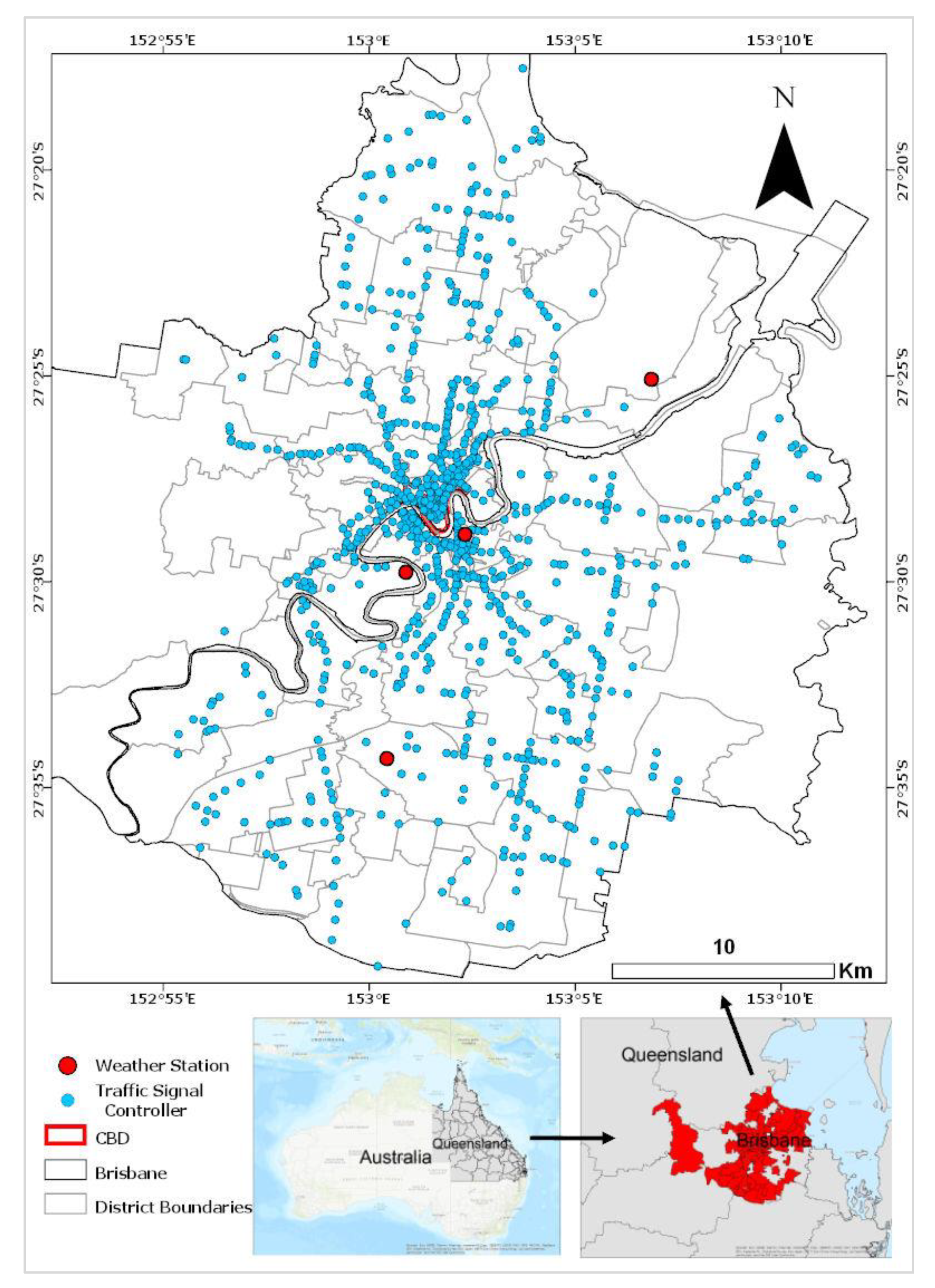
3.1. Study Region
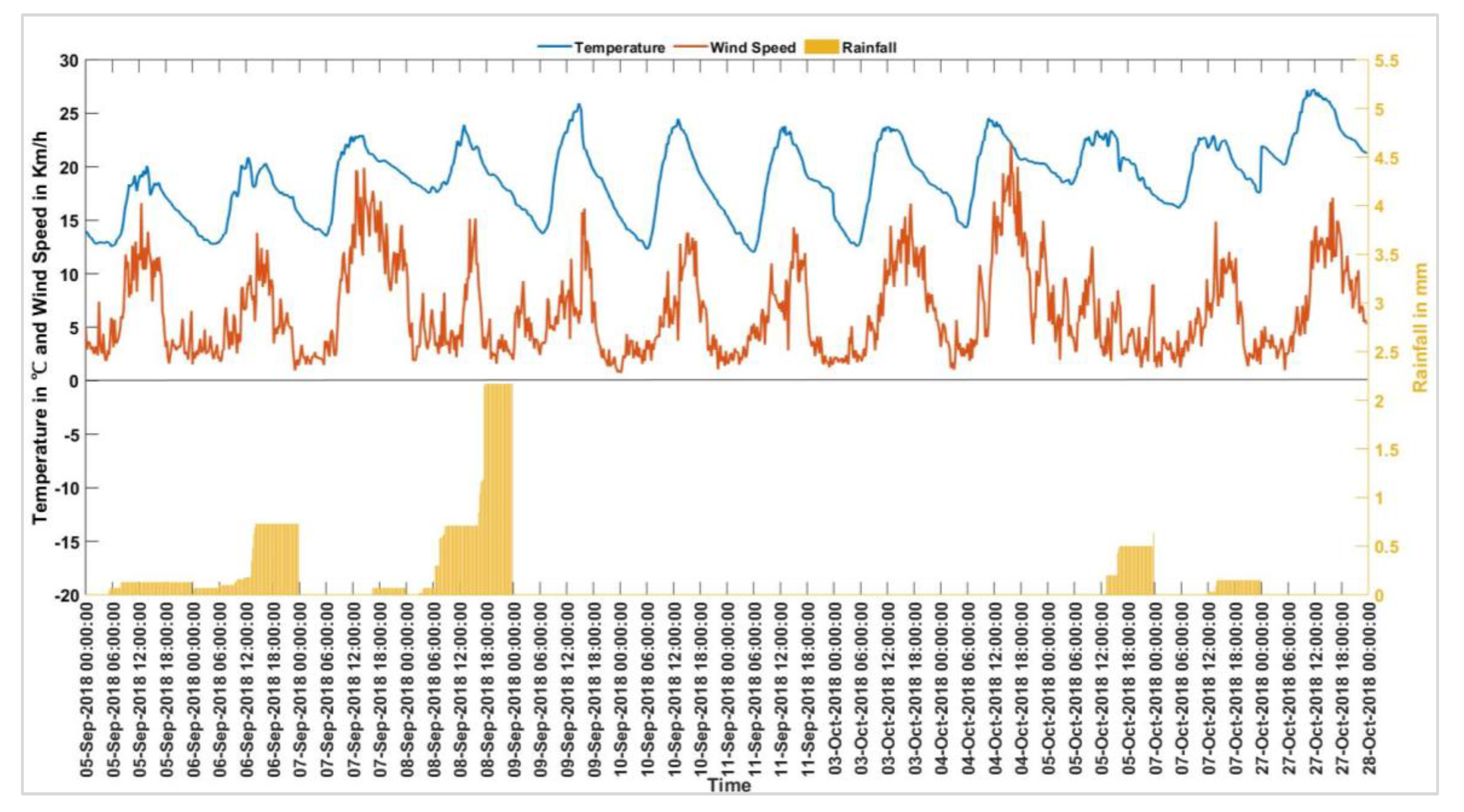
3.2. Data Collection
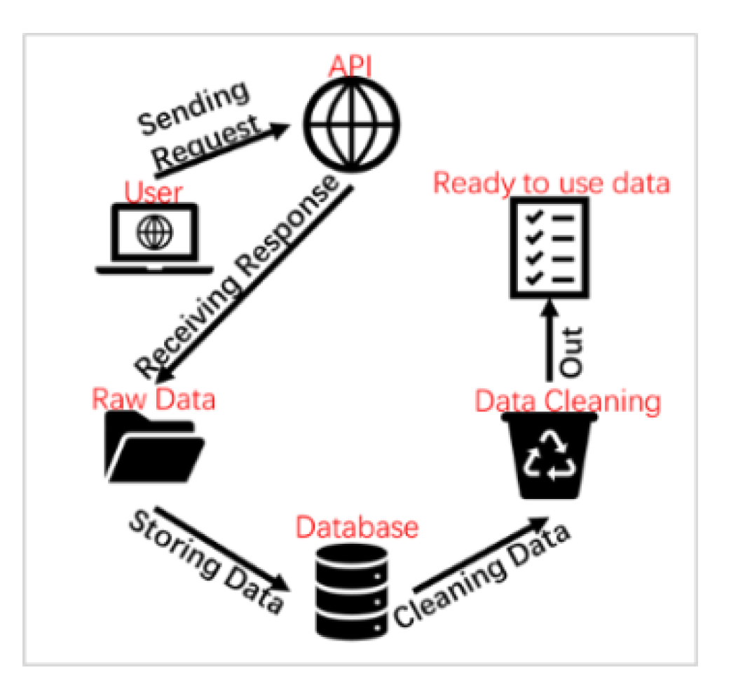
3.3. Data Sources
4. Methodology
4.1. Traffic Pattern Visualisation
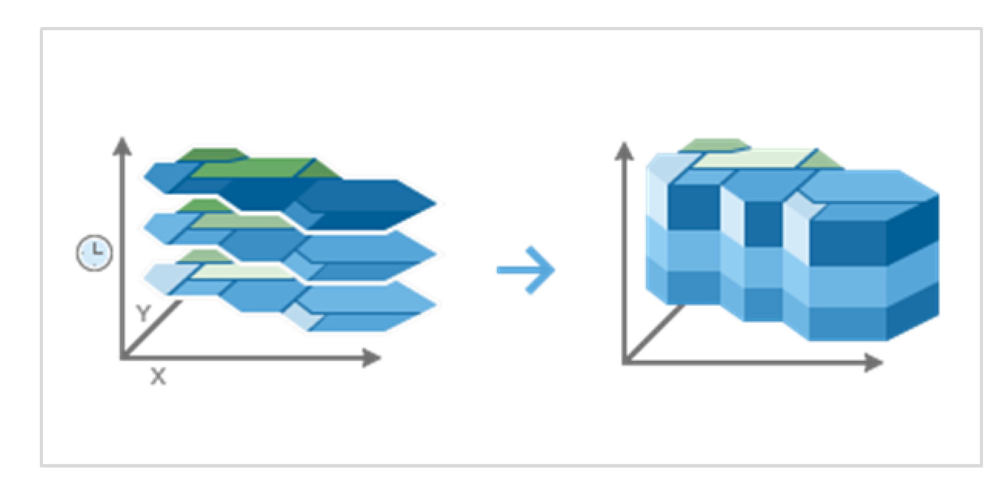
- Space-Time Cube
- Time-Series Clustering
4.2. Statistical Models
- Linear Regression (LR) Model
- Multiple Logistic Regression (MLR) Model
- Ordered Logistic Regression (OLR) Model
- Confusion Matrix
5. Results
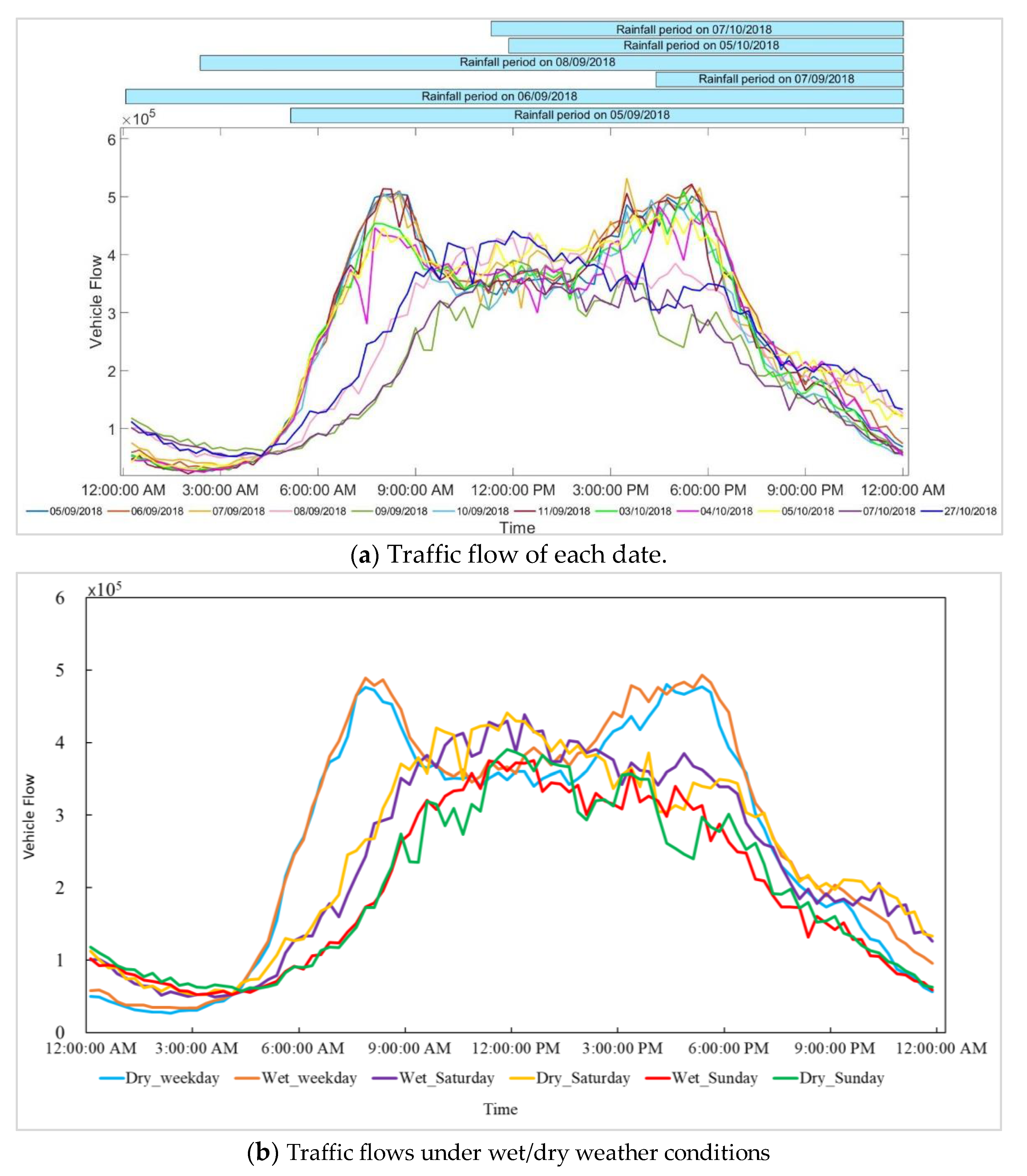
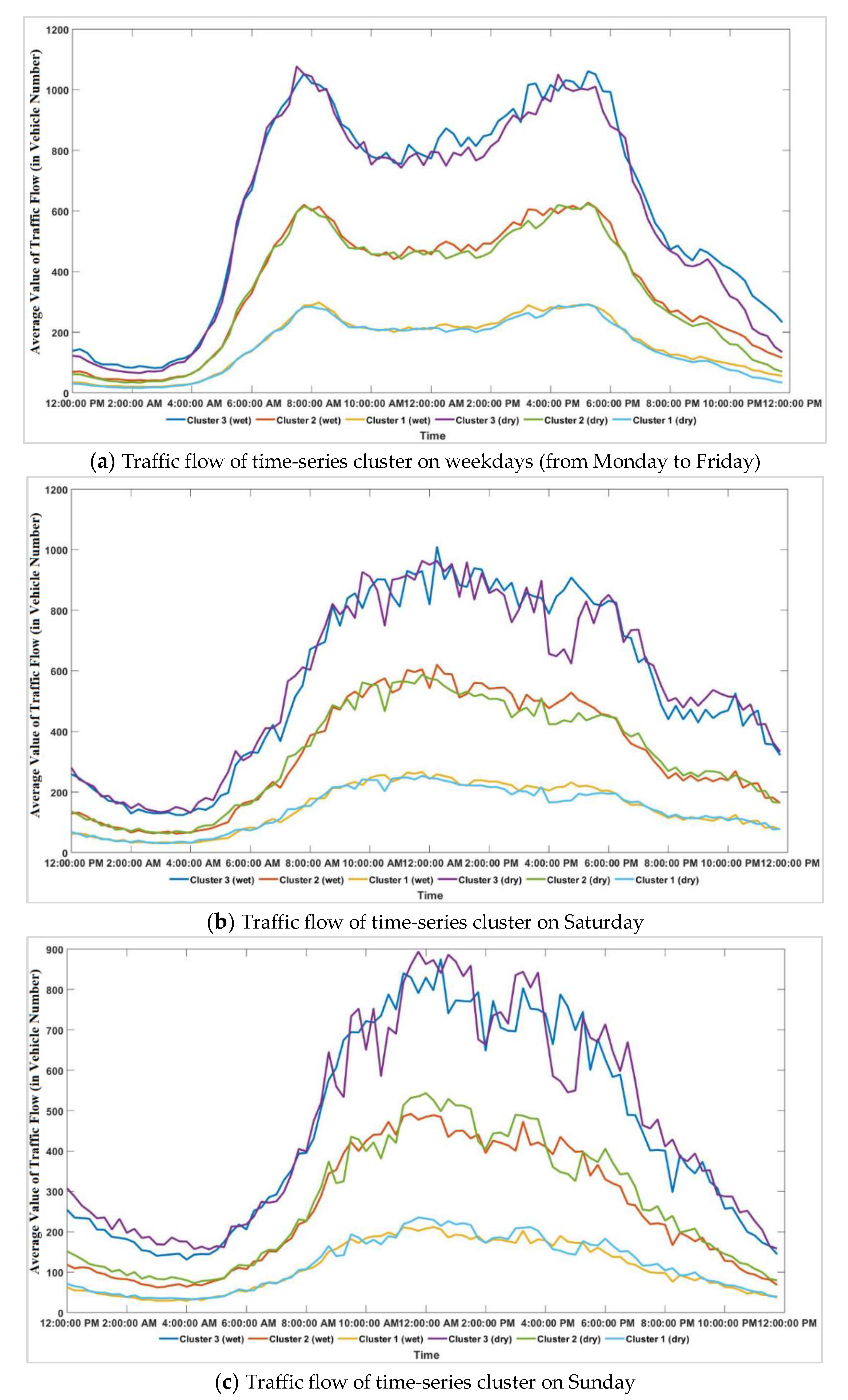
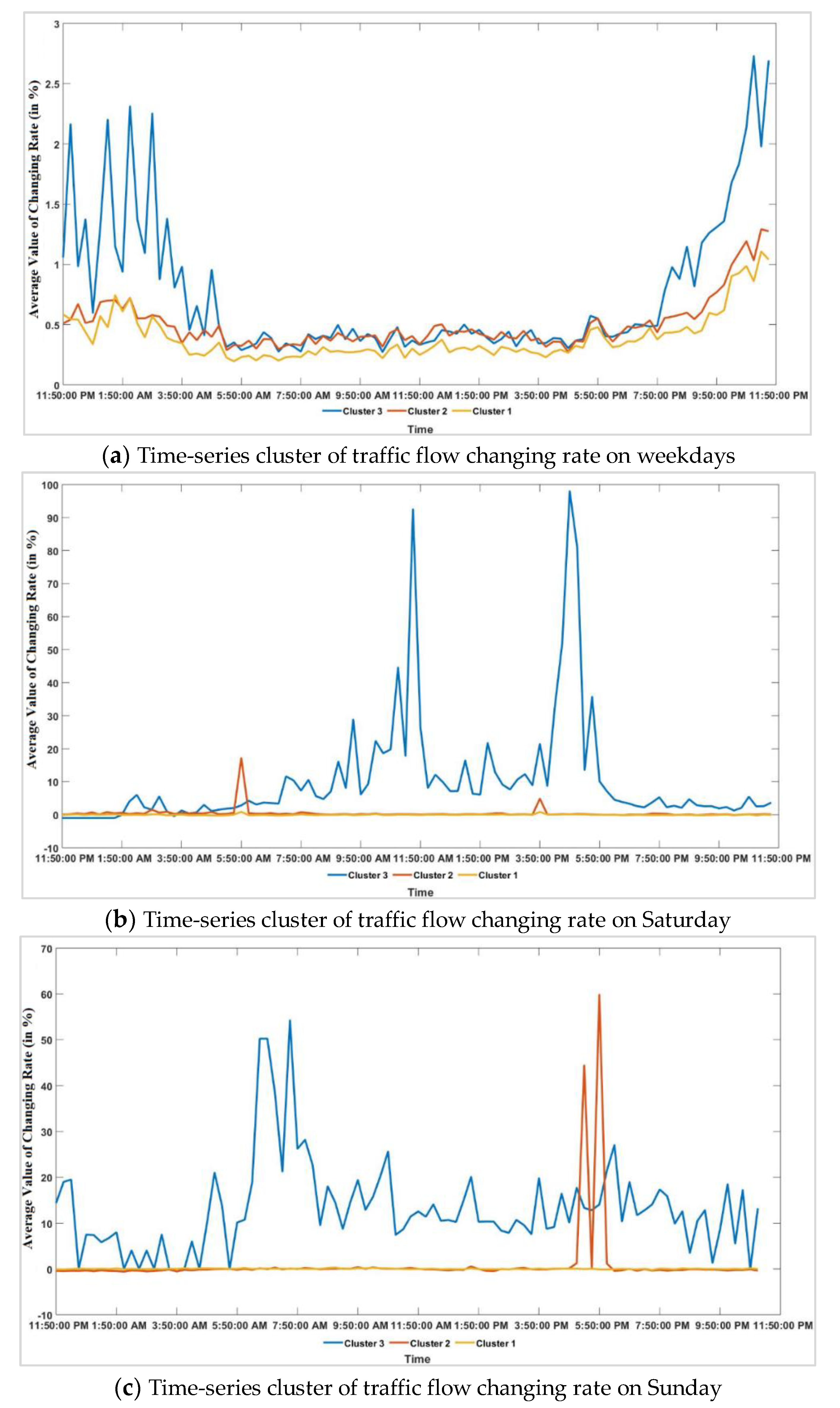
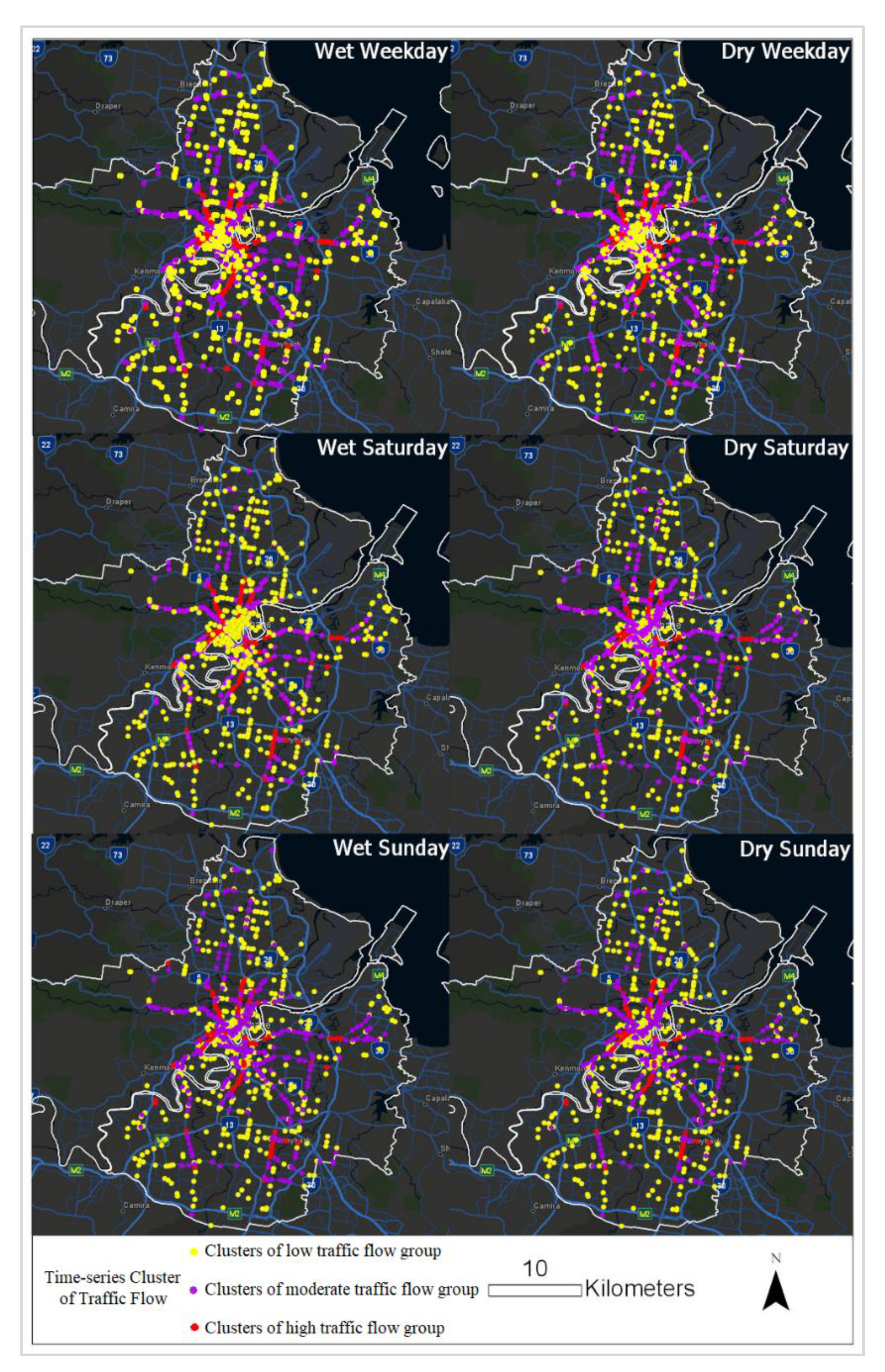
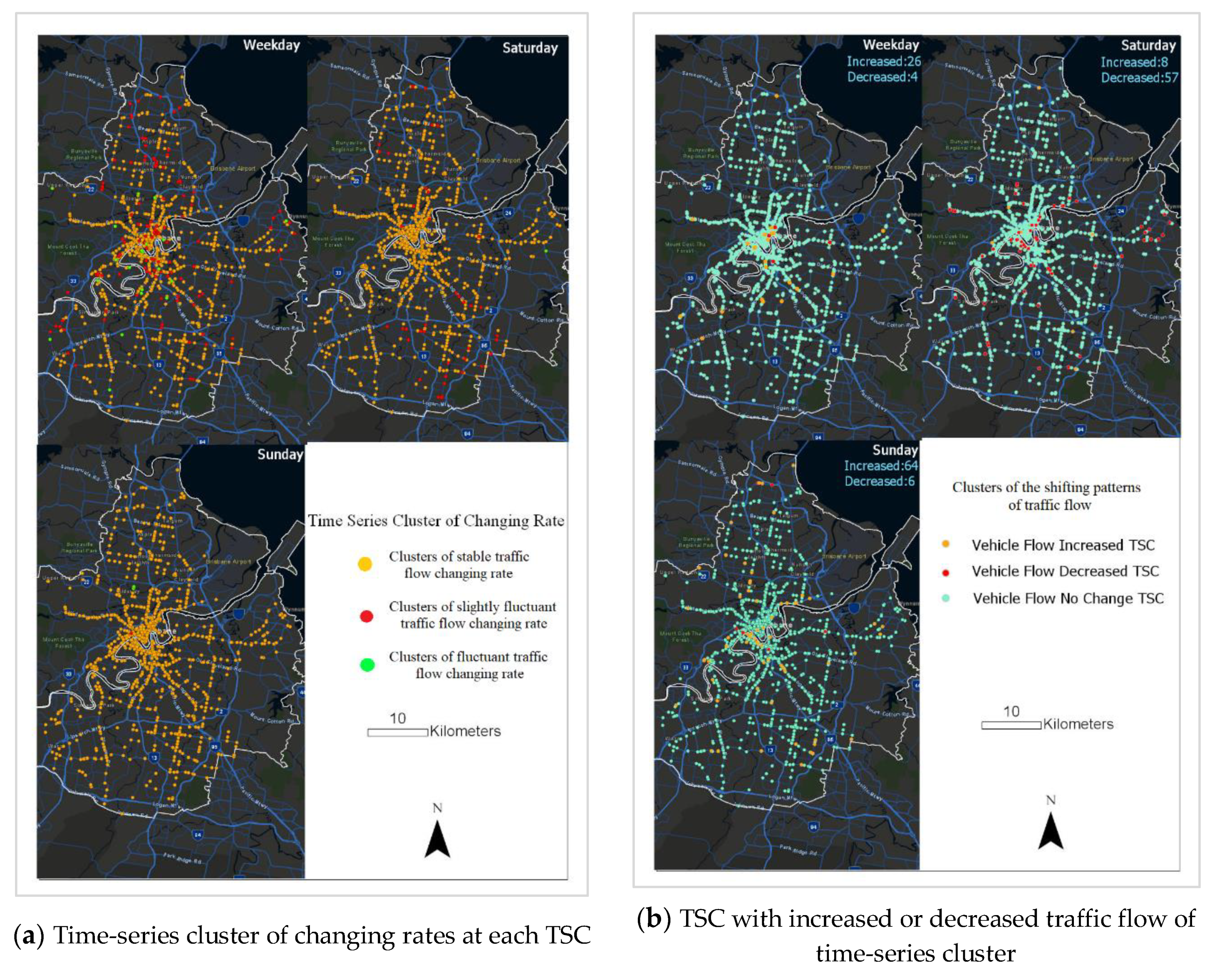
5.1. Visualisation of Traffic Flow Pattern
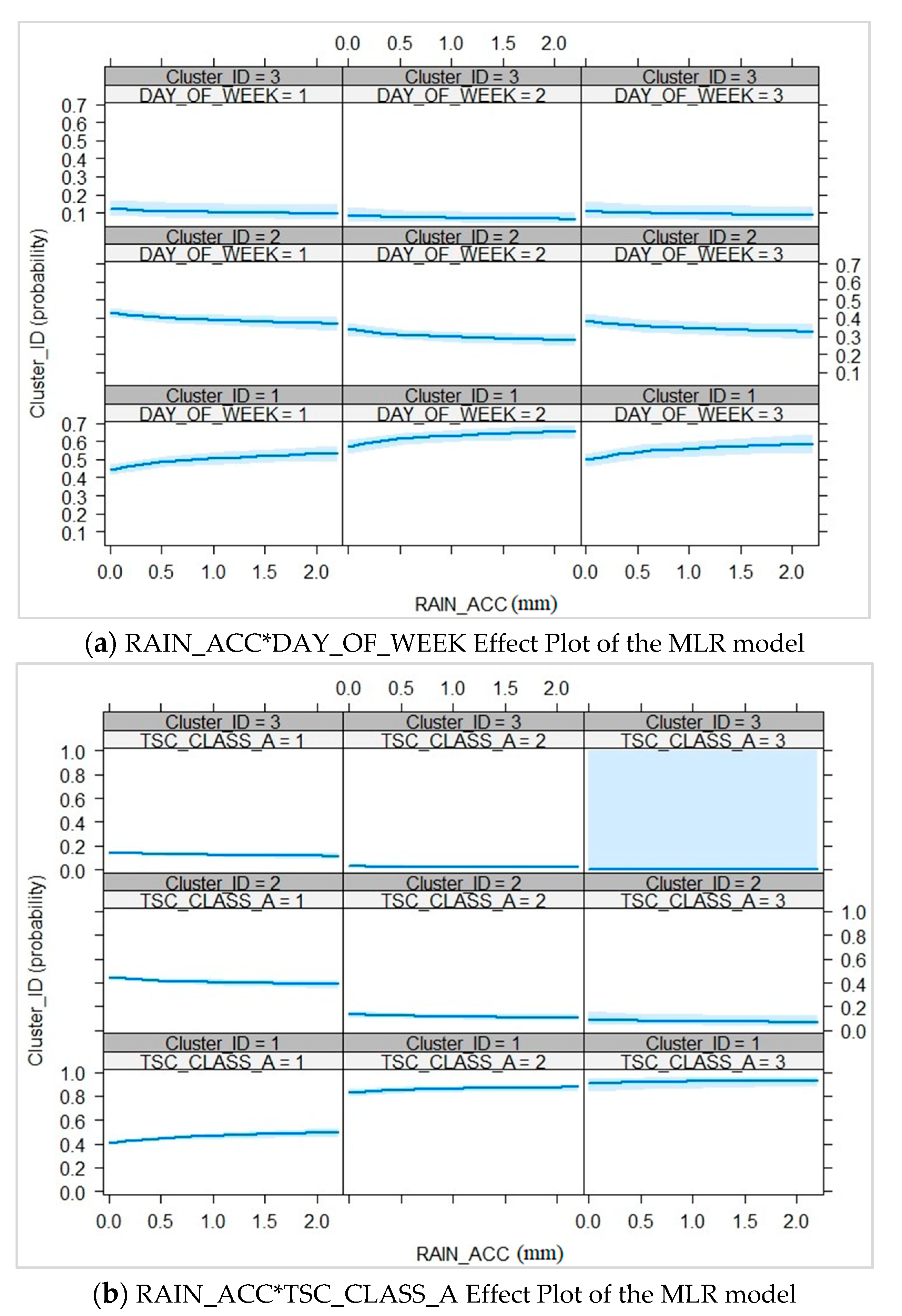
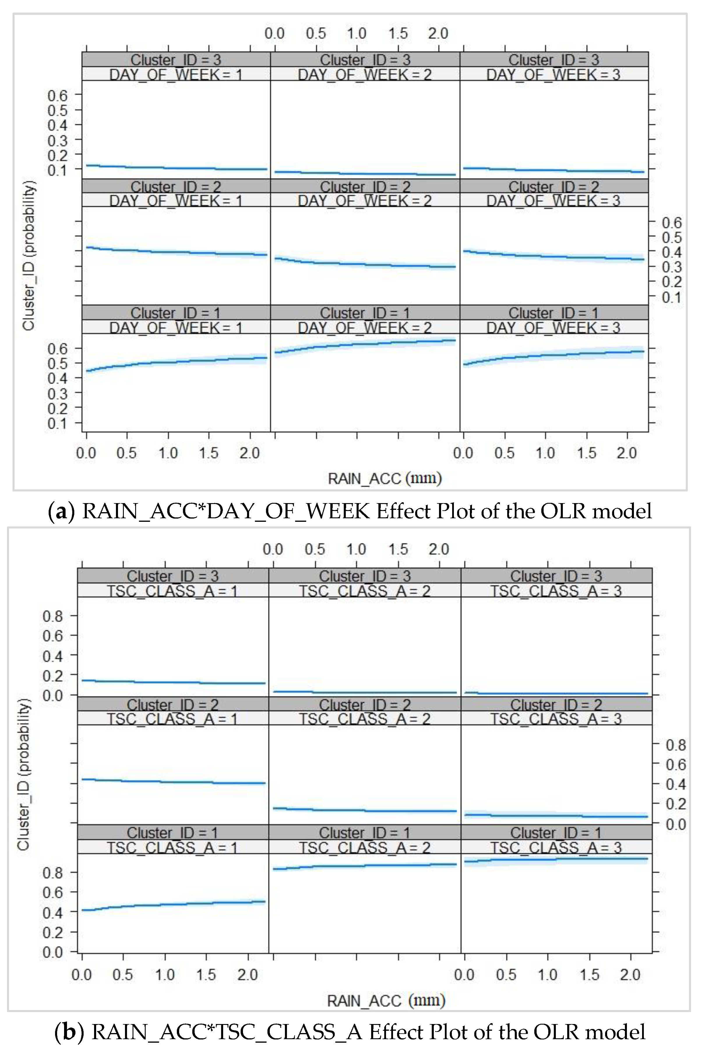
5.2. Modelling Weather’s Impact on Traffic Flow
5.2.1. Comprehensive Level
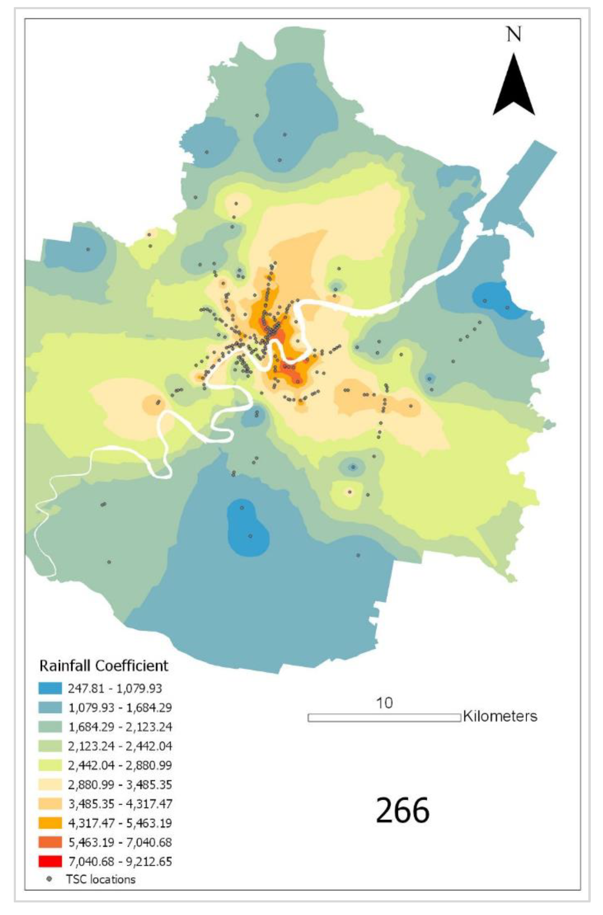
5.2.2. Location-Specific Level
5.2.3. Aggregate Level
6. Discussion and Conclusions
Author Contributions
Funding
Conflicts of Interest
References
- Li, X.; Lv, Z.; Hu, J.; Zhang, B.; Yin, L.; Zhong, C.; Wang, W.; Feng, S. Traffic Management and Forecasting System Based on 3D GIS. In Proceedings of the 2015 15th IEEE/ACM International Symposium on Cluster, Cloud and Grid Computing, Shenzhen, China, 4–7 May 2015; pp. 991–998. [Google Scholar]
- Toole, J.L.; Colak, S.; Sturt, B.; Alexander, L.P.; Evsukoff, A.; González, M.C. The path most traveled: Travel demand estimation using big data resources. Transp. Res. Part C Emerg. Technol. 2015, 58, 162–177. [Google Scholar] [CrossRef]
- Tang, J.; Liu, F.; Zhang, W.; Zhang, S.; Wang, Y. Exploring dynamic property of traffic flow time-series in multi-states based on complex networks: Phase space reconstruction versus visibility graph. Phys. A 2016, 450, 635–648. [Google Scholar] [CrossRef]
- Agarwal, M.; Maze, T.H.; Souleyrette, R. Impacts of Weather on Urban Freeway Traffic Flow Characteristics and Facility Capacity. In Proceedings of the 2005 Mid-Continent Transportation Research Symposium, Ames, IA, USA, 18–19 August 2005; pp. 1–14. [Google Scholar]
- Vlahogianni, E.I.; Karlaftis, M.G. Comparing traffic flow time-series under fine and adverse weather conditions using recurrence-based complexity measures. Nonlinear Dyn. 2012, 69, 1949–1963. [Google Scholar] [CrossRef]
- Smith, B.L.; Ulmer, J.M. Freeway traffic flow rate measurement: Investigation into impact of measurement time interval. J. Transp. Eng. 2003, 129, 223–229. [Google Scholar] [CrossRef]
- Camacho, F.J.; García, A.; Belda, E. Analysis of Impact of Adverse Weather on Freeway Free-Flow Speed in Spain. Transp. Res. Rec. 2010, 2169, 150–159. [Google Scholar] [CrossRef]
- Hassan, H.M.; Abdel-Aty, M.A. Predicting reduced visibility related crashes on freeways using real-time traffic flow data. J. Saf. Res. 2013, 45, 29–36. [Google Scholar] [CrossRef]
- Ding, Y.; Li, Y.; Deng, K.; Tan, H.; Yuan, M.; Ni, L.M. Detecting and Analyzing Urban Regions with High Impact of Weather Change on Transport. IEEE Trans. Big Data 2017, 3, 126–139. [Google Scholar] [CrossRef]
- Xie, K.; Ozbay, K.; Kurkcu, A.; Yang, H. Analysis of Traffic Crashes Involving Pedestrians Using Big Data: Investigation of Contributing Factors and Identification of Hotspots. Risk Anal. 2017, 37, 1459–1476. [Google Scholar] [CrossRef]
- Li, L.; Zhu, L.; Sui, D.Z. A GIS-based Bayesian approach for analyzing spatial-temporal patterns of intra-city motor vehicle crashes. J. Transp. Geogr. 2007, 15, 274–285. [Google Scholar] [CrossRef]
- Soltani, A.; Askari, S. Exploring spatial autocorrelation of traffic crashes based on severity. Injury 2017, 48, 637–647. [Google Scholar] [CrossRef]
- Song, Y.; Miller, H.J. Exploring traffic flow databases using space-time plots and data cubes. Transportation 2012, 39, 215–234. [Google Scholar] [CrossRef]
- Zhang, H.S.; Zhang, Y.; Li, Z.H.; Hu, D.C. Spatial-Temporal Traffic Data Analysis Based on Global Data Management Using MAS. IEEE Trans. Intell. Transp. Syst. 2004, 5, 267–275. [Google Scholar] [CrossRef]
- Theofilatos, A.; Yannis, G. A review of the effect of traffic and weather characteristics on road safety. Accid. Anal. Prev. 2014, 72, 244–256. [Google Scholar] [CrossRef] [PubMed]
- Maze, T.H.; Agarwal, M.; Burchett, G. Whether weather matters to traffic demand, traffic safety, and traffic operations and flow. Transp. Res. Rec. 2006, 1948, 170–176. [Google Scholar] [CrossRef]
- Prevedouros, P.D.; Chang, K. Potential effects of wet conditions on signalized intersection LOS. J. Transp. Eng. 2005, 131, 898–903. [Google Scholar] [CrossRef]
- Agbolosu-Amison, S.J.; Sadek, A.W.; El Dessouki, W. Inclement weather and traffic flow at signalized intersections - Case study from northern New England. Transp. Res. Rec. 2004, 1867, 163–171. [Google Scholar] [CrossRef]
- Keay, K.; Simmonds, I. The association of rainfall and other weather variables with road traffic volume in Melbourne, Australia. Accid. Anal. Prev. 2005, 37, 109–124. [Google Scholar] [CrossRef]
- Chung, E.; Ohtani, O.; Warita, H.; Kuwahara, M.; Morita, H. Effect of rain on travel demand and traffic accidents. In Proceedings of the 8th International IEEE Conference on Intelligent Transportation Systems, Vienna, Austria, 13–16 September 2005; pp. 1080–1083. [Google Scholar]
- Unrau, D.; Andrey, J. Driver Response to Rainfall on Urban Expressways. Transp. Res. Rec. 2006, 1980, 24–30. [Google Scholar] [CrossRef]
- Jaroszweski, D.; McNamara, T. The influence of rainfall on road accidents in urban areas: A weather radar approach. Travel Behav. Soc. 2014, 1, 15–21. [Google Scholar] [CrossRef]
- Mashros, N.; Ben-Edigbe, J.; Hassan, S.A.; Hassan, N.A.; Yunus, N.Z.M. Impact of Rainfall Condition on Traffic Flow and Speed: A Case Study in Johor and Terengganu. J. Teknol. 2014, 70, 65–69. [Google Scholar] [CrossRef][Green Version]
- Kamarianakis, Y.; Prastacos, P. Space–time modeling of traffic flow. Comput. Geosci. 2005, 31, 119–133. [Google Scholar] [CrossRef]
- Hou, T.; Mahmassani, H.S.; Alfelor, R.M.; Kim, J.; Saberi, M. Calibration of Traffic Flow Models under Adverse Weather and Application in Mesoscopic Network Simulation. Transp. Res. Rec. 2013, 2, 92–104. [Google Scholar] [CrossRef]
- Tao, S.; Corcoran, J.; Rowe, F.; Hickman, M. To travel or not to travel: ‘Weather’ is the question. Modelling the effect of local weather conditions on bus ridership. Transp. Res. Part C Emerg. Technol. 2018, 86, 147–167. [Google Scholar] [CrossRef]
- Datla, S.; Sharma, S. Impact of cold and snow on temporal and spatial variations of highway traffic flows. J. Transp. Geogr. 2008, 16, 358–372. [Google Scholar] [CrossRef]
- Brisbane. Available online: https://en.wikipedia.org/w/index.php?title=Brisbane&oldid=914372588 (accessed on 7 September 2019).
- Bureau of Infrastructure, Transport and Regional Economics (BITRE). Urban Public Transport: Updated Trends; Information Sheet 59; Department of Infrastructure and Regional Development of Australia: Canberra, Australia, 2014. Available online: https://www.bitre.gov.au/publications/2014/is_059 (accessed on 20 September 2019).
- Li, S.; Dragicevic, S.; Castro, F.A.; Sester, M.; Winter, S.; Coltekin, A.; Pettit, C.; Jiang, B.; Haworth, J.; Stein, A.; et al. Geospatial big data handling theory and methods: A review and research challenges. ISPRS J. Photogramm. 2016, 115, 119–133. [Google Scholar] [CrossRef]
- Yu, J.; Jiang, F.; Zhu, T. RTIC-C: A Big Data System for Massive Traffic Information Mining. In Proceedings of the 2013 International Conference on Cloud Computing and Big Data, Santa Clara Marriott, CA, USA, 27 June–2 July 2013; pp. 395–402. [Google Scholar]
- Traffic Management—Intersection Volume. Available online: https://www.data.brisbane.qld.gov.au/.data/dataset/traffic-data-at-intersection-api (accessed on 1 September 2018).
- Wei, M.; Liu, Y.; Sigler, T.; Liu, X.; Corcoran, J. The influence of weather conditions on adult transit ridership in the sub-tropics. Transp. Res. A Policy Pract. 2019, 125, 106–118. [Google Scholar] [CrossRef]
- City Plan 2014—Neighbourhood Plan Boundaries. Available online: https://www.data.brisbane.qld.gov.au/data/dataset/city-plan-2014-neighbourhood-plan-boundaries (accessed on 5 July 2019).
- Pipino, L.; Lee, Y.; Wang, R. Data quality assessment. Commun. ACM 2002, 45, 211–218. [Google Scholar] [CrossRef]
- Farber, S.; Fu, L. Dynamic public transit accessibility using travel time cubes: Comparing the effects of infrastructure (dis) investments over time. Comput. Environ. Urban Syst. 2017, 62, 30–40. [Google Scholar] [CrossRef]
- Space-Time Cube Creation. Image. 2019. Available online: https://pro.arcgis.com/en/pro-app/tool-reference/space-time-pattern-mining/createcubefromdefinedlocations.htm (accessed on 8 October 2019).
- Time-Series Clustering. Available online: https://pro.arcgis.com/en/pro-app/tool-reference/space-time-pattern-mining/time-series-clustering.htm (accessed on 20 October 2019).
- Alboukadel, K. K-Medoids in R: Algorithm and Practical Examples. 2019. Available online: https://www.datanovia.com/en/lessons/k-medoids-in-r-algorithm-and-practical-examples/#pam-algorithm (accessed on 21 October 2019).
- Zheng, Z.; Lee, J.; Saifuzzaman, M.; Sun, J. Exploring association between perceived importance of travel/traffic information and travel behavior in natural disasters: A case study of the 2011 Brisbane floods. Transp. Res. Part C Emerg. Technol. 2015, 51, 243–259. [Google Scholar] [CrossRef]
- Zheng, Z.; Liu, Z.; Liu, C.; Shiwakoti, N. Understanding public response to a congestion charge: A random effects ordered logit approach. Transp. Res. A Policy Pract. 2014, 70, 117–134. [Google Scholar] [CrossRef]
- Sun, J.; Zheng, Z.; Sun, J. Stability analysis methods and their applicability to car-following models in conventional and connected environments. Transp. Res. B Methodol. 2018, 109, 212–237. [Google Scholar] [CrossRef]
- Combinatorial Or. Available online: https://pro.arcgis.com/en/pro-app/tool-reference/spatial-analyst/combinatorial-or.htm (accessed on 21 October 2019).
- Speed Awareness Monitors-Drive Slow for SAM. Available online: https://www.brisbane.qld.gov.au/traffic-and-transport/roads-infrastructure-and-bikeways/current-road-and-intersection-projects/speedawareness-monitors (accessed on 5 July 2020).
- Aaheim, H.A.; Hauge, K.E. Impacts of climate change on travel habits: A national assessment based on individual choices. CICERO Rep. 2005, 7, 1–38. [Google Scholar]
- Koetse, M.L.; Rietveld, P. The impact of climate change and weather on transport: An overview of empirical findings. Transp. Res. D Transp. Environ. 2009, 14, 205–221. [Google Scholar] [CrossRef]


| Dataset | Data Description | Date | Data Source | |
|---|---|---|---|---|
| Traffic flow data | Recorded time TSC (Traffic Signal Controller) ID Traffic flow in each lane (4 lanes) | September 2018–October 2018 | Brisbane City Council: (https://www.data.brisbane.qld.gov.au/data/dataset/traffic-data-at-intersection-api) | |
| Weather data | Temperature (°C) Rainfall (mm) Wind speed (km/h) | September 2018–October 2018 | University of Queensland Weather Stations: (http://ww2.sees.uq.edu.au/uqweather/archive/AWS_archive/) | |
| Weather Situation (Wet/Dry) | Weekday/Weekend | Day | Date | |
| Wet | Weekday | Wednesday | 5 September 2018 | |
| Thursday | 6 September 2018 | |||
| Friday | 7 September 2018 | |||
| Friday | 5 October 2018 | |||
| Weekend | Saturday | 8 September 2018 | ||
| Sunday | 7 October 2018 | |||
| Dry | Weekday | Monday | 10 September 2018 | |
| Tuesday | 11 September 2018 | |||
| Wednesday | 3 October 2018 | |||
| Thursday | 4 October 2018 | |||
| Weekend | Sunday | 9 September 2018 | ||
| Saturday | 27 October 2018 | |||
| Category | Model | No. of Observation | AIC | df |
|---|---|---|---|---|
| Linear Regression model | Model_1 (with TSC_CLASS_A) | 10,406 | 22,8779.40 | 7 |
| Model_2 (with TSC_CLASS_B) | 10,406 | 22,8766.70 | 7 | |
| * Model_2 has smaller AIC value, which means Model_2 is better. | ||||
| Multiple Logistic Regression model | Model_3 (with TSC_CLASS_A) | 10,648 | 19,862.29 | 10 |
| Model_4 (with TSC_CLASS_B) | 10,648 | 20,700.38 | 12 | |
| * Model_3 has smaller AIC value, which means Model_3 is better. | ||||
| Ordered Logistic Regression model | Model_5 (with TSC_CLASS_A) | 10,648 | 19,849.88 | 7 |
| Model_6 (with TSC_CLASS_B) | 10,648 | 20,742.59 | 7 | |
| * Model_5 has smaller AIC value, which means Model_5 is better. | ||||
| Model | Variable | Min | Max | Mean/% | SD |
|---|---|---|---|---|---|
| Model_2 (n = 10,406) | TOTAL_FLOW | 629 | 89,188 | 26,404 | 14,635.37 |
| DAY_OF_WEEK (Weekday = 1; Saturday = 2; Sunday = 3) | 1 | 3 | Weekday = 67.12% Saturday = 16.32% Sunday = 16.57% | ||
| TSC_CLASS_B (Increased = 1; Decreased = 2; No change = 3) | 1 | 3 | Increased = 3.48% Decreased = 1.69% No change = 94.83% | ||
| RAIN_ACC (mm) | 0.00 | 2.17 | 0.32 | 0.60 | |
| Model_3/Model_5 (n = 10,648) | Cluster_ID (Low traffic flow = 1; Moderate traffic flow = 2; High traffic flow =3) | 1 | 3 | Low traffic flow = 47.36% Moderate traffic flow = 40.24% High traffic flow =12.40% | |
| TSC_CLASS_A (Stable = 1; Slightly Fluctuant = 2; Fluctuant = 3) | 1 | 3 | Stable = 88.39% Slightly Fluctuant = 10.07% Fluctuant = 1.54% | ||
| DAY_OF_WEEK (Weekday = 1; Saturday = 2; Sunday = 3) | 1 | 3 | Weekday = 66.94% Saturday = 15.97% Sunday = 17.08% | ||
| RAIN_ACC (mm) | 0.00 | 2.17 | 0.31 | 0.59 |
| Model | Variable | VIF |
|---|---|---|
| Model_2 | DAY_OF_WEEK | 1.23 |
| TSC_CLASS_B | 1.05 | |
| RAIN_ACC | 1.17 | |
| Model_3/Model_5 | DAY_OF_WEEK | 1.39 |
| TSC_CLASS_A | 2.30 | |
| RAIN_ACC | 1.42 |
| Overall Goodness-of-Fit Log Likelihood = −11,4376.4; Significance Level < 0.01; AIC = 22,8766.7 | ||||
|---|---|---|---|---|
| Variable | Estimated Value | Standard Error | t_value | Pr |
| Intercept | 26,349.5 | 785.7 | 33.537 | <0.001 |
| RAIN_ACC | 861 | 339.9 | 2.533 | 0.0113 |
| DAY_OF_WEEK = 2 | −3193.7 | 420.7 | −7.592 | <0.001 |
| DAY_OF_WEEK = 3 | −7149.6 | 392.4 | −18.221 | <0.001 |
| TSC_CLASS_B = 2 | 5767.1 | 1345.1 | 4.287 | <0.001 |
| TSC_CLASS_B = 3 | 1443.6 | 780.2 | 1.850 | 0.0643 |
| Overall Goodness-of-Fit Log Likelihood = −6910.3; Significance Level < 0.01; AIC = 19,862.29 | ||||
|---|---|---|---|---|
| Variable | Estimated Value | Standard Error | t_value | Pr |
| 1: Intercept | −0.210 | 0.038 | −5.486 | <0.001 |
| 3: Intercept | −1.111 | 0.054 | −20.751 | <0.001 |
| 1: RAIN_ACC | 0.235 | 0.063 | 3.758 | <0.001 |
| 3: RAIN_ACC | −0.064 | 0.098 | −0.656 | 0.512 |
| 1: DAY_OF_WEEK = 2 | 0.495 | 0.077 | 6.466 | <0.001 |
| 3: DAY_OF_WEEK = 2 | −0.098 | 0.121 | −0.811 | 0.417 |
| 1: DAY_OF_WEEK = 3 | 0.224 | 0.070 | 3.201 | 0.001 |
| 3: DAY_OF_WEEK = 3 | 0.027 | 0.099 | 0.268 | 0.789 |
| 1: TSC_CLASS_A = 2 | 1.868 | 0.108 | 17.257 | <0.001 |
| 3: TSC_CLASS_A = 2 | −0.432 | 0.234 | −1.849 | 0.064 |
| 1: TSC_CLASS_A = 3 | 2.349 | 0.306 | 7.676 | <0.001 |
| 3: TSC_CLASS_A = 3 | −16.447 | 1889.594 | −0.009 | 0.993 |
| Overall Goodness-of-Fit Log Likelihood = −6915.155; Significance Level < 0.01; AIC = 19,849.88 | ||||
|---|---|---|---|---|
| Variable | Estimated Value | Standard Error | t_value | Pr |
| RAIN_ACC | −0.238 | 0.056 | −4.254 | <0.001 |
| DAY_OF_WEEK = 2 | −0.487 | 0.069 | −7.066 | <0.001 |
| DAY_OF_WEEK = 3 | −0.182 | 0.062 | −2.954 | 0.003 |
| TSC_CLASS_A = 2 | −1.937 | 0.100 | −19.431 | <0.001 |
| TSC_CLASS_A = 3 | −2.629 | 0.305 | −8.611 | <0.001 |
| 1|2 | −0.476 | 0.035 | −13.670 | <0.001 |
| 2|3 | 1.651 | 0.042 | 39.549 | <0.001 |
| MLR model performance (Model_3) | |||||
| Cluster_ID | Sensitivity (%) | Specificity (%) | PPV (%) | NPV (%) | Accuracy (%) |
| 1 | 46.49 | 74.64 | 60.76 | 62.29 | 60.57 |
| 2 | 72.81 | 40.69 | 46.98 | 67.46 | 56.75 |
| 3 | 0 | 100 | NaN | 87.70 | 50.00 |
| OLR model performance (Model_5) | |||||
| Cluster_ID | Sensitivity (%) | Specificity (%) | PPV (%) | NPV (%) | Accuracy (%) |
| 1 | 38.80 | 84.50 | 67.89 | 62.05 | 61.65 |
| 2 | 82.83 | 32.66 | 47.03 | 72.49 | 57.74 |
| 3 | 0 | 100 | NaN | 87.70 | 50.00 |
| Variable | Min | Max | Mean/% | SD |
|---|---|---|---|---|
| SUM_FLOW | 22,172 | 531,976 | 253,111 | 148,766.80 |
| RAIN_ACC_15min (mm) | 0.00 | 2.17 | 0.14 | 0.37 |
| DAY_OF_WEEK (Weekday = 1; Saturday = 2; Sunday = 3) | 1 | 3 | Weekday = 66.67%; Saturday = 16.67%; Sunday = 16.67% |
| Overall Goodness-of-Fit Log Likelihood = −15,322.35; Significance Level < 0.01; AIC = 30,654.7 | ||||
|---|---|---|---|---|
| Variable | Estimated Value | Standard Error | t_value | Pr |
| Intercept | 258,525 | 5622 | 45.985 | < 0.001 |
| RAIN_ACC_15min | 72,460 | 13,828 | 5.240 | <0.001 |
| DAY_OF_WEEK = 2 | −44,527 | 12,217 | −3.645 | <0.001 |
| DAY_OF_WEEK = 3 | −67,290 | 11,718 | −5.743 | <0.001 |
© 2020 by the authors. Licensee MDPI, Basel, Switzerland. This article is an open access article distributed under the terms and conditions of the Creative Commons Attribution (CC BY) license (http://creativecommons.org/licenses/by/4.0/).
Share and Cite
Qi, Y.; Zheng, Z.; Jia, D. Exploring the Spatial-Temporal Relationship between Rainfall and Traffic Flow: A Case Study of Brisbane, Australia. Sustainability 2020, 12, 5596. https://doi.org/10.3390/su12145596
Qi Y, Zheng Z, Jia D. Exploring the Spatial-Temporal Relationship between Rainfall and Traffic Flow: A Case Study of Brisbane, Australia. Sustainability. 2020; 12(14):5596. https://doi.org/10.3390/su12145596
Chicago/Turabian StyleQi, Yanmin, Zuduo Zheng, and Dongyao Jia. 2020. "Exploring the Spatial-Temporal Relationship between Rainfall and Traffic Flow: A Case Study of Brisbane, Australia" Sustainability 12, no. 14: 5596. https://doi.org/10.3390/su12145596
APA StyleQi, Y., Zheng, Z., & Jia, D. (2020). Exploring the Spatial-Temporal Relationship between Rainfall and Traffic Flow: A Case Study of Brisbane, Australia. Sustainability, 12(14), 5596. https://doi.org/10.3390/su12145596