Application of Bipartite Networks to the Study of Water Quality

Abstract

Water is a basic natural resource for life and the sustainable development of society. Methods to assess water quality in freshwater ecosystems based on environmental quality bioindicators have proven to be low cost, reliable, and can be adapted to ecosystems with well-defined structures. The objective of this paper is to propose an interdisciplinary approach for the assessment of water quality in freshwater ecosystems through bioindicators. From the presence/absence of bioindicator organisms and their sensitivity/tolerance to environmental stress, we constructed a bipartite network, G. In this direction, we propose a new method that combines two research approaches, Graph Theory and Random Matrix Theory (RMT). Through the topological properties of the graph G, we introduce a topological index, called $JP(G)$, to evaluate the water quality, and we study its properties and relationships with known indices, such as Biological Monitoring Working Party ($BMWP$) and Shannon diversity ($H^{\prime }$). Furthermore, we perform a scaling analysis of random bipartite networks with already specialized parameters for our case study. We validate our proposal for its application in the reservoir of Guájaro, Colombia. The results obtained allow us to infer that the proposed techniques are useful for the study of water quality, since they detect significant changes in the ecosystem.

1. Introduction

One of the Sustainable Development Goals of the 2030 Agenda for Sustainable Development is to ensure the availability and sustainable management of water and sanitation for all and to preserve water quality by reducing pollution [1,2]. One of the less expensive and, at the same time, most reliable tools to assess water quality of aquatic ecosystems is the use of indicator organisms (bioindicators) of environmental stress [3,4]. Furthermore, by knowing the responses of these communities to certain environmental stressors, one can determine the cause of environmental deterioration and propose management and restoration strategies [5,6,7].

Bioindicators are living organisms that are able to modify their behavior when identifying perturbations or changes in the environment. They are used to assess changes in ecosystem health and as fundamental elements in biomonitoring of environmental quality [8]. For example, macroinvertebrate communities are often used for the biomonitoring of water quality through the application of biotic indices [9,10]. Biotic indices are numerical expressions that combine a quantitative measure of species diversity with qualitative information on the ecological sensitivity of individuals or taxons in relation to a given level of pollution [11].

In 1978, Hellawell proposed values of tolerance/sensitivity to organic pollution associated with certain families of aquatic macroinvertebrates. He established that water quality is related to the presence or absence of those families through the sum of their tolerance values, without taking into account the abundance of each taxon; the final score is the so-called and usually applied Biological Monitoring Working Party ($BMWP$) index [12,13,14]. The $BMWP$ index is calculated using the sum of the tolerance values of each identified macroinvertebrate family and indicates the degree of contamination of the studied site.

Nowadays, there are several $BMWP$ indices, all based on families of aquatic macroinvertebrates, which are currently used worldwide as a biomonitoring tool to assess water quality [15,16,17]. All $BMWP$ indices assign tolerance values between 1 and 10; the higher the score, the better the water quality [18]. One methodology to assign tolerance values associated with macroinvertebrates is the Best Professional Judgment technique [19]. This criterion consists of: (i) Collecting tolerance values of benthic macroinvertebrates from different locations, (ii) performing a statistical study of tolerance values of benthic macroinvertebrate groups, of group combinations, and of tolerance metrics, and, finally, (iii) evaluating the geographical variation of tolerance values of macroinvertebrate groups in different taxonomic levels.

Water quality studies based on aquatic macroinvertebrates often use the qualitative characteristics of the $BMWP$ index and the quantitative characteristics of the $H^{\prime }$ index [3,20,21,22,23]. The $BMWP$ index does not consider the abundance of each taxon, and the Shannon diversity index does not consider the sensitivity/tolerance to environmental stress of indicator organisms. Water quality directly affects species diversity and the presence or absence of dominant taxa in aquatic ecosystems [23,24,25,26]. By integrating the qualitative and quantitative characteristics of the $BMWP$ and $H^{\prime }$ indices into a single index, can we obtain improved results when assessing water quality?

Recently, indices associated with networks and complex systems have been introduced to study the fundamental properties of ecological systems [27,28]. These indices differ in specific parameters; for example, sensitivity in the detection of the property to be studied and robustness with respect to the size of the network. In addition, some indices simply reflect the number of species associated with the ecological system, but not their interrelations. A topological index is a quantitative measure that provides qualitative and structural information of a given system; the topological index is associated with the system invariants [29,30,31,32]. In [33], a set of topological indices describing the relationships of natural systems was presented, allowing Graph Theory to help answer fundamental questions regarding the dynamics of natural systems, but also diverse phenomena in other sciences [34,35]. It is relevant to add that most of the networks corresponding to natural and social systems have a bipartite structure; see, e.g., [36,37,38] and the references therein.

Indeed, the fundamental structures of plant or animal communities can be described mathematically [39]. In this direction and in order to assess water quality, in [40], the mathematical structure, which is a bipartite network G, was associated with the presence or absence of aquatic macroinvertebrate families and their tolerance value to pollution by means of the topological index. That topological index, named $JP(G)$, is defined as

$$JP(G):=\sum _{i=1}^{N_1}{\displaystyle \frac{{\beta }_i}{\delta ({\beta }_i)}}{log}_2\left(\prod _{iRj}{\alpha }_{ij}\right).$$

(1)

In (1), ${\beta }_i$ is the tolerance value to pollution, $\delta ({\beta }_i)$ is the number of macroinvertebrate families with the same tolerance value, and ${\alpha }_{ij}$ are the abundances of macroinvertebrate families, the relationships ($iRj$) between aquatic macroinvertebrates identified at the order level, and their tolerance value.

On the other hand, the results shown in [41], derived from the analysis and characterization of random bipartite networks, allow their application to the study of the disturbances of ecological systems represented by bipartite networks. It has been demonstrated [41] that there exist universal properties of random bipartite networks that could help us understand the dynamical behavior of the systems they represent, regardless of specific details, such as the number of vertices and connections.

The objective of this work is to propose an interdisciplinary approach for water quality assessment in freshwater ecosystems through bioindicators. For this purpose, bipartite networks provide the main element for the integration of Graph Theory and Random Matrix Theory, the two approaches used in our proposal. In the first part of this work (Section 2), we describe the construction and interpretation of the bipartite network G, representing a lentic system. Then, we formalize its analysis by means of the topological index $JP(G)$, which we always contrast with the widely used $BMWP(G)$ index,

$$BMWP(G):=\sum _{i=1}^{N_1}{\beta }_i·\delta ({\beta }_i),$$

(2)

stressing the differences and advantages of the $JP(G)$ over $BMWP(G)$. Moreover, we validate the use of the $JP(G)$ index by its application to the water quality assessment of a real-world case: The Guájaro Reservoir, Colombia. In the second part of this work (Section 3), we perform a scaling analysis of random bipartite networks with parameters already specialized on the Guájaro Reservoir. We then show that by properly defining a universal curve for the average Shannon entropy of the eigenvectors of the adjacency matrices of the bipartite network G, it is possible to define water quality classes equivalent to those obtained from the topological study of Section 2.

2. Topological Analysis to Assess Water Quality

The presence or absence of macroinvertebrate families and their tolerance or sensitivity to pollution are fundamental elements in the construction of biotic indices for the assessment of water quality. In [40], this phenomenon is represented geometrically by a bipartite network G, which is defined as follows.

Definition 1.

Let $G=G(V,E)$ be a bipartite network with weights ${\alpha }_{ij}$ and vertices $V=\{{\beta }_i,A_j\}$, where ${\beta }_i$, with $i=1,2,\cdots ,N_1$, are the tolerance values to pollution of the $N_2$ taxa of macroinvertebrate $A_j$, with $j=1,2,\cdots ,N_2$; in this case, the taxonomic identification is at the order level. E is the set of edges (relations) ${\beta }_i\sim A_j$. The vertex degree of ${\beta }_i$, denoted by $\delta ({\beta }_i)$, is the number of macroinvertebrate families characterized by the tolerance value to pollution ${\beta }_i$.

The $JP(G)$ index of Equation (1) is rewritten as

$$JP(G):=\sum _{i=1}^{N_1}{\beta }_i\sum _{{\beta }_i\sim A_j}{log}_2{({\alpha }_{ij})}^{1/\delta ({\beta }_i)}.$$

(3)

The basic definitions of Graph Theory and how to compute the $JP(G)$ index are shown in Appendix A. The construction of the network G is shown in Figure 1.

The structure of aquatic macroinvertebrate communities is defined by the number of species (richness) and their diversity. The richness of such communities can often be assessed at higher taxonomic levels; for example, gender, family, and order [42]. Furthermore, the richness measures reflect the diversity of the aquatic assembly. On the other hand, the relative abundance is the proportion of a taxon regarding all the taxa contained in an ecosystem. The relative abundance determines how rare, common, or dominant a taxon is. From now on, unless otherwise indicated, the elements of the network G are defined as follows.

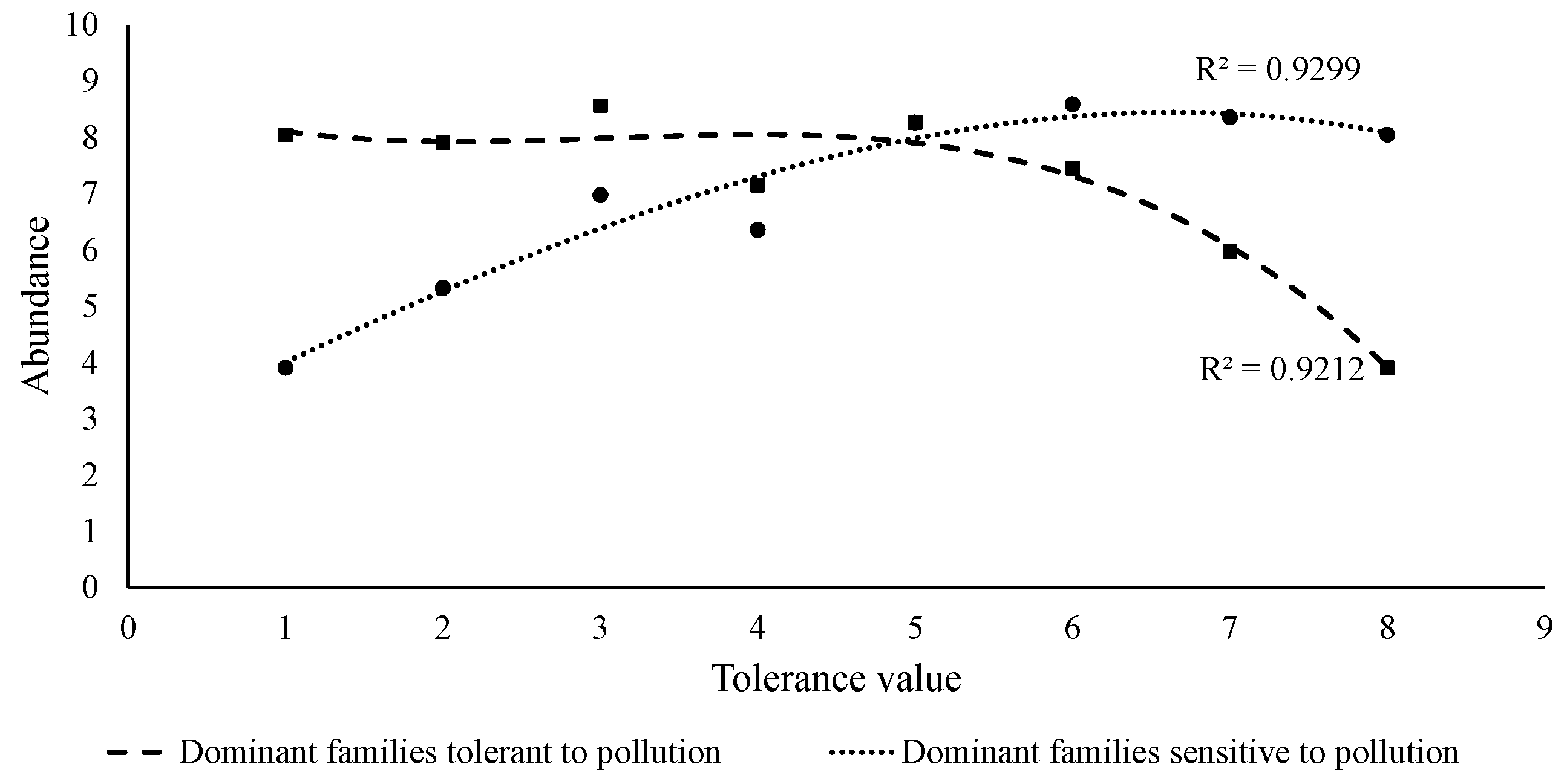
• $\nu =max\left\{{\alpha }_{ij}\right\}$ is the dominant (most abundant) taxon.
• $\phi =min\left\{{\alpha }_{ij}\right\}$ is the rare (least abundant) taxon.
• ${\mathsf{\Delta }}_i=max\left\{\delta ({\beta }_i)\right\}$ is the maximal frequency of the tolerance value ${\beta }_i$.
• ${\delta }_i=min\left\{\delta ({\beta }_i)\right\}$ is the minimum frequency of the tolerance value ${\beta }_i$.

The absence or presence of edges in network G, i.e., the absence or presence of some macroinvertebrate families, is directly related to the water quality. Thus, from the construction of the bipartite network G, we have that the fewer the number of connected components, the higher the macroinvertebrate family diversity and, thus, the better the water quality, and vice versa. The previous observation can be formalized as follows: If G contains r connected components, then there is an inverse relation between the water quality and r. As examples, in Figure 2, we show graphs with $r=1$, 3, and 8 connected components (from left to right); they describe a completely clean water system, a moderately polluted water system, and a heavily polluted water system, respectively. That is, the water quality decreases with the decrease of network connectivity $\alpha$.

The range of variation of ecological quality indices is a fundamental part of ecosystem assessment, as it allows the ecological status of the ecosystem to be classified [43]. In particular, the range of mobility of the biotic indices used for water quality assessment allows the definition of quality classes, the meaning of index ranges, and colors to make cartographic representations [12]. In this direction, Proposition A1 and (4) allow us to obtain the minimum and maximum values that the $JP(G)$ index can reach in different contexts. The next result also appears in [40]. If $N_1$ is the maximal tolerance value, then

$${log}_2(\phi )·\frac{N_1(N_1+1)}{2}\le JP(G)\le \frac{N_1(N_1+1)}{2}·{log}_2(\nu ).$$

(4)

Note that the extreme values found for the $JP(G)$ index are explicitly related to the maximal tolerance value to pollution, $N_1$ and the rare and dominant taxa. By applying the previous results to the specific problem of assessing water quality, we have that:

• If the macroinvertebrate families’ abundance in the system is uniform (${\alpha }_{ij}=k$), then $JP(G)=\frac{N_1(N_1+1)}{2}·{log}_2(\nu )$.
• The topological index $JP(G)$ is a function of the maximal abundance of one or more families, that is, it is in close relation to the load capacity of the system and the present dominant families; therefore, it provides a more objective measure than the $BMWP(G)$ index (where the presence or absence of a single family can significantly modify the water quality evaluation) and states the functional relation between the uniformity and diversity of macroinvertebrate families.

Notice that

$$\begin{array}{ccccc}JP(G)\hfill & =\hfill & {\displaystyle \sum _{i=1}^{N_1}}{\beta }_i{\displaystyle \sum _{{\beta }_i\sim A_j}}{\displaystyle \frac{1}{\delta ({\beta }_i)}}{log}_2({\alpha }_{ji})\hfill & \le \hfill & {\displaystyle \sum _{i=1}^{N_1}}{\displaystyle \frac{{\beta }_i}{\delta ({\beta }_i)}}{\displaystyle \sum _{{\beta }_i\sim A_j}}{log}_2(\nu )\hfill \\ \hfill & \le \hfill & {\displaystyle \frac{1}{{\delta }_i}}{\displaystyle \sum _{i=1}^{N_1}}{\beta }_i(\delta ({\beta }_i){log}_2(\nu ))\hfill & \le \hfill & {\displaystyle \frac{1}{{\delta }_i}}{log}_2(\nu ){\displaystyle \sum _{i=1}^{N_1}}{\beta }_i\delta ({\beta }_i)\hfill \\ \hfill & \le \hfill & {\displaystyle \frac{{log}_2(\nu )}{{\delta }_i}}BMWP(G).\hfill \end{array}$$

In addition, with a similar argument, we can get that $BMWP(G)·\frac{{log}_2(\phi )}{{\mathsf{\Delta }}_i}\le JP(G)$. Therefore, we can establish theoretical/qualitative relationships between $BMWP(G)$ and $JP(G)$ indices, and these can be formalized as follows: Given a network G, we have that

$$BMWP(G)·\frac{{log}_2(\phi )}{{\mathsf{\Delta }}_i}\le JP(G)\le BMWP(G)·\frac{{log}_2(\nu )}{{\delta }_i}.$$

On the other hand, if $N_1$ is the maximal tolerance value, then

$${\delta }_i\frac{N_1(N_1+1)}{2}\le BMWP(G)\le \frac{N_1(N_1+1)}{2}{\mathsf{\Delta }}_i.$$

(5)

Relationship (5) allows us to infer that, if all tolerance values have the same number of macroinvertebrate families, then the value of the $BMWP(G)$ index is constant (unchanged). In addition, if M is the number of macroinvertebrate families and $N_1$ is the maximal tolerance value, then

$$M\le BMWP(G)\le N_{1}M.$$

(6)

The practical implication of the Relation (6) for the study of water quality is that it allows us to know the range of the number of families of macroinvertebrates present in the experiments in relation to their tolerance values associated with the $BMWP(G)$ index. For proof of (5) and (6), see Appendix A.

Here, we define the ecological quality ratio ($EQR$), denoted by $\sigma$, as the quotient between the observed value and the expected value of the $JP(G)$ index at a reference site. As a consequence of the above results, the maximum value of the ecological status classes defined by the $JP(G)$ index will determine the $EQR$. If $N_1$ is the maximal tolerance value, then

$$\sigma =\frac{2·JP(G)}{N_1(N_1+1)·{log}_2(\nu )}.$$

(7)

Note that the value of $\sigma$ is expressed as a numerical value between 0 and 1, which implies that, if $\sigma$ approaches zero, the ecological status of the ecosystem is low, whereas if $\sigma$ approaches one, then the ecological status of the ecosystem is high. Furthermore, note that the $JP(G)$ index is normalized, so that the parameter $\sigma$ allows the stratification and evaluation of the stress level of the system as a function of the maximal tolerance value and dominant families, both measurable parameters of the system.

2.1. Water Quality Classification

Now we apply the $BMWP(G)$ and $JP(G)$ indices to a lentic system. To that end, we use the data from the sampling and tolerance values for the macroinvertebrate families identified in the Guájaro Reservoir, Colombia (for more information on the study area, see Figure 1 in [44]).

Table 1. Sampling and tolerance values for the macroinvertebrate families identified in the Guájaro Reservoir, Colombia, as reported in [44]; tolerance values ${\beta }_i$, macroinvertebrate families grouped at order level $A_j$, and  the abundance of each macroinvertebrate family ${\alpha }_{ij}$.

${\mathit{\beta }}_{\mathit{i}}$	${\mathit{A}}_{\mathit{j}}$	Family	${\mathit{\alpha }}_{\mathbf{ij}}$	${\mathit{\beta }}_{\mathit{i}}$	${\mathit{A}}_{\mathit{j}}$	Family	${\mathit{\alpha }}_{\mathbf{ij}}$
8	Trichoptera1	Xiphocentronidae	0	5	Hemiptera2	Notonectidae	55
8	Trichoptera2	Cantharidae	1	5	Hemiptera3	Naucoridae	13
8	Ephemeroptera1	Tricorythidae	0	5	Hemiptera4	Mesoveliidae	9
8	Odonata1	Gomphydae	0	5	Coleoptera5	Noteridae	288
8	Amphipoda	Gammaridae	0	5	Odonata1	Aeshnidae	2
7	Trichoptera1	Leptoceridae	39	4	Hemiptera1	Belostomatidae	109
7	Diptera1	Stratiomyidae	3	4	Diptera1	Tabanidae	33
7	Hemiptera1	Pleidae	71	4	Diptera2	Dolichopodidae	0
7	Acari	Hydrachnidae	127	4	Unionoida	Hyriidae	0
7	Hemiptera2	Corixidae	7	3	Coleoptera1	Chrysomelidae	0
7	Coleoptera1	Lampyridae	48	3	Diptera1	Tipulidae	2
7	Gastropoda1	Chilinnidae	1	3	Diptera2	Muscidae	1
6	Trichoptera	Polycentropodidae	53	3	Diptera3	Ceratopogonidae	167
6	Ephemeroptera1	Baetidae	12	3	Gastropoda1	Ampullaridae	345
6	Lepidoptera	Pyralidae	13	3	Gastropoda2	Lymnaeidae	48
6	Odonata1	Coenagrionidae	128	3	Gastropoda3	Planorbidae	383
6	Coleoptera1	Staphylinidae	3	3	Cyclostheriidae	Cyclostheriidae	0
6	Odonata2	Libellulidae	96	2	Diptera1	Culicidae	17
6	Hemiptera1	Saldidae	0	2	Hirudinidae1	Glossiphoniidae	165
6	Coleoptera2	Scirtidae	52	2	Hirudinidae2	Hirudinidae	155
6	Ephemeroptera2	Caenidae	28	2	Oligochaeta	Tubificidae	469
6	Gastropoda1	Ancylidae	112	2	Gastropoda1	Physidae	86
5	Hemiptera1	Hydrometridae	2	1	Ephemeroptera1	Polymitarcyidae	996
5	Hemiptera2	Nepidae	2	1	Gastropoda1	Hydrobiidae	6127
5	Coleoptera1	Hydrophilidae	226	1	Gastropoda2	Thiaridae	1751
5	Coleoptera2	Curculionidae	78	1	Diptera1	Chironomidae	1861
5	Coleoptera3	Dytiscidae	15	1	Diptera2	Syrphidae	14
5	Coleoptera4	Elmidae	32

is an adaptation of the data reported in Tables 3 and 6 in [44] for the Guájaro Reservoir: Macroinvertebrate families grouped at order level $A_j$, tolerance values ${\beta }_i$, and the abundance of each macroinvertebrate family ${\alpha }_{ij}$—elements used to construct the bipartite network G. The bipartite network G in Figure 3 is the geometric representation of the data in Table 1; the thickness of the edges represents the abundances of each taxon, normalized with the function ${log}_2({\alpha }_{ij}+1)$, and the macroinvertebrate family richness. We use Gephi 9.2 [45] to construct the graphs.

In general, the studies that apply the $BMWP$ index to evaluate water quality classify this quality in five classes (see [46,47] and its references). The most common approach to comparing the efficiency and scope of application of biotic indices is to compare them through their correlation with physiochemical parameters [48,49]. Here, we consider two important parameters as references: Dissolved oxygen ($DO$) and temperature (T), because there is an inverse correlation between these parameters. Changes in species composition and diversity of benthic macroinvertebrates [50,51], the $BMWP$ index [52], and water quality [53,54,55] are directly correlated with the concentration of $DO$. In particular, it has been shown that the most tolerant macroinvertebrate families to pollution are most abundant under hypoxic conditions [56], and that sensitive families to pollution are strongly associated with high concentrations of $DO$ [48]. It has been verified that values obtained for given biotic indices and the quantity of $DO$ have a direct correspondence (see, e.g., [57,58]).

To classify the water quality in our study, the class width is determined by the quotient between the expected value of the $JP(G)$ index at a reference site and the number of classes. The expected value of the $JP(G)$ index at a reference site is obtained when the average abundances are uniformly distributed and there exist all possible relations (edges) in network G (see e.g., Figure 9).

Table 2. Classification of water quality and ecological status for the Guájaro Reservoir.

Class	Water Quality	$\mathit{BMWP}(\mathit{G})$	$\mathit{DO}$ (mg/L)	$\mathit{JP}(\mathit{G})$	Stress	$\mathit{\sigma }$
I	excellent	$>231$	>9.2	>231.8	very high	0.81–1.00
II	very good	161–231	6.9–9.1	173.1–230.7	high	0.61–0.80
III	good	102–160	4.6–6.8	115.4–173.0	regular	0.41–0.60
IV	regular	46–101	2.3–4.5	57.70–115.3	low	0.21–0.40
V	low	<45	<2.2	<57.6	very low	0.00–0.20

shows the mobility ranges between classes for the $BMWP(G)$ and $JP(G)$ indices together with $DO$ for the Guájaro Reservoir. It is worth highlighting that we have an additional parameter, $\sigma$, to assess the ecological status (or stress) of the Guájaro Reservoir (see Table 2).

2.2. Comparison between Indices to Study Water Quality

On the other hand, to observe a relationship between tolerance values and abundances, each taxon was grouped according to its contamination tolerance value, and its abundances were added; the result was normalized with the logarithm function (see

Table A1. Cumulative abundances according to the tolerance values of the macroinvertebrate families shown in Table 1. Note that the abundance increases while the tolerance value decreases.

Tolerance Value	Abundance
1	10,749
2	892
3	946
4	142
5	722
6	497
7	296
8	1

).

The Shannon diversity index is one of the most important indices that frequently accompanies other indices in the assessment of water quality [24,59,60]. Its comes from information theory [61] and is applied in natural sciences to measure species diversity in biological communities. It is defined as

$$H^{\prime }=-{\displaystyle \sum _{i=1}^M}{\rho }_{i}ln({\rho }_i),$$

where ${\rho }_i$ is the relative abundance of the species i and M is the total number of species in the community. With this prescription, the larger the value of $H^{\prime }$, the larger the species diversity in a given community (and vice versa) [62,63,64]. In our application, $0\le {\rho }_i\le 50$ and $M=55$; i.e., the number of macroinvertebrate families in the Guájaro Reservoir. Finally, to support the conclusions drawn from Figure 7, we constructed 100 random samples of the macroinvertebrate families present in the Guájaro Reservoir and computed the corresponding $BMWP(G)$, $JP(G)$, and $H^{\prime }$ indices. Moreover, we computed the Pearson coefficient between these indices.

In the following section, we complete our proposal for the assessment of water quality by introducing a technique that can be used either in addition to or completely independently of the index $JP(G)$ presented above.

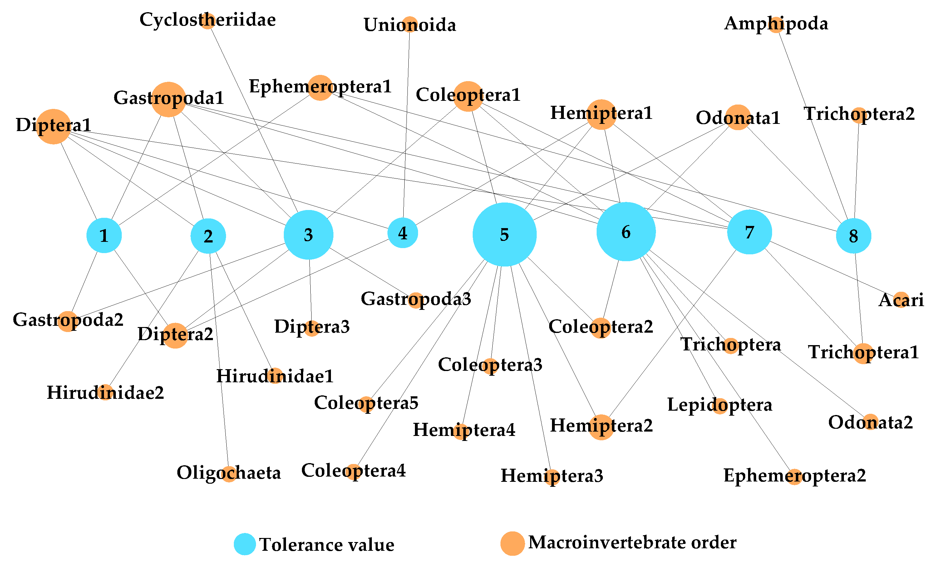
3. Spectral Analysis of the Bipartite Network $\mathit{G}$ Associated with the Guájaro Reservoir

Here, we introduce a second technique to assess water quality, which is based on the spectral properties of the bipartite network G. In particular, we will apply below the approach reported in [41], where Random Matrix Theory (RMT) was used to study the spectral properties of bipartite graphs.

Recall that network G is characterized by the sizes of the disjoint subsets, $N_1$ and $N_2$, and the connectivity $\alpha \in [0,1]$. Let $n=N_1+N_2$ and $m=min(N_1,N_2)$; i.e., n is the size of G and m the size of the smaller subset of G. We define the elements of the adjacency matrix $\mathbf{A}$ of G as

$$A_{ij}=\left\{\begin{array}{cc}\sqrt{2}{ϵ}_{ij}& \mathrm{for}i=j,\hfill \\ {ϵ}_{ij}& \mathrm{if}\mathrm{there}\mathrm{is}\mathrm{an}\mathrm{edge}\mathrm{between}\mathrm{vertices}i\mathrm{and}j,\hfill \\ 0& \mathrm{otherwise}.\hfill \end{array}\right.$$

(8)

Since we want to build an RMT ensemble, we choose ${ϵ}_{ij}$ as statistically independent random variables drawn from a normal distribution with zero mean and variance one. In addition, ${ϵ}_{ij}={ϵ}_{ji}$, since G is assumed to be undirected.

As shown in [41], a bipartite network produces block adjacency matrices when the vertices are labeled according to the subset they belong to. In Figure 4a,b, we show two examples of block adjacency matrices $\mathbf{A}$ of bipartite graphs G characterized by $n=38$ and $m=8$. Two values of $\alpha$ are used in Figure 4: 0.25 and 0.75, so that the matrix of Figure 4a is more sparse than that of Figure 4b. Note that in Figure 4, we are already using the parameter values for the network G that we are interested in: $n=38$ and $m=8$ or $N_1=8$ and $N_2=30$, as defined in the previous section.

In [41], by the scaling analysis of the average Shannon entropy $〈S〉$ of the eigenvectors of the adjacency matrices of bipartite graphs G, it was shown that the spectral and eigenvector properties of G are scaled by the parameter $\xi$. There, $\xi$ was defined as

$$\xi \equiv \frac{\alpha }{{\alpha }^{*}}$$

(9)

with

$${\alpha }^{*}=\mathcal{C}{n}^{\delta },$$

(10)

where ${\alpha }^{*}$ characterizes the localization-to-delocalization transition of the average Shannon entropy for a fixed ratio $m/n$. So, in the following, we will verify the scaling of $〈S〉$ with $\xi$ by finding the values of $\mathcal{C}$ and $\delta$ in Equation (10) for our particular application, i.e., for bipartite graphs with $n=38$ and $m=8$, and, afterwards, we will use the universal scaled curve $〈S〉$ vs. $\xi$ as a calibration curve to qualify water quality.

The Shannon entropy for the normalized eigenvector ${\mathsf{\Psi }}^k$ is given as

$$S_k=-{\displaystyle \sum _{j=1}^n}{\left|{\mathsf{\Psi }}_j^k\right|}^{2}ln{\left|{\mathsf{\Psi }}_j^k\right|}^2.$$

(11)

Indeed, in Figure 4c,d, we present $S_k$ for the eigenvectors of the adjacency matrices of panels (a,b), respectively. Note that the block structure of the adjacency matrices makes the corresponding Shannon entropies to be grouped into two sets characterized by two different average values. The groups are separated in Figure 4 by vertical dashed lines: One group corresponds to $k\in [1,8]\cup [31,38]$, and the other group to $k\in [9,30]$. However, to compute $〈S〉$ here, we average the entropies of all of the eigenvectors of the matrix $\mathbf{A}$.

Next, we use exact numerical diagonalization to compute the eigenvectors ${\mathsf{\Psi }}^k$ of the adjacency matrices of large ensembles of random bipartite graphs G characterized by the parameter set $(n,m,\alpha )$. Then, in Figure 5a, we show curves of $〈S〉$ vs. $\alpha$ for four values of the network size n for the fixed ratio $m/n=8/38$, the ratio of interest. Note that when $\alpha \to 0$, the vertices of network G are isolated and the corresponding matrix $\mathbf{A}$ is a diagonal random matrix, better known in RMT as the Poisson limit; in this case, the eigenvectors of $\mathbf{A}$ have a single component different from zero so $〈S〉=0$. In the opposite limit, $\alpha \to 1$, the bipartite network G is complete, and $〈S〉$ gets a maximum value $S_{max}$ that depends on n. Thus, to properly compare the average Shannon entropy corresponding to graphs of different sizes, we normalize it to $S_{max}$. Moreover, the curves of Figure 5a show a transition from $〈S〉\approx 0$ to $〈S〉\approx S_{max}$ as we increase $\alpha$ from $\alpha \approx 0$ to $\alpha =1$—a signature of the delocalization of the eigenvectors of $\mathbf{A}$.

It is important to stress that with the statistical study of Figure 5a, we intend to explore all possible parameter combinations of the system under study—in our case, the Guájaro Reservoir characterized by $m=8$ and $n=38$ that corresponds to the right-most curve in Figure 5a, but also of systems with equivalent characteristics; see the other curves in Figure 5a, all characterized by the ratio $m/n=8/38$.

Then, as in [41], we define the localization-to-delocalization transition point ${\alpha }^{*}$ as the value of the connectivity for which $〈S〉/S_{max}\approx 0.5$. In Figure 5b, we present ${\alpha }^{*}$ vs. n in a log–log plot where we can clearly see a power-law behavior. Therefore, the fitting of Equation (10) gives $\mathcal{C}=4.79$ and $\delta =-0.915$. Now, we are ready to verify the scaling of the Shannon entropy with the parameter $\xi$, so, in Figure 6a, we plot the curves of Figure 5a, but now as a function of $\xi$.

We can clearly see in Figure 6a that all curves $〈S〉/S_{max}$ vs. $\xi$ fall on top of the other as anticipated, since $\xi$ is the scaling parameter of the network G.

Indeed, we will use the universal curve of Figure 6a as a calibration curve to qualify water quality as follows. First, to ease the analysis in Figure 6b, we again plot the curve of Figure 6a, but interpolated, so it is now smoother. Now recall that the localized (delocalized) eigenvector regime, $〈S〉\approx 0$ ($〈S〉\approx S_{max}$), corresponds to low (high) connectivity and, accordingly, corresponds to low (high) diversity of macroinvertebrate families in our problem of water quality evaluation. Therefore, for the network G, $〈S〉\approx 0$ characterizes low water quality, while $〈S〉\approx S_{max}$ corresponds to excellent water quality. So, the eigenvector localization-to-delocalization transition depicted by the curve $〈S〉/S_{max}$ vs. $\xi$ of Figure 6b corresponds to the low-to-excellent transition in the water quality.

Therefore, we define the same five classes of water quality used in the previous section (low, regular, good, very good, and excellent) by prescribing ranges of Shannon entropy values. This prescription is quite arbitrary, so the user should choose the most appropriate one depending on the particular application. In particular, here we would like to assign the classes of low and excellent water quality to narrower ranges of $〈S〉$ than for the rest of the classes. That is, we label the water quality as low (excellent) if the Shannon entropy of the corresponding network G falls in the lower (higher) 5% window of the full range of $〈S〉$. The rest of the labels are evenly distributed in between; see Figure 6b. In

Table 3. Water quality classes according to the values of $〈S〉$, $\xi$, and $\alpha$.

Class	Water Quality	$〈\mathit{S}〉$	$\mathit{\xi }$	$\mathit{\alpha }$
I	excellent	$0.95<〈S〉\le S_{max}$	$3.888<\xi \le n$	$0.656<\alpha \le 1$
II	very good	$0.65<〈S〉\le 0.95S_{max}$	$1.300<\xi \le 3.888$	$0.219<\alpha \le 0.656$
III	good	$0.35<〈S〉\le 0.65S_{max}$	$0.774<\xi \le 1.300$	$0.131<\alpha \le 0.219$
IV	regular	$0.05<〈S〉\le S_{max}$	$0.193<\xi \le 0.774$	$0.033<\alpha \le 0.131$
V	low	$0.00<〈S〉\le 0.05S_{max}$	$0.000<\xi \le 0.193$	$0.000<\alpha \le 0.033$

, we report the Shannon entropy ranges corresponding to the five classes of water quality.

Evidently, the ranges of the Shannon entropy defining the water quality classes correspond to well-defined ranges of the parameters $\xi$ and, accordingly, $\alpha$. The ranges of $\xi$ and $\alpha$ are also reported in Table 3.

4. Result Analysis

According to (4), if we take the average abundances (259 individuals) reported in [44], we assume that all macroinvertebrate families are present, $N_1=8$, and ${log}_2(259)\approx 8$, then $JP(G)=288$ (expected value at the reference site) and $BMWP(G)=259$; thus, both indices indicate that the water quality is excellent. In this particular case, by dividing 288 by five, we get that the class width is $57.6$; see Table 2. In consequence, if there is no dominant taxon, then the $BMWP(G)$ and $JP(G)$ indices are closely related. The data reported in [44] for the Guájaro Reservoir allow the inference that $BMWP(G)=207$ and the average score by station is 166, $JP(G)=142.34$, and, on average, $DO=5.4$ mg/L, which implies that, according to the $BMWP(G)$ index, the water quality is very good, while the $DO$ and $JP(G)$ index values indicate that the water quality is just good; see Table 2. The fact that the water quality differs between the $BMWP(G)$ and $JP(G)$ indices is because the $BMWP(G)$ index does not take into account the dominant families, which, in this case, are the most tolerant to pollution ($75.26\%$); see Figure 3.

In Equation (7), if $JP(G)=142.34$, $N_1=8$, and ${log}_2(259)\approx 8$, then we have that $\sigma =0.49$. This implies that the stress level of the ecosystem is regular; see Table 2. Note that, with the application of the $JP(G)$ index and the $EQR$, we obtain similar results for water quality and ecological status.

When calculating Pearson’s correlation coefficient between the data in Table A1, we obtain that $R=-0.778(p=0.02)$; this shows that there is a negative linear correlation between tolerance values and abundances. In this direction, when we simulate samples with all the macroinvertebrate families reported in [44], but with random abundances, we observe that while the $JP(G)$ index is sensitive to population fluctuations, the value of the $BMWP(G)$ index does not change. For example, in Figure 7, we can observe significant variations of the $JP(G)$ index when there are direct or inverse correlations between abundances and tolerance values. It is important to note that when the quality of the water is low, the tendency is to find few resistant families whose abundances are high. Conversely, when water quality is good, diversity (families’ richness and abundance) should be high, including sensitive families present in lower abundances, although resistant families can be found in different types of water quality.

The calculation of Pearson’s correlation coefficient between the $BMWP(G)$, $JP(G)$, and $H^{\prime }$ indices allows us to infer that the $BMWP(G)$ and $H^{\prime }$ indices are highly correlated ($R^2=0.76$), while the correlations between the $JP(G)$ and $BMWP(G)$ indices and $JP(G)$ and $H^{\prime }$ are low ($R^2=0.07$ and $R^2=0.13$, respectively); see Figure 8. This implies that the index $JP(G)$ shows significant differences as compared to the $BMWP(G)$ and $H^{\prime }$ indices.

The scaling study of eigenvector properties of bipartite networks shown above allows us to relate the parameters $〈S〉$, $\xi$, and $\alpha$ to classes of water quality (see Table 3). To exemplify the application of the previous results on the particular case, we consider here (i.e., the Guájaro Reservoir) two cases: The hypothetical situation where all macroinvertebrate families reported in [44] are present (see Figure 9) and the actual bipartite network already shown in Figure 3. The network in Figure 9 has connectivity $\alpha =0.229$, which corresponds to a very good water quality according to Table 3, as expected, since all macroinvertebrate families are present in the lentic system. In contrast, the actual network representing the Guájaro Reservoir, shown in Figure 3, has a connectivity of $\alpha =0.191$, implying that the water quality is good; see Table 3. Note that this qualification is in complete agreement with that obtained with the application of the $JP(G)$ index in the previous section.

5. Conclusions

The geometric representation of a phenomenon associated with an ecological system allowed the study of a topological index to assess water quality. This index, the $JP(G)$ index, includes variables absent in other indices reported in the literature; for example, the qualitative and quantitative characteristics of the $BMWP$ and $H^{\prime }$ indices, dominant taxon, and macroinvertebrate family richness. In addition, the analytical properties of the network G, shown in the form of propositions, allowed us to make more objective inferences on water quality assessments because it was demonstrated that the topological index $JP(G)$ is sensitive to population dynamics, i.e., the index proposed here is capable of detecting changes in water quality from the structure of the macroinvertebrate community, changes that are not perceptible by the $BMWP$ and $H^{\prime }$ indices independently. Moreover, the ecological quality ratio $\sigma$, defined through the index $JP(G)$, describes the stress or ecological status of the ecosystem more reliably. In addition, in order to improve the definition of water quality classes, the $JP(G)$ index and the well-known $BMWP(G)$ index could also be related and compared with other indices with similar dynamics or that consider other environmental variables; for example, the Family Biotic Index or Simpson’s diversity index. This may be the subject of a future work.

The study of the spectral properties of the bipartite networks allowed us to assess water quality through the network parameters. This statistical method allows the integration of systems with a greater number of randomly related nodes, that is, it allows the integration of a greater number of macroinvertebrate families, and not only the 38 of the real-world case we consider here. This provides us with a technique that promotes the use of complex systems where non-observable relationships are present, as long as the phenomena of interest are represented by bipartite graphs.

The approach presented is associated with manual data collection. Data collection can be affected by the accessibility of sampling sites and temporality, i.e., sampling sites must be spatially well distributed, taking into account the rainy and dry seasons because, in each season, the presence of macroinvertebrates will vary and some sampling sites may not be accessible if the shape of the terrain changes. Note that the precision in the assessment of water quality may be strongly affected by the type and time of sampling, as well as the available data. For example, in our study, the data available for the Guájaro Reservoir only take into account eight levels of tolerance to pollution and 55 macroinvertebrate families; other studies report up to 10 levels of tolerance and more than 100 macroinvertebrate families, which may guarantee a better water quality assessment.

In summary, the interdisciplinary approach to water quality assessment through bioindicator organisms proposed here allowed us to associate analytical, topological, and spectral properties of bipartite graphs with water quality classes. Moreover, we stress that our approach combining Graph Theory and Random Matrix Theory techniques could be adapted and applied to other phenomena related to complex bipartite networks.

References

1. United Nations. Transforming our world: The 2030 agenda for sustainable development. In Proceedings of the General Assembley 70 Session, New York, NY, USA, 15 September 2015–13 September 2016. [Google Scholar]
2. Cantoni, J.; Kalantari, Z.; Destouni, G. Watershed-Based Evaluation of Automatic Sensor Data: Water Quality and Hydroclimatic Relationships. Sustainability 2020, 12, 396. [Google Scholar] [CrossRef] [Green Version]
3. Kumari, P.; Maiti, S.K. Bioassessment in the aquatic ecosystems of highly urbanized agglomeration in India: An application of physicochemical and macroinvertebrate-based indices. Ecol. Indic. 2020, 111, 106053. [Google Scholar] [CrossRef]
4. Dalu, T.; Chauke, R. Assessing macroinvertebrate communities in relation to environmental variables: The case of Sambandou wetlands, Vhembe Biosphere Reserve. Appl. Water Sci. 2020, 10, 16. [Google Scholar] [CrossRef] [Green Version]
5. Fan, J.; Wu, J.; Kong, W.; Zhang, Y.; Li, M.; Zhang, Y.; Meng, W. Predicting Bio-indicators of Aquatic Ecosystems Using the Support Vector Machine Model in the Taizi River, China. Sustainability 2017, 9, 892. [Google Scholar] [CrossRef] [Green Version]
6. Kattel, G.; Cai, Y.; Yang, X.; Zhang, K.; Hao, X.; Wang, R.; Dong, X. Potential Indicator Value of Subfossil Gastropods in Assessing the Ecological Health of the Middle and Lower Reaches of the Yangtze River Floodplain System (China). Geosciences 2018, 8, 222. [Google Scholar] [CrossRef] [Green Version]
7. Carvalho, R.L.; Andersen, A.N.; Anjos, D.V.; Pacheco, R.; Chagas, L.; Vasconcelos, H.L. Understanding what bioindicators are actually indicating: Linking disturbance responses to ecological traits of dung beetles and ants. Ecol. Indic. 2020, 108, 105764. [Google Scholar] [CrossRef]
8. Parmar, T.K.; Rawtani, D.; Agrawal, Y.K. Bioindicators: The natural indicator of environmental pollution. Front. Life Sci. 2016, 9, 110–118. [Google Scholar] [CrossRef] [Green Version]
9. Duran, M. Monitoring Water Quality Using Benthic Macroinvertebrates and Physicochemical Parameters of Behzat Stream in Turkey. Pol. J. Environ. Stud. 2006, 15, 5. [Google Scholar]
10. Forio, M.A.E.; Lock, K.; Radam, E.D.; Bande, M.; Asio, V.; Goethals, P.L. Assessment and analysis of ecological quality, macroinvertebrate communities and diversity in rivers of a multifunctional tropical island. Ecol. Indic. 2017, 77, 228–238. [Google Scholar] [CrossRef]
11. Czerniawska-Kusza, I. Comparing modified biological monitoring working party score system and several biological indices based on macroinvertebrates for water-quality assessment. Limnol.-Ecol. Manag. Inland Waters 2005, 35, 169–176. [Google Scholar] [CrossRef] [Green Version]
12. Alba-Tercedor, J.; Sanchez-Ortega, A. Un método rápido y simple para evaluar la calidad biológica de las aguas corrientes basado en el de Hellawell (1978). Limnetica 1988, 4, 1–56. [Google Scholar]
13. Hellawell, J.M. Biological Surveillance of Rivers: A Biological Monitoring Handbook; Water Research Centre: Stevenage, UK, 1978. [Google Scholar]
14. Hawkes, H.A. Origin and development of the biological monitoring working party score system. Water Res. 1998, 22, 964–968. [Google Scholar] [CrossRef]
15. Bieger, L.; Carvalho, A.; Strieder, M.; Maltchik, L.; Stenert, C. Are the streams of the Sinos River basin of good water quality? Aquatic macroinvertebrates may answer the question. Braz. J. Biol. 2010, 70, 1207–1215. [Google Scholar] [CrossRef] [PubMed] [Green Version]
16. Gutiérrez-Fonseca, P.E.; Ramírez, A. Evaluación de la calidad ecológica de los ríos en Puerto Rico: Principales amenazas y herramientas de evaluación. Hidrobiológica 2016, 26, 433–441. [Google Scholar]
17. Sharifinia, M.; Mahmoudifard, A.; Namin, J.I.; Ramezanpour, Z.; Yap, C.K. Pollution evaluation in the Shahrood River: Do physico-chemical and macroinvertebrate-based indices indicate same responses to anthropogenic activities? Chemosphere 2016, 159, 584–594. [Google Scholar] [CrossRef] [PubMed]
18. Armitage, P.; Moss, D.; Wright, J.; Furse, M. The performance of a new biological water quality score system based on macroinvertebrates over a wide range of unpolluted running-water sites. Water Res. 1983, 17, 333–347. [Google Scholar] [CrossRef]
19. Chang, F.-H.; Lawrence, J.E.; Rios-Touma, B.; Resh, V.H. Tolerance values of benthic macroinvertebrates for stream biomonitoring: Assessment of assumptions underlying scoring systems worldwide. Environ. Monit. Assess. 2014, 186, 2135–2149. [Google Scholar] [CrossRef]
20. Edegbene, A.O.; Elakhame, L.A.; Arimoro, F.O.; Osimen, E.C.; Odume, O.N. Development of macroinvertebrate multimetric index for ecological evaluation of a river in North Central Nigeria. Environ. Monit. Assess. 2019, 191, 274. [Google Scholar] [CrossRef]
21. Arslan, N.; Salur, A.; Kalyoncu, H.; Mercan, D.; Barişik, B.; Odabaşi, D.A. The use of BMWP and ASPT indices for evaluation of water quality according to macroinvertebrates in Küçük Menderes River (Turkey). Biologia 2016, 71, 49–57. [Google Scholar] [CrossRef]
22. Wondmagegn, T.; Mengistou, S. Effects of anthropogenic activities on macroinvertebrate assemblages in the littoral zone of Lake Hawassa, a tropical Rift Valley Lake in Ethiopia. Lakes Reserv. Res. Manag. 2020, 25, 61–71. [Google Scholar] [CrossRef]
23. Luo, K.; Hu, X.; He, Q.; Wu, Z.; Cheng, H.; Hu, Z.; Mazumder, A. Impacts of rapid urbanization on the water quality and macroinvertebrate communities of streams: A case study in Liangjiang New Area, China. Sci. Total. Environ. 2018, 621, 1601–1614. [Google Scholar] [CrossRef] [PubMed]
24. Patang, F.; Soegianto, A.; Hariyanto, S. Benthic macroinvertebrates diversity as bioindicator of water quality of some rivers in East Kalimantan, Indonesia. Int. J. Ecol. 2018, 2018, 5129421. [Google Scholar] [CrossRef]
25. Zand, S.M. Indexes associated with information theory in water quality. J. Water Pollut. Control. Fed. 1976, 48, 2026–2031. [Google Scholar]
26. Gualdoni, C.M.; Oberto, A.M. Estructura de la comunidad de macroinvertebrados del arroyo Achiras (Córdoba, Argentina): Análisis previo a la construcción de una presa. Iheringia SéRie Zool. 2012, 102, 177–186. [Google Scholar] [CrossRef] [Green Version]
27. Delmas, E.; Besson, M.; Brice, M.-H.; Burkle, L.A.; Dalla Riva, G.V.; Fortin, M.-J.; Gravel, D.; Guimarães, P.R., Jr.; Hembry, D.H.; Newman, E.A.; et al. Analysing ecological networks of species interactions. Biol. Rev. 2019, 94, 16–36. [Google Scholar] [CrossRef] [Green Version]
28. Koutrouli, M.; Karatzas, E.; Paez-Espino, D.; Pavlopoulos, G.A. A Guide to Conquer the Biological Network Era Using Graph Theory. Front. Bioeng. Biotechnol. 2020, 8, 34. [Google Scholar] [CrossRef]
29. Hernandez-Gomez, J.C.; Romero-Valencia, J.; Carreto, R.R. Mathematical Aspects on the Harmonic Index. Int. J. Math. Anal. 2017, 11, 85–95. [Google Scholar] [CrossRef]
30. Ramirez, A.; Reyna, G.; Rosario, O. Spectral study of the inverse index. Adv. Appl. Discret. Math. 2018, 19, 195–211. [Google Scholar] [CrossRef]
31. Sigarreta, J.M. Bounds for The Geometric-Arithmetic Index of a Graph. Miskolc Math. Notes 2015, 16, 1199–1212. [Google Scholar] [CrossRef] [Green Version]
32. Jordan, F.; Scheuring, I. Network ecology: Topological constraints on ecosystem dynamics. Phys. Life Rev. 2004, 1, 139–172. [Google Scholar] [CrossRef]
33. Navia, A.F.; Cortes, E.; Mejia-Falla, P.A. Topological analysis of the ecological importance of elasmobranch fishes: A food web study on the Gulf of Tortugas, Colombia. Ecol. Model. 2010, 221, 2918–2926. [Google Scholar] [CrossRef]
34. Rodriguez, A.; Infante, D. Network models in the study of metabolism. Electron. J. Biotechnol. 2009, 12, 11–12. [Google Scholar]
35. Aguilar-Becerra, C.D.; Frausto-Martínez, O.; Avilés-Pineda, H.; Pineda-Pineda, J.J.; Caroline Soares, J.; Reyes- Umaña, M. Path Dependence and Social Network Analysis on Evolutionary Dynamics of Tourism in Coastal Rural Communities. Sustainability 2019, 11, 4854. [Google Scholar] [CrossRef] [Green Version]
36. Dormann, C.F.; Fründ, J.; Blüthgen, N.; Gruber, B. Indices, graphs and null models: Analyzing bipartite ecological networks. Open Ecol. J. 2009, 2, 7–24. [Google Scholar] [CrossRef]
37. Holme, P.; Liljeros, F.; Edling, C.R.; Kim, B.J. Network bipartivity. Phys. Rev. E 2003, 68, 056107. [Google Scholar] [CrossRef] [PubMed] [Green Version]
38. Pasquaretta, C.; Jeanson, R. Division of labor as a bipartite network. Behav. Ecol. 2017, 29, 342–352. [Google Scholar] [CrossRef]
39. Hellawell, J.M. Biological Indicators of Freshwater Pollution and Environmental Management; Elsevier Science Publishers Ltd.: New York, NY, USA, 2012. [Google Scholar]
40. Pineda-Pineda, J.J.; Rosas-Acevedo, J.L.; Hernandez-Gomez, J.C.; Rosario, O.; Sigarreta, J.M. Approximation to the Study of Water Quality. Appl. Math. Sci. 2018, 12, 421–430. [Google Scholar] [CrossRef]
41. Martínez-Martínez, C.T.; Méndez-Bermúdez, J.A.; Moreno, Y.; Pineda-Pineda, J.J.; Sigarreta, J.M. Spectral and localization properties of random bipartite graphs. Chaos Solitons Fractals X 2019, 3, 100021. [Google Scholar] [CrossRef]
42. Barbour, M.T.; Gerritsen, J.; Snyder, B.D.; Stribling, J.B. Rapid Bioassessment Protocols for Use in Streams and Wadeable Rivers: Periphyton, Benthic Macroinvertebrates and Fish; US Environmental Protection Agency, Office of Water: Washington, DC, USA, 1999; Volume 339.
43. Carayon, D.; Eulin-Garrigue, A.; Vigouroux, R.; Delmas, F. A new multimetric index for the evaluation of water ecological quality of French Guiana streams based on benthic diatoms. Ecol. Indic. 2020, 113, 106248. [Google Scholar] [CrossRef]
44. Romero, K.C.; Del Rio, J.P.; Villarreal, K.C.; Anillo, J.C.C.; Zarate, Z.P.; Gutierrez, L.C.; Franco, O.L.; Valencia, J.W.A. Lentic water quality characterization using macroinvertebrates as bioindicators: An adapted BMWP index. Ecol. Indic. 2017, 72, 53–66. [Google Scholar] [CrossRef]
45. Bastian, M.; Heymann, S.; Jacomy, M. Gephi: An open source software for exploring and manipulating networks. ICWSM 2009, 8, 361–362. [Google Scholar]
46. Ministerio del Ambiente y Energia; Ministra de Salud. Reglamento para la Evaluación y Clasificación de la Calidad de Cuerpos de Agua Superficiales No. 33903-MINAE-S. Available online: http://www.digeca.go.cr/sites/default/files/de-33903reglamento_evaluacion_clasificacion_cuerpos_de_agua_0.pdf (accessed on 8 June 2020).
47. Pineda-Pineda, J.J.; Rosas-Acevedo, J.L.; Sigarreta, J.M.; Hernández-Gómez, J.C.; Reyes-Umaña, M. Biotic Indices to Evaluate Water Quality: BMWP. Int. J. Environ. Ecol. Fam. Urban Stud. (IJEEFUS) 2018, 8, 23–36. [Google Scholar]
48. Everaert, G.; De Neve, J.; Boets, P.; Dominguez-Granda, L.; Mereta, S.T.; Ambelu, A.; Thas, O. Comparison of the abiotic preferences of macroinvertebrates in tropical river basins. PLoS ONE 2014, 9, e108898. [Google Scholar] [CrossRef] [PubMed] [Green Version]
49. Yazdian, H.; Jaafarzadeh, N.; Zahraie, B. Relationship between benthic macroinvertebrate bio-indices and physicochemical parameters of water: A tool for water resources managers. J. Environ. Health Sci. Eng. 2014, 12, 30. [Google Scholar] [CrossRef] [Green Version]
50. Kaller, M.D.; Kelso, W.E. Association of macroinvertebrate assemblages with dissolved oxygen concentration and wood surface area in selected subtropical streams of the southeastern USA. Aquat. Ecol. 2007, 41, 95–110. [Google Scholar] [CrossRef]
51. Wilson, P.C. Water Quality Notes: Dissolved Oxygen. Sea 2010, 1000, 5000. [Google Scholar]
52. Hooda, P.S.; Moynagh, M.; Svoboda, I.F.; Miller, A. Macroinvertebrates as bioindicators of water pollution in streams draining dairy farming catchments. Chem. Ecol. 2000, 17, 17–30. [Google Scholar] [CrossRef]
53. Hynes, H.B.N. The Ecology of Running Waters; Liverpool University Press: Liverpool, UK, 1970; p. 555. [Google Scholar]
54. Schreier, H.; Erlebach, W.; Albright, L. Variations in water quality during winter in two Yukon rivers with emphasis on dissolved oxygen concentration. Water Res. 1980, 14, 1345–1351. [Google Scholar] [CrossRef]
55. Tixier, G.; Felten, V.; Guérold, F. Life cycle strategies of Baetis species (Ephemeroptera, Baetidae) in acidified streams and implications for recovery. Fundam. Appl. Limnol. Hydrobiol. 2009, 174, 227–243. [Google Scholar] [CrossRef]
56. Connolly, N.M.; Crossland, M.R.; Pearson, R.G. Effect of low dissolved oxygen on survival, emergence, and drift of tropical stream macroinvertebrates. J. N. Am. Benthol. Soc. 2004, 23, 251–270. [Google Scholar] [CrossRef]
57. Koçer, M.A.T.; Sevgili, H. Parameters selection for water quality index in the assessment of the environmental impacts of land-based trout farms. Ecol. Indic. 2014, 36, 672–681. [Google Scholar] [CrossRef]
58. Zamora-Muñoz, C.; Sáinz-Cantero, C.E.; Sánchez-Ortega, A.; Alba-Tercedor, J. Are biological indices BMPW’and ASPT’and their significance regarding water quality seasonally dependent? Factors explaining their variations. Water Res. 1995, 29, 285–290. [Google Scholar] [CrossRef]
59. Zhao, C.; Pan, T.; Dou, T.; Liu, J.; Liu, C.; Ge, Y.; Zhang, Y.; Yu, X.; Mitrovic, S.; Lim, R. Making global river ecosystem health assessments objective, quantitative and comparable. Sci. Total. Environ. 2019, 667, 500–510. [Google Scholar] [CrossRef] [PubMed]
60. Clairmont, L.K.; Slawson, R.M. Contrasting water quality treatments result in structural and functional changes to wetland plant-associated microbial communities in lab-scale mesocosms. Microb. Ecol. 2020, 79, 50–63. [Google Scholar] [CrossRef]
61. Shannon, C.E.; Weaver, W. The Mathematical Theory of Communication 1949; University of Illinois Press: Urbana, IL, USA, 1949. [Google Scholar]
62. Magnussen, S.; Boyle, T. Estimating sample size for inference about the Shannon-Weaver and the Simpson indices of species diversity. For. Ecol. Manag. 1995, 78, 71–84. [Google Scholar] [CrossRef]
63. Pla, L. Biodiversidad: Inferencia basada en el índice de Shannon y la riqueza. Interciencia 2006, 31, 583–590. [Google Scholar]
64. Jørgensen, S.E.; Xu, F.L.; Salas, F.; Marques, J.C. Handbook of Ecological Indicators for Assessment of Ecosystem Health; CRC Press: Boca Raton, FL, USA, 2016; pp. 9–64. [Google Scholar]
Figure 1. Scheme of the bipartite network G ( V , E ) with weights α i j and vertices V = { β i , A j } , where β i , with i = 1 , 2 , , N 1 , are the tolerance values to pollution of the N 2 taxa of macroinvertebrate A j , with j = 1 , 2 , , N 2 . In G, each edge represents a different macroinvertebrate family whose thickness depends on the relative abundance. Note that the vertices of the set A j need the taxonomic identification to be at the order level; thus, one should be careful on their labeling because different macroinvertebrate families could have the same order with different tolerance values to pollution.
Sustainability 12 05143 g001
Figure 2. Bipartite networks with 1, 3, and 8 connected components (ac) respectively.
Sustainability 12 05143 g002
Figure 3. Bipartite network G of 38 nodes ( m = 8 and n = 30 ) and 46 edges. General relations for the data are in Table 1. Note that the dominant families are most tolerant to pollution. The isolated vertices are the macroinvertebrate families with zero abundance.
Sustainability 12 05143 g003
Figure 4. Nonzero adjacency matrix elements A i j of a single realization of random bipartite graphs G with n = 38 and m = 8 . (a) α = 0.25 and (b) α = 0.75 . (c,d) The Shannon entropies S k of ten realizations of random graphs with the parameters of the corresponding upper panels.
Sustainability 12 05143 g004
Figure 5. (a) Shannon entropy S as a function of the connectivity α for random bipartite graphs G characterized by the ration m / n = 8 / 38 for four different network sizes n = 38 , 76, 152, and 304. S is normalized to S m a x . To compute each symbol in the figure, we average over 10 6 eigenvectors. (b) Localization-to-delocalization transition point α * as a function of n. The dashed line is the power-law fitting of the data with Equation (10). From the fitting, we get C = 4.79 and δ = 0.915 .
Sustainability 12 05143 g005
Figure 6. (a) Shannon entropy curves of Figure 5a as a function of ξ . (b) The universal curve S / S m a x vs. ξ . Horizontal lines indicate the regions of different water quality classes. The vertical dashed lines at ξ = 0.193 and ξ = 3.888 delimit the low and excellent water quality classes; see Table 3.
Sustainability 12 05143 g006
Figure 7. Abundance versus tolerance values for dominant families tolerant to pollution and dominant families sensitive to pollution. Here, samples of the macroinvertebrate families present in the Guájaro Reservoir were simulated. When the dominant families are tolerant to pollution, the value of the J P ( G ) index is 135. On the other hand, if the dominant families are sensitive to pollution, J P ( G ) = 176 . In both cases B M W P ( G ) = 259 .
Sustainability 12 05143 g007
Figure 8. Scatter plots between B M W P ( G ) , J P ( G ) , and Shannon diversity indices for 100 random samples of the macroinvertebrate families present in the Guájaro Reservoir. The index values are normalized with the function log 2 ( x + 1 ) .
Sustainability 12 05143 g008
Figure 9. Bipartite network of 38 nodes ( m = 8 and n = 30 ) and 55 edges associated with the Guájaro Reservoir in the hypothetical situation where all macroinvertebrate families reported in [44] are present. Here, α = 0.229 , in contrast to the actual bipartite network of Figure 3 with α = 0.191 .
Sustainability 12 05143 g009