Integrated Evaluation of Changing Water Resources in an Active Ecotourism Area: The Case of Puerto Princesa City, Palawan, Philippines

Abstract

Rapid urbanization, tourism, and climate change (CC) threaten water resource management in developing countries. Conventional water-planning tools cannot account for the changing effects of water disparity, climate risks, and environmental flow (EF) requirements. This paper proposes an alternative approach that applies stylized water-demand forecasting and predicting water availability from the perspectives of CC, changing society, and EF, thereby providing managers with future scenarios of surface water sufficiency/deficiency in an active ecotourism area, namely, Puerto Princesa City, Philippines. We considered (1) scenarios of seasonal droughts to prepare for climate risks in the future and (2) scenarios of water availability that do not depend on groundwater supply, in which the projected water deficiency is frequent both annually and seasonally. The results of this case study showed that an additional water supply from the Montible Watershed to the city was projected to secure sufficient amounts of water to achieve surface-water sufficiency, which is consistent with the goals of both the municipality and the water company to reduce the dependency on groundwater. Moreover, significant infrastructure investment costs must be anticipated in Scenario 3. Our approach proves efficient in modeling water demand in regions with active tourism and hydrology and therefore has the potential for further analyses and application.

1. Introduction

In the Anthropocene, human activities have had tremendous impacts on local environments, and these activities have now manifested as global issues such as climate change. It is essential to consider human activities and climate change in water resource management [1,2,3,4,5]. While climate change leads to changes in freshwater ecosystems, changes in human water demands cause serious water stresses that have intensified in already water-stressed regions [6,7,8].

Tourism is an important industry in low-income countries and alters the consumption pattern of water in concerned areas [9,10]. The increase in water consumption caused by tourism is often not considered in water planning. Estimates suggest that 80–3500 L of water per tourist per overnight stay is consumed [11,12,13]. Although tourism can bring high economic benefits [14,15], it has also negative impacts on the natural water environment. The overexploitation of water resources is particularly sensitive in coastal and island destinations [16,17]. Overuse of water and ignoring environmental flow (EF) requirements cause ecological degradation in many parts of the world. For example, the Australian government has reallocated water to the environment at a substantial expense to mitigate the significant degradation suffered by the Murray–Darling Basin [18]. Maintenance of EF requirements should also be viewed as a measure of sustainability in water resource management and considered in water supply planning and implementation [19]. Sociohydrological changes and their impacts on the natural environment must be comprehensively considered and evaluated to achieve sustainable development, especially in areas that mainly rely on income from tourism.

This study aims to fill the research gap by integrating climate-change-induced hydrological processes, changes in the consumption of water for domestic and commercial purposes, and the environment for sustainable surface-water development in an active site for ecotourism. We consider multiple water-demand scenarios that account for the influence of tourists, local conditions, and water supply scenarios to provide options for the sustainable exploitation of surface-water sources under the influence of climate change. We highlight the adequacy of surface water resources to provide insights on surface-water development in the study region.

2. Study Region

In the Philippines, tourism accounts for 8.6% of the country’s gross domestic product (GDP) [20]. Ecotourism plays a significant role in providing livelihood opportunities and serves as a tool for conservation in the Philippines. The study area, Puerto Princesa City (PPC) in Palawan Island (Figure 1), is one of the major ecotourism destinations in the country, where tourist arrivals and the population are increasing each year (Figure 2). Despite the sudden increase in tourist arrivals since 2009, the assumptions for planning and designing water-supply systems have remained unchanged, thereby ignoring the changing water consumption patterns.

In 2011, a 25-million-liter day⁻¹ (MLD)-capacity infiltration gallery (IG) was built upstream of the Irawan River (Figure 1) in addition to the 5 MLD IG that existed downstream. Based on the 2016 monthly report, the river supplied 43%, and 29 deep wells supplied 57% of the water requirement of the service area. Water shortage is experienced during summer, when tourist arrivals peaks and little precipitation is expected, leading to an increased reliance on groundwater supply. Saltwater intrusion has already been observed in one of the wells managed by the Puerto Princesa City Water District (PPCWD) (based on an interview with the PPCWD). This has led to a proposal to develop a new surface-water source, the Lapu–Lapu watershed, to better meet the current and future water demands.

The Puerto Princesa City (PPC) municipality encompasses a total land area of approximately 220,000 ha, 70% of which is covered by forests. The topography is mainly hilly to mountainous (65%), where only 35% of the land is close to sea level or has a gently sloping terrain. The region is influenced by a tropical monsoon climate, which is characterized by a short dry season, followed by several months of heavy rainfall. The average annual rainfall is 1553 mm. The highest and lowest recorded rainfall were 2594 mm in 1999 and 986 mm in 1991, respectively. The daily average minimum and maximum temperatures are 24.7 °C and 32.6 °C, respectively.

At present, the primary water system of the PPCWD is limited to the service area where 77% (or 196,119) of the population is concentrated and where middle-high-income groups are typically found. This is partly explained by the group’s ability to pay, which shapes the extension and improvement of the water system, and the potential demand from socioeconomic activities in the area. As of 2015, only 74% of the households in the service area were metered, and this is projected to increase as the population and income increase, and as the resilience of the water supply to adverse changes improves.

3. Data and Methods

This study involves three steps: (1) assessment and projection of water availability and water demand, (2) model calibration and evaluation, and (3) integrated scenario analyses. The hydrometeorological output of the Soil and Water Assessment Tool (SWAT v.12, developed and supplied by the United States Department of Agricultural Research Service at the Blackland Research & Extension Center in Temple, Texas, USA) was used to determine water availability [21]. Water demand was classified as domestic, commercial, institutional, and tourism based on population and tourist arrivals. 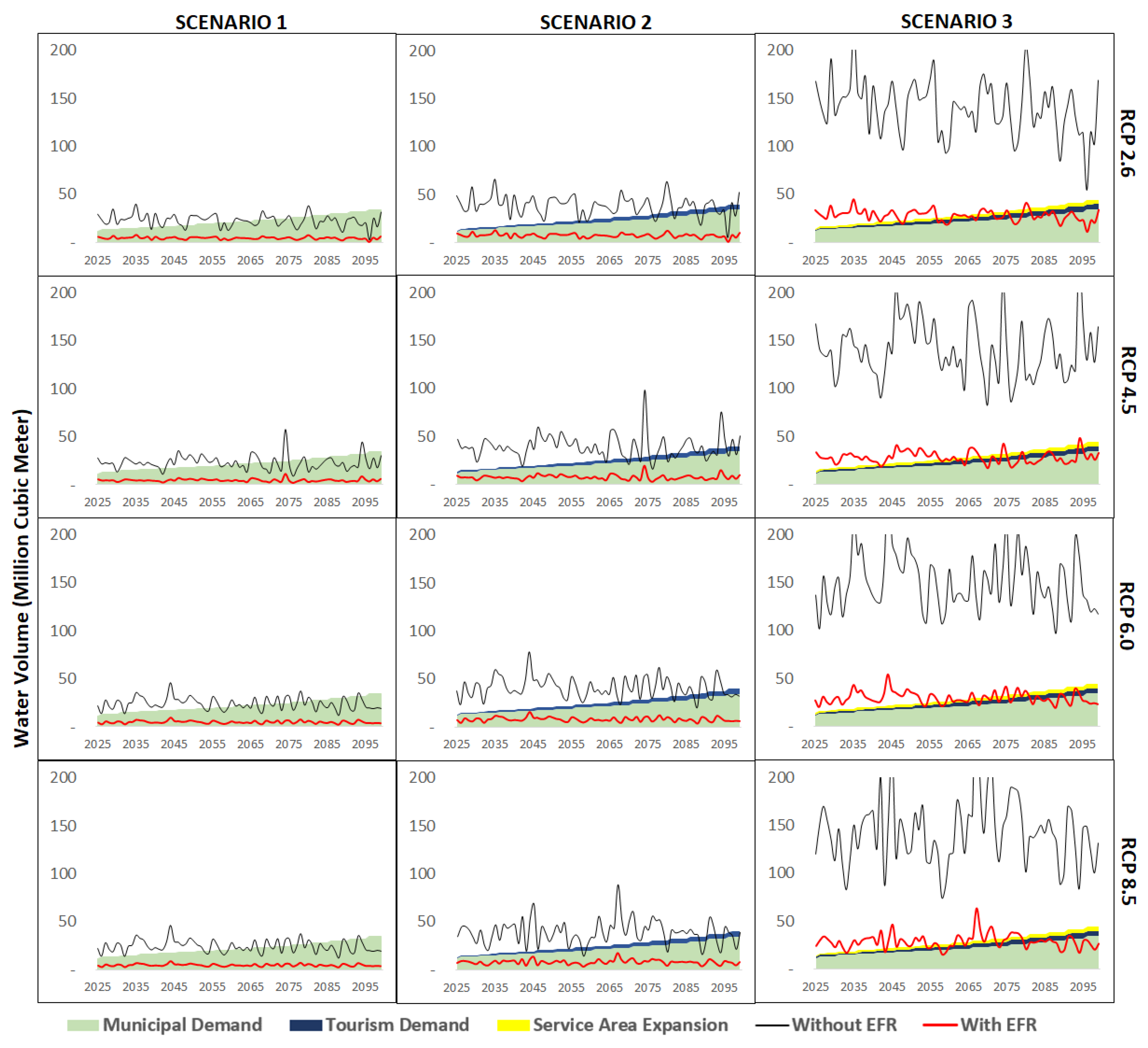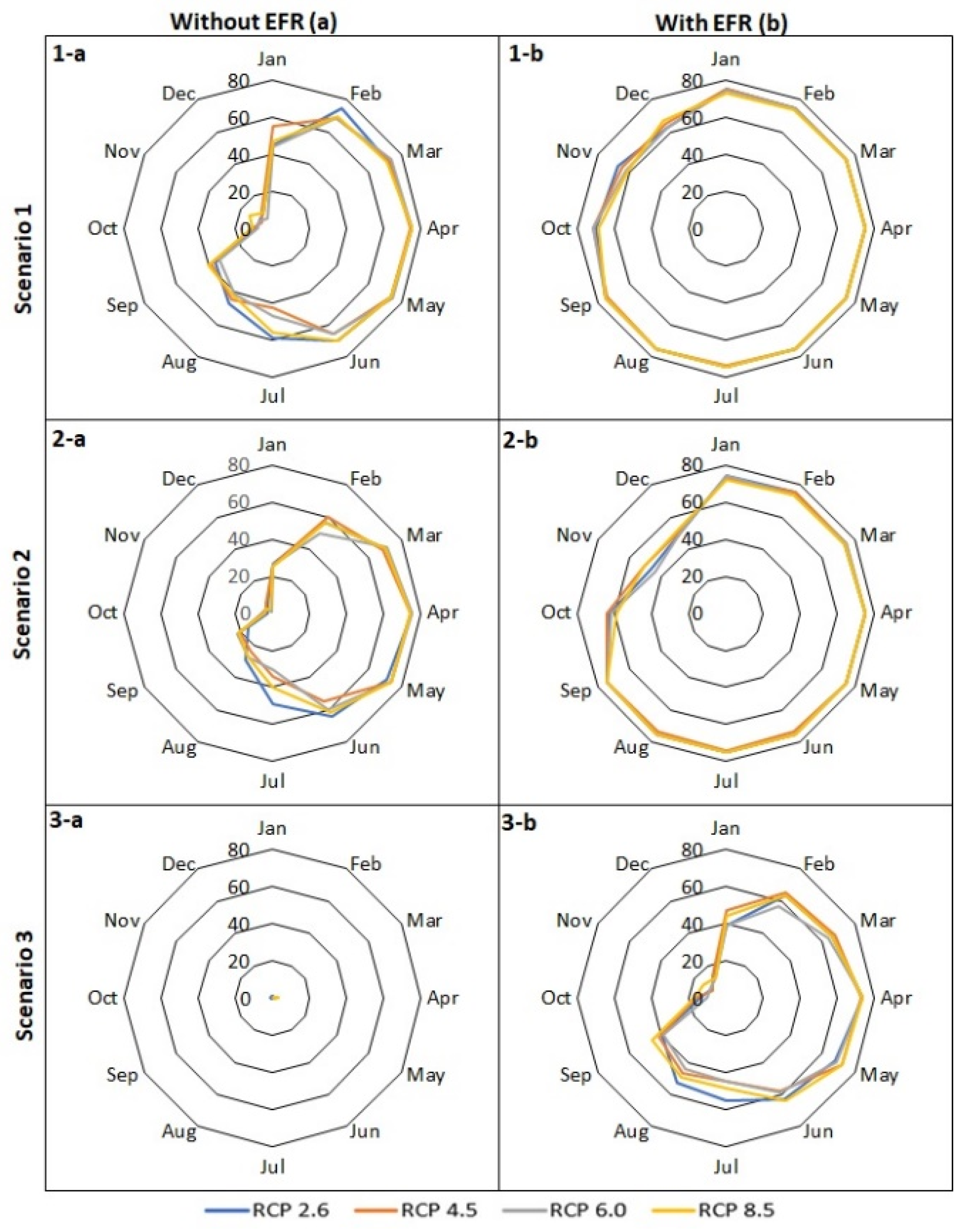The accuracy of the predicted water yield was evaluated using the Nash–Sutcliffe efficiency (NSE) and coefficient of determination (R²), and the projections of the demand models were determined using the mean absolute percentage error (MAPE). In step (3), the potential of surface-water supply, that is, sufficiency or deficiency, was assessed for the three scenarios.

3.1. Water Availability

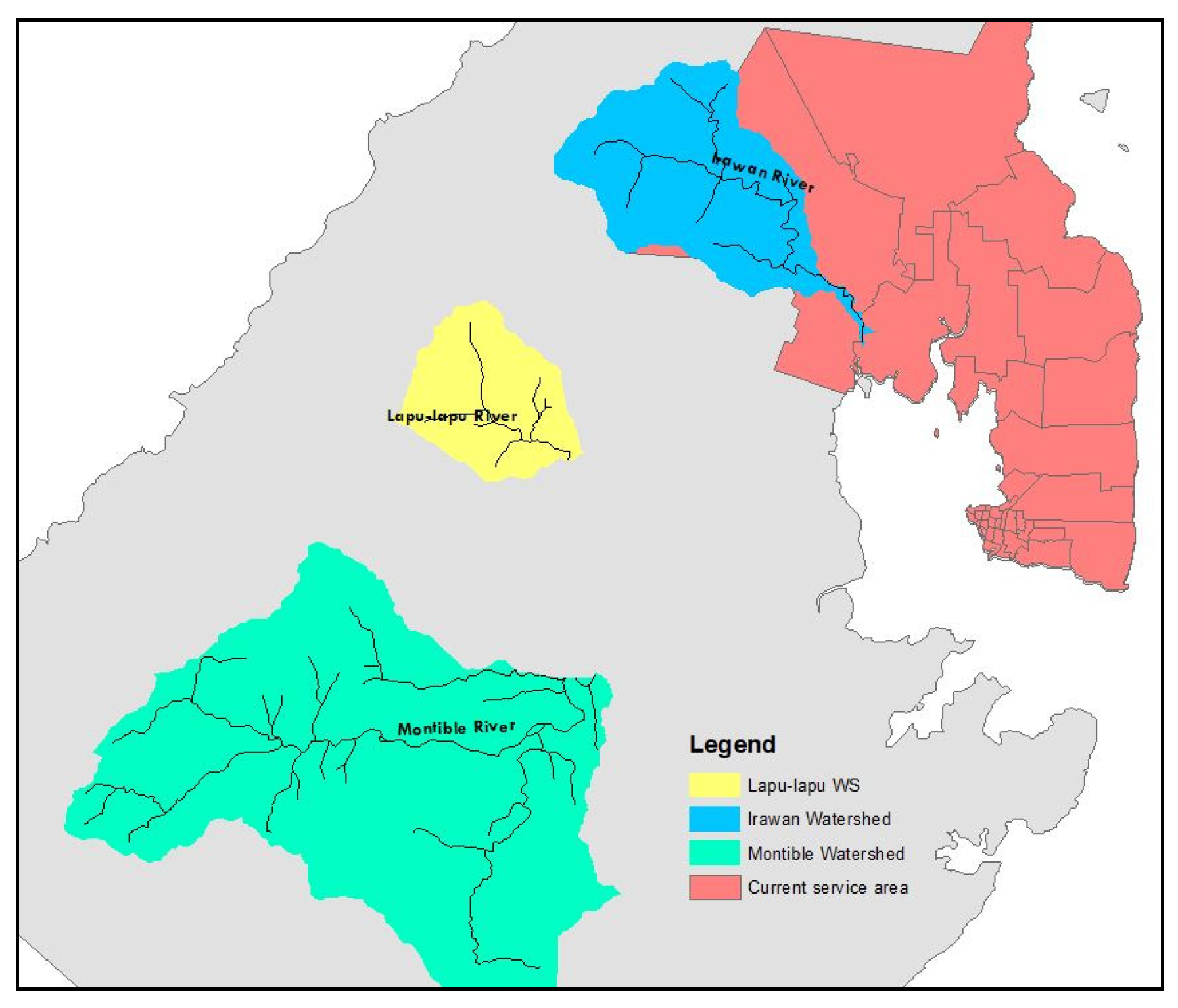
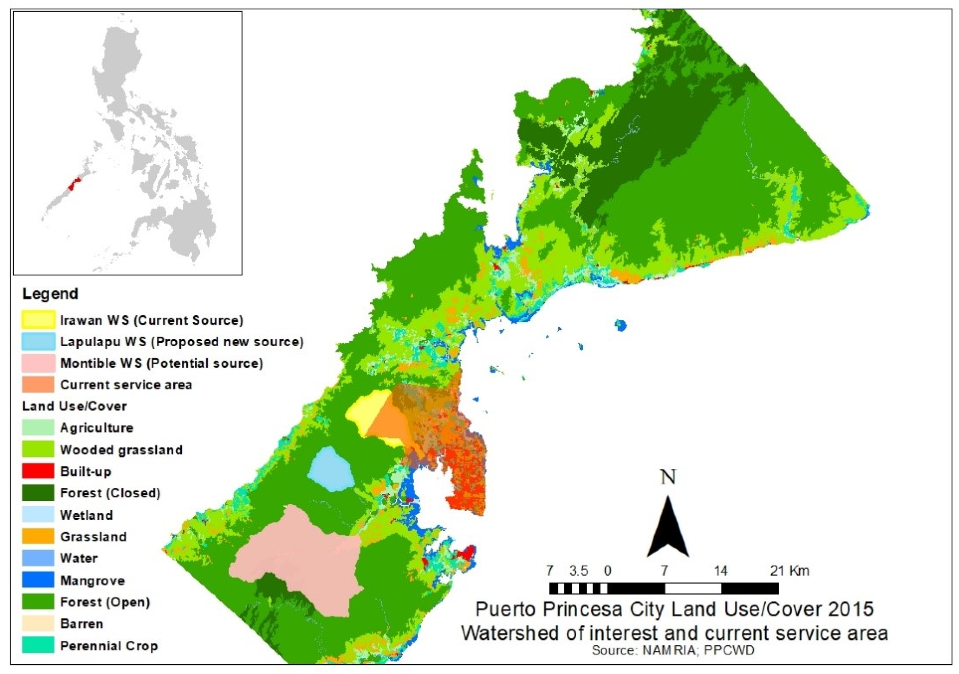
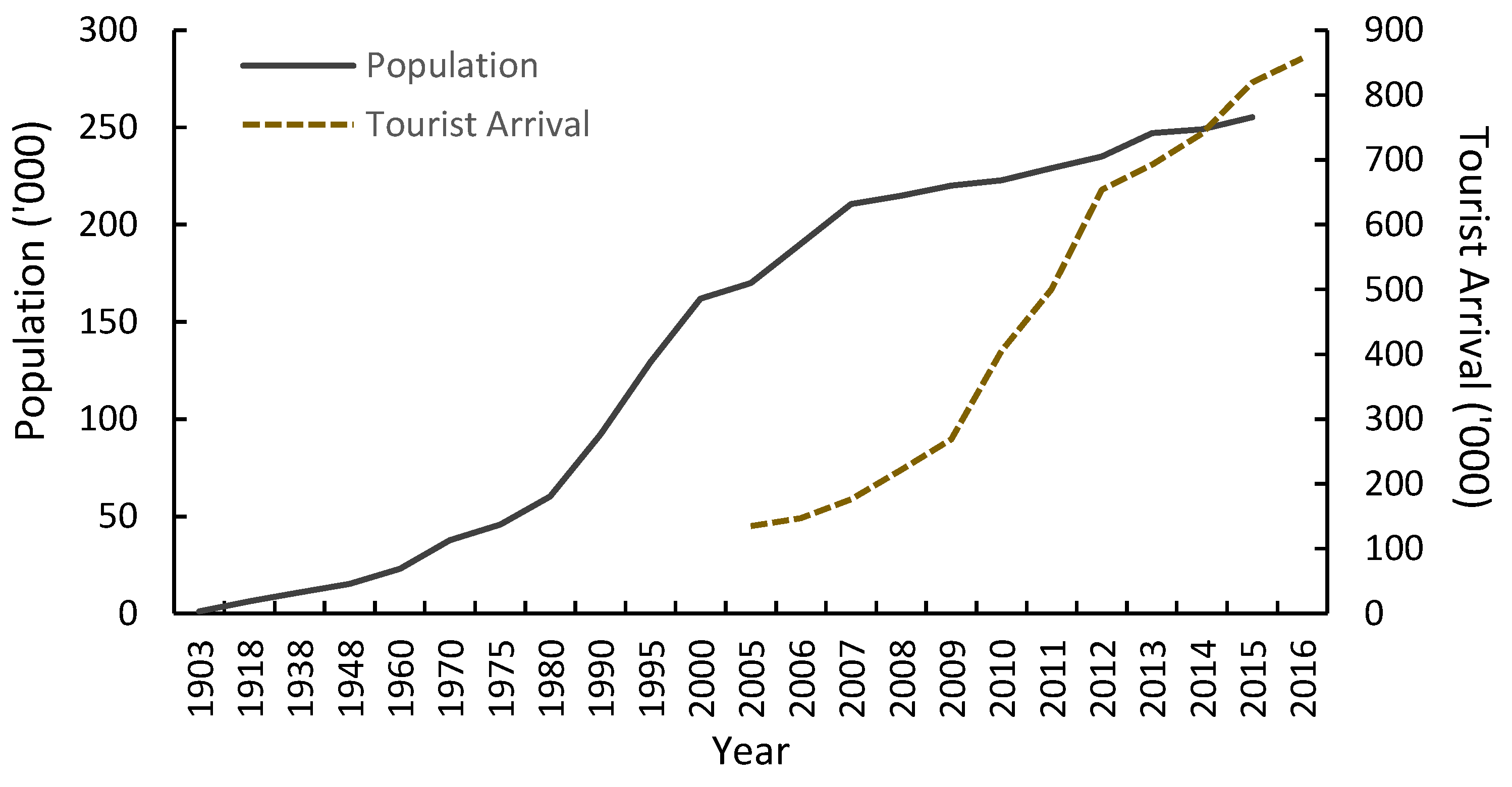
The surface water available at three watersheds (Irawan, Lapu–Lapu, and Montible) was determined using the SWAT model [21,22,23] and computed using Equation (1). Watersheds were subdivided into subbasins using a river network map (Figure 3). Despite the sudden increase in tourist arrivals since 2009, the assumptions for planning and designing water-supply systems have remained unchanged, thereby ignoring the changing water consumption patterns. Sub-basins were then further divided into hydrological response units, which consist of large areas with unique combinations of soil, land use, and slope.

$${\mathrm{SW}}_{\mathrm{t}}={\mathrm{SW}}_0+{\displaystyle \sum }_{\mathrm{i}=1}^{\mathrm{t}}\left({\mathrm{R}}_{\mathrm{day}}-{\mathrm{Q}}_{\mathrm{surf}}-{\mathrm{E}}_{\mathrm{a}}-{\mathrm{w}}_{\mathrm{seep}}-{\mathrm{Q}}_{\mathrm{gw}}\right)$$

(1)

where SW_t and SW₀ indicate the final and initial soil water contents, respectively, t is the time (days), R_day is the precipitation, Q_surf is the surface runoff, E_a is the evapotranspiration, w_seep is the water entering the vadose zone from the soil profile, and Q_gw is the return flow. The unit of all parameters is mm, and i represents the parameter value for a day.

Baseline (1980–2017) daily rainfall, relative humidity, and temperature obtained from the Philippine Atmospheric Geophysical and Astronomical Services Administration’s (PAGASA) Puerto Princesa Synoptic Station were used. The study region has only one weather station that is situated approximately 13 km away from the Irawan watershed (WS) and 21 km from the Montible WS. The future climate data obtained from the simulations of the Hadley Center Global Environment Model2–Earth System (HaDGEM2–ES) global climate model, were subjected to bias correction through the intersectoral impact model intercomparison project–fast track (ISIMIP–FT) framework [24,25], and four representative concentration pathways (RCPs) such as RCP2.6, RCP4.5, RCP6.0, and RCP8.5 were used. Additional and equally essential input data are listed in

Table A1. Input data for ArcSWAT.

Data Type	Description	Sources
Digital elevation model	SRTM 5 m × 5 m resolution	National Mapping and Resource Information Authority (NAMRIA) (pers.com.)
Land use vector	Digitized Landsat 8 (30 m × 30 m)
Soil vector	Digital Soil Map of the World v. 3.6 (1: 5,000,000)	Land and Water Development Division, FAO, Rome (http://www.fao.org/geonetwork/srv/en/metadata.show%3Fid=14116 (accessed on 14 February 2018))
Baseline climate data (1980–2017)	Daily rainfall, relative humidity, maximum and minimum temperatures (station point)	Philippine Atmospheric Geophysical and Astronomical Services Administration (PAGASA) (pers.com.)
Climate projection data (2020–2099)	Bias-corrected daily rainfall, relative humidity, maximum and minimum temperatures (0.5° × 0.5°)	HaDGEM2–ES dataset (http://h08.nies.go.jp and https://esg.pik-potsdam.de (accessed on 14 February 2018))
Hydrological data (1980–1999)	Monthly streamflow	Pennoni Associates Inc. et al., 2002 (pers.com.)
Weather generator	Weather generator generated from the PAGASA observations	Alibuyog et al., 2015 (pers.com.)

.

The first five years of the baseline and future simulations (1980–1984 and 2015–2019, respectively) were used as warm-up periods. Note that the data used for calibration (1980–1990) and validation (1991–1999) were generated using a water balance approach based on the actual observations of Pennoni et al. (2002) [26]. On the other hand, the Lapu–Lapu WS was neither validated nor calibrated due to a lack of data. The calibrated parameters from the Irawan WS were simply transferred because of its proximity and comparable topography, soil, and land use.

Automatic calibration, validation, and uncertainty analyses were performed using the sequential uncertainty fitting algorithm version 2 (SUFI-2) in the SWAT calibration and uncertainty programs package [27]. The model was evaluated using monthly discharge by computing R² and NSE values [28]. The suggested statistical thresholds are shown in

Table 1. Statistical thresholds for model evaluation and calibration [28].

Objective Function	Threshold (Streamflow)
NSE
Very good	0.75–1.00
Good	0.65–0.75
Satisfactory	0.50–0.65
Unsatisfactory	≤0.50
R2	≥0.50
T-stat	Larger absolute value
p-value	<0.05

.

In the absence of clear standards for setting EF in the Philippines, this study adopted a presumptive standard that allowed up to 20% of annual and monthly flows for alteration, maintaining 80% of flows to sustain ecological health [29].

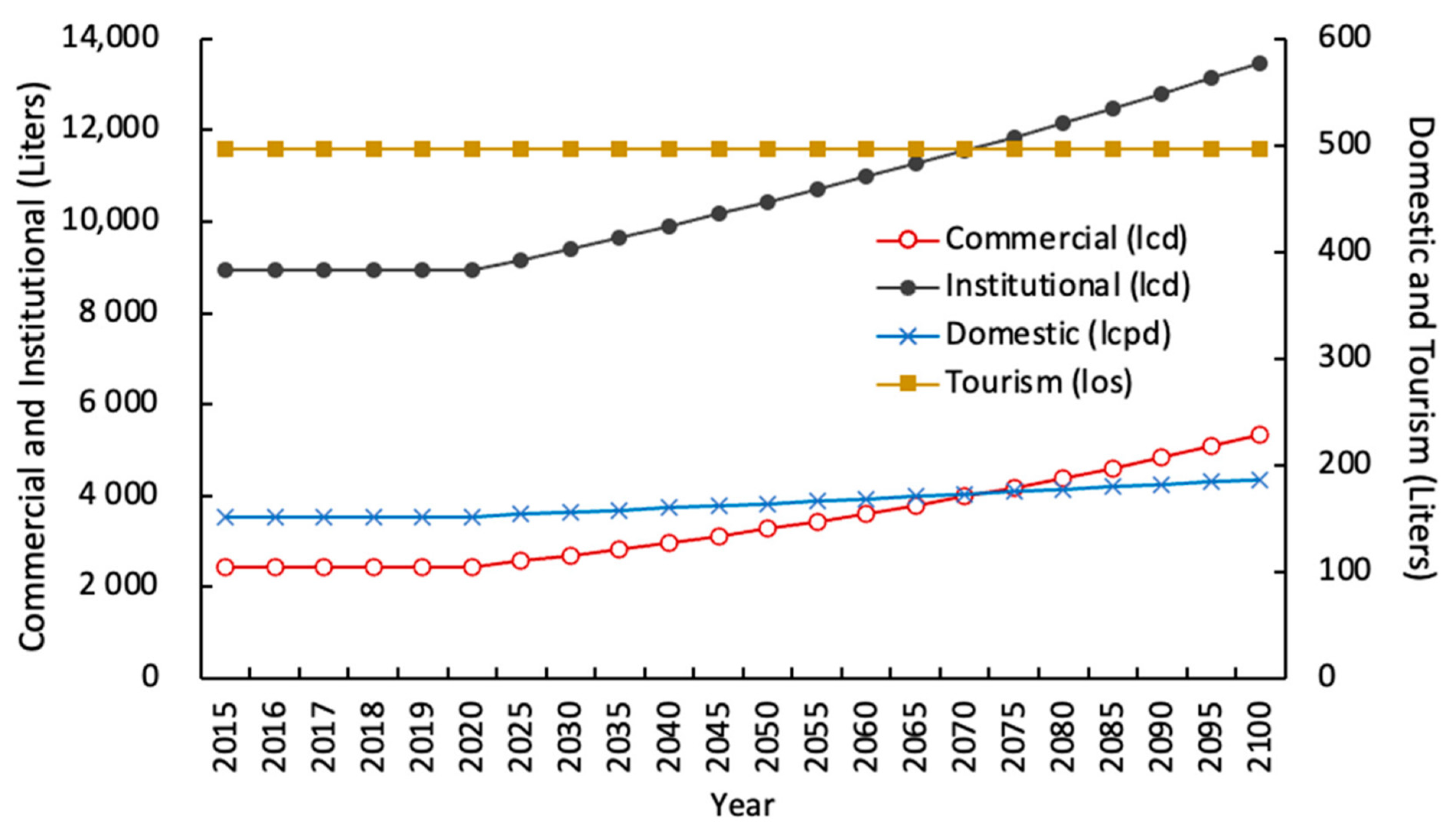
3.2. Water Demand

Population is the primary data used for determining conventional municipal water demand (domestic, commercial, and institutional demand sectors) in a service area [30]. This was projected geometrically from the 2015 census. The projected municipal growth rates used were computed using the ratio method from the projected provincial growth rates until 2045 obtained from the Philippines Statistics Authority. The absence of longer projected growth rates enabled us to use the 2045 growth rate until 2100 projections [31,32].

A stylized model [33] (Equation (2)) was used to capture the tourism sector’s water demand (corresponding to the business as usual (BAU) scenario) and to determine the total municipal demand. Each demand type was determined using Equations (2a)–(2g). Commercial and institutional consumers were determined proportionally to the population [30]. All water-use factors (WFs) were determined from consumption records. The lack of water consumption records for the year 2000 and before limited the validation to focus on demand Scenario 2 (BAU scenario) only.

$${\mathrm{TotD}}_{\mathrm{t}}={\mathrm{DD}}_{\mathrm{t}}+{ \mathrm{CD}}_{\mathrm{t}}+{\mathrm{ID}}_{\mathrm{t}}+{\mathrm{TD}}_{\mathrm{t}}$$

(2)

where TotD_t is the total water demand in the service area per unit time t (m³/t), DD_t is the domestic demand in the service area per unit time t (m³/t), CD_t is the commercial demand in the service area per unit time t (m³/t), ID_t is the institutional demand in the service area per unit time t (m³/t), and TD_t is the tourism demand in the service area per unit time t (m³/t).

Domestic demand (DD_t) is the utilization of water directly drawn from a source or supply system by a household for drinking, washing, bathing, cooking, and watering of gardens, or by animals and other domestic uses. Thus, it is entirely driven by the population and calculated using Equation (2a) [30].

$${\mathrm{DD}}_{\mathrm{t}}={ \mathrm{P}}_{\mathrm{t}}\times {\mathrm{DWF}}_{\mathrm{t}}$$

(2a)

where DD_t is the domestic demand per unit time t, P_t is the population per unit time t, and DWF_t is the domestic water use factor per unit time t. A provincial-level projected population growth until the year 2045 was obtained from the Philippine Statistics Authority (PSA), which accounts for the demographic changes occurring in each province, such as fertility, mortality, and migration. These data absent at the municipal/city level, making it impossible to use such a method. Alternatively, the population was projected using a geometric Equation (2b) by utilizing population growth rates [30]. The projected municipal growth rates were calculated using the ratio method [31,32] to that of the projected provincial growth rates from the PSA until 2045. Constant growth rates were applied for succeeding years, which is equal to the last projected growth rate (2045). The initial population was based on the 2015 census population.

$${\mathrm{P}}_{\mathrm{t}}={\mathrm{P}}_0{\left(1+\frac{\mathrm{r}}{100}\right)}^{\mathrm{t}}$$

(2b)

It is assumed that services cover 90% of the 74% population within the city in 2015 (74% of the households in 2015 resided within the service area; based on interviews with water company managers), and the services will be expanded to neighboring villages. The DWF was calculated as 152 L per capita per day (lcpd), or 0.152 m³ day⁻¹, based on the 2016 consumption records of the PPCWD. According to the Local Water Utilities Administration (LWUA) [31], this value is projected to increase by 5% every five years.

Commercial water demand (CD_t) includes all other private businesses and industries. It is determined by the number of commercial connections that can be derived from the ratio of commercial establishments to the population in the service area [30]. There is a relationship between the number of commercial–industrial connections and the service area population, which varies between 0.3 and 1.2 connections per 100 population [31]. Based on the 2016 records of the PPCWD, a ratio of 0.36 commercial connections per 100 inhabitants (excluding accommodation establishments (AEs)) was used. The commercial connections could then be used to assess the commercial water demand using Equation (2c,d) as follows:

$${\mathrm{CD}}_{\mathrm{t}}={ \mathrm{C}}_{\mathrm{t}}\times {\mathrm{CWF}}_{\mathrm{t}}$$

(2c)

where CWF_t is the commercial water use factor per unit time, t. The CWF_t is benchmarked in the year 2000 records and projected to increase by 2% annually. This year is the earliest consumption record collected, which was when the effect of tourism on commercial water consumption was still negligible (i.e., 0.17% of the population comprises daily tourists). The 2015 CWF was determined as 1.9 m³ conn.⁻¹ day⁻¹, and this value was used to predict the succeeding years with a 5% increase every 5 years [31].

$${\mathrm{C}}_{\mathrm{t}}=\frac{{\mathrm{P}}_{\mathrm{t}}}{100}\times 0.36$$

(2d)

where C_t is the number of commercial connections per unit time t, P_t is the population per unit time t, and CD_t is the commercial demand per unit time t.

The institutional water demand (ID_t) includes water requirements from schools, churches, public administration buildings, and hospitals, and it was calculated using Equations (2e,f). The underlying assumption is that there is one institutional connection per 2000 inhabitants. Based on the PPCWD 2016 records, the calculated IWF is 13.41 m³day⁻¹connection⁻¹ and it is projected to increase by 2.6% every 5 years [31].

$${\mathrm{ID}}_{\mathrm{t}}={ \mathrm{I}}_{\mathrm{t}}\times {\mathrm{IWF}}_{\mathrm{t}}$$

(2e)

$${\mathrm{I}}_{\mathrm{t}}=\frac{{\mathrm{P}}_{\mathrm{t}}}{2000}$$

(2f)

where I_t is the number of institutional connections per unit time t, P_t is the population per unit time t, ID_t is the institutional demand per unit time t, and IWF_t is the institutional WF per unit time t.

Tourism water demand (TD_t) is the consumption determined from AEs [11,12,15,34,35]. There are significant differences in water consumption depending on the type of accommodation (hotel, campsites, bed and breakfast, resort, etc.) and tourist activities. This study adopted the City Tourism Office’s (CTO) AE classification (hotels, tourist inns, pension houses, and resorts). The monthly water consumption was determined from a purposive stratified sample of 82 AEs within the service area based on the 2017 PPCWD records. Based on the CTO’s report, the average overnight stay period per tourist per AE type is 1.6 nights (the average length of stay of a tourist in the city per visit). The average tourist water consumption factor (TWF_j) at each AE type per tourist per overnight stay was then computed using a simple arithmetic mean (Equation (2h)). This value was held constant throughout the forecast period because the literature on variations in tourist water consumption was not available. The monthly and annual water consumptions were computed using Equation (2g) as follows:

$${\mathrm{TD}}_{\mathrm{t}}={\mathrm{F}}_{\mathrm{t}}\times 1.6\times {\mathrm{TWF}}_{\mathrm{j}}$$

(2g)

$$\mathrm{T}\mathrm{W}{\mathrm{F}}_{\mathrm{j}}={\sum }_{\mathrm{i}=1}^{\mathrm{n}}{\mathrm{a}}_{\mathrm{i}},\mathrm{a}=\frac{{\mathrm{WC}}_{\mathrm{jt}} }{{\mathrm{TOS}}_{\mathrm{jt}}}$$

(2h)

where TD_t is the tourism water demand per unit time t, F is the predicted number of tourists at time t, TWF_j is the tourism water consumption factor, j is the AE type, n is the total number of samples, and a is the water consumption at time t (WC_jt) divided by the total number of guest night stays at time t (TOS_jt) of each accommodation.

Tourist arrivals simulation (Equation. (3)) was first calibrated and validated using the Holt–Winters exponential smoothing curve [36] fitted to the observed monthly tourist arrivals from 2005 to 2017. A fitted curve was used to predict future tourist arrivals. The average overnight stay was determined from sampled AE occupancy records. It was then added to the conventional total simulated municipal demand and subjected to validation.

$${\mathrm{F}}_{\mathrm{t}+\mathrm{m}}=\left({\mathrm{S}}_{\mathrm{t}}+{\mathrm{mb}}_{\mathrm{t}}\right){\mathrm{I}}_{\mathrm{t}-\mathrm{L}+\mathrm{m}}$$

(3)

$${\mathrm{S}}_{\mathrm{t}}= \mathsf{\alpha }\frac{{\mathrm{y}}_{\mathrm{t}}}{{\mathrm{I}}_{\mathrm{t}-\mathrm{L}}}+\left(1-\mathsf{\alpha }\right)\left({\mathrm{S}}_{\mathrm{t}-1}+{\mathrm{b}}_{\mathrm{t}-1}\right)$$

(3a)

$${\mathrm{b}}_{\mathrm{t}}= \mathsf{\gamma }\left({\mathrm{S}}_{\mathrm{t}}-{\mathrm{S}}_{\mathrm{t}-1}\right)+\left(1-\mathsf{\gamma }\right){\mathrm{b}}_{\mathrm{t}-1}$$

(3b)

$${\mathrm{I}}_{\mathrm{t}}=\mathsf{\beta }\frac{{\mathrm{y}}_{\mathrm{t}}}{{\mathrm{S}}_{\mathrm{t}}}+\left(1-\mathsf{\beta }\right){\mathrm{I}}_{\mathrm{t}-\mathrm{L}}$$

(3c)

where y_t denotes the actual observation, S_t is the smoothed observation, b_t is the trend factor, I_t is the seasonal smoothing, F_t+m is the forecast at m periods ahead, t is an index denoting a time period, L refers to the number of data points that indicate the beginning of a new season, and α, β, and γ are constant values between 0 and 1 that must be estimated such that the error is minimized.

3.3. Integrated Supply and Demand Scenarios

Three possible scenarios, accounting for future population, climate, and tourism, were developed to assess the dynamics between water demand and supply (

Table 2. Integrated demand and supply scenarios.

	Demand Scenario	Supply Scenario
Scenario 1	Municipal Demand (Population, commercial, and institutional demand)	Irawan WS + Climate Change + with and without EFR
Scenario 2	Municipal Demand + Tourism (BAU)	Irawan WS + Lapu–Lapu WS + Climate Change + with and without EFR
Scenario 3	BAU + Tourism + Service area expansion (increased municipal demand)	Irawan WS + Lapu–Lapu WS + Montible WS + Climate Change + with and without EFR

WS = watershed; BAU = business as usual; EFR = environmental flow regulation.

). Water demand is driven by changes in the population and tourist arrivals over time. On the other hand, water supply is determined based on the simulated water yield from the current (Irawan WS) and additional surface-water sources (Lapu–Lapu WS and/or Montible WS) while maintaining or ignoring EF regulation (EFR).

To determine the level of water scarcity, water demand was compared with water availability on an annual and monthly basis [37]. The city was judged as surface-water sufficient (SWS) when the forecasted water supply exceeded the forecasted demand (demand < supply). Conversely, the city was judged as surface-water deficient (SWD) when the forecasted demand exceeded the forecasted supply (demand > supply).

4. Results and Discussion

4.1. Model Calibration and Sensitivity Analysis

Model evaluation yielded highly adequate results in the Irawan WS (NSE = 0.87, R2 = 0.88) and Montible WS (NSE = 0.88, R2 = 0.84, “Very Good (see Table 1)”) showing less error variance between the simulated and measured data. The Irawan WS was calibrated with eight parameters of high sensitivity (

Table A2. Irawan and Montible WS sensitive parameters.

Parameter Name	Parameter Full Name	Irawan WS		Montible WS
		T-Stat	p-Value	T-Stat	p-Value
R__CN2.mgt	SCS curve number	−5.32	0.00	−0.83	0.41
R__SOL_K(..).sol	Saturated hydraulic conductivity	3.95	0.00	−0.49	0.63
R__SOL_BD(..).sol	Moist bulk density	−9.63	0.00	−6.51	0.00
R__OV_N.hru	Manning’s ‘n’ value for overland flow	−2.44	0.02	−1.90	0.06
V__RCHRG_DP.gw	Deep aquifer percolation fraction	−0.24	0.81	2.92	0.00
V__SURLAG.bsn	Surface runoff lag coefficient	−0.26	0.80	0.29	0.77
V__ALPHA_BF.gw	Baseflow alpha factor	3.12	0.00	10.84	0.00
V__GW_DELAY.gw	Groundwater delay−time	−0.72	0.47	2.40	0.02
V__GWQMN.gw	Groundwater minimum threshold	0.21	0.83	0.66	0.51
V__GW_REVAP.gw	Groundwater revap coefficient	−0.45	0.65	0.09	0.93
V__ESCO.hru	Soil evaporation compensation factor	−4.28	0.00	−2.71	0.01
V__CH_N2.rte	Manning’s ‘n’ coefficient	−3.06	0.00	−3.09	0.00
V__CH_K2.rte	Effective hydraulic conductivity in the main alluvium channel	−6.96	0.00	−8.45	0.00
R__SOL_AWC(..).sol	Available water capacity of the layer soil	−0.22	0.82	1.34	0.18

) that belong to soil, groundwater, evapotranspiration and time of concentration, surface runoff, and channel processes. The Montible WS, on the other hand, was calibrated with seven parameters of high sensitivity (Table A2) that belong to soil and groundwater processes, channel processes, and evapotranspiration.

Neither measured nor simulated discharge data were available for the Lapu–Lapu WS. Similarities to the Irawan WS based on land cover, soil type, and topography were observed. Thus, the sensitive parameters for the Irawan WS were used in calibrating the Lapu–Lapu WS.

4.2. Water Availability Considering Climate Change and Environmental Flow

The annual average minimum and maximum temperatures will decrease in RCP2.6 and increase in other RCPs, compared to the baseline (

Table 3. Annual mean of historical and projected climate variables.

	Baseline	RCP2.6	RCP4.5	RCP6.0	RCP8.5
Rainfall (mm)	1549.0	1734.0	1756.0	1708.0	1781.0
Min. Temperature (°C)	24.7	24.6	25.0	33.0	33.8
Max. Temperature (°C)	32.6	32.4	32.8	33.0	33.8
Relative Humidity (%)	74.0	72.0	72.0	83.0	72.0

). Dry months (February to April) will continue to be dry (driest in April), while the wet season will be wetter in all watersheds (wettest from October to December; see Figure 4). The projected increase in rainfall occurs during the wettest months, during which extreme rainfall events typically occur, which is consistent with global and regional studies [38,39]. Evapotranspiration is highest during the wet season and lowest in the dry season in all of the three WSs possibly because the wet season offers enough soil moisture so that plants can transpire close to their potential rate. Eventually, ET will reduce due to a shortage of water during the dry season; then, soil moisture is consumed [40].

The annual water yield is projected to increase for all RCPs in the three WSs possibly because of the projected increase in rainfall. The water yield increase was significant for all RCPs in the Irawan WS; in RCP2.6, and RCP6.0 in the Lapu–Lapu WS, and RCP2.6, RCP6.0, and RCP8.5 in the Montible WS (

Table 4. Results of chi-square test of water yield in the target watersheds and RCPs. The significant threshold for the p-value is less than 0.05. The filled-in boxes are nonsignificant values.

Watershed	p-Value (Significance < 0.05)
	RCP2.6	RCP4.5	RCP6.0	RCP8.5
Irawan WS	0.002	0.007	0.000	0.024
Lapu–Lapu WS	0.007	0.124	0.027	0.071
Montible WS	0.011	0.059	0.005	0.016

). A large fraction of the water yield originates from the baseflow (lateral + return flow), with minimal contribution from surface runoff (Figure 4). This is pronounced in the Montible WS, which is also less affected by seasonality, indicating a reliable water source in the present condition and in the future. This is possibly due to the fact that the Montible WS has a larger drainage area with less rugged terrain; hence, it has a higher potential for storing water for baseflow. During the dry months, the projected increase in the mean monthly water yield in the Montible WS was relatively stable up to April, compared to the Irawan and Lapu–Lapu WSs, where it occurred only until February (Figure 4b). Likewise, baseflow was highest in the wet season and lowest during the dry season (March–May) in all WSs (Figure 4c).

The potential water availability increases with climate change. However, to maintain EFR, the annual average water availability dramatically decreases by 80% at 3.78–4.83 Mm³ in Scenario 1, 6.40–8.20 Mm³ in Scenario 2, and 23.31–30.13 Mm³ in Scenario 3 (

Table 5. Annual water yield for each supply scenario.

Watershed Source	Without EFR					With EFR
	Baseline	RCP 2.6	RCP 4.5	RCP 6.0	RCP 8.5	Baseline	RCP 2.6	RCP 4.5	RCP 6.0	RCP 8.5
Supply Scenario 1: Irawan WS
Mean	18.87	22.66	22.95	24.16	23.09	3.78	4.53	4.59	4.83	4.62
Minimum	6.33	2.49	8.71	11.95	8.35	1.27	0.50	1.74	2.39	1.67
Maximum	44.06	39.74	57.87	46.39	52.10	8.81	7.95	11.57	9.28	10.42
Supply Scenario 2: Irawan + Lapu–Lapu WS
Mean	31.98	38.49	39.00	41.02	39.24	6.40	7.70	7.80	8.20	7.85
Minimum	10.72	4.94	15.49	20.33	14.42	2.14	0.99	3.10	4.07	2.88
Maximum	74.72	66.29	98.01	78.55	89.12	14.94	13.26	19.60	15.71	17.82
Supply Scenario 3: Irawan + Lapu–Lapu + Montible WS
Mean	116.48	140.21	141.36	150.54	143.98	23.31	28.06	28.29	30.13	28.81
Minimum	46.01	54.19	83.31	98.20	74.91	9.20	10.87	16.66	19.69	14.98
Maximum	240.88	224.00	243.89	273.07	317.91	48.18	44.80	48.78	54.76	63.58

). As a result, for Scenarios 1 and 2, the dependency on groundwater will remain inevitable in the immediate future.

4.3. Social Changes and Water Availability

The estimate of tourist arrivals achieved through simulation is rather accurate (MAPE = 7.7%) and was used to validate the stylized model for demand Scenario 2 (where MAPE is 5.7%). Tourist arrivals are likely to increase as the municipality expands its connectivity to other major islands in the country and to other countries. Along with this, water demand is also expected to skyrocket and potentially compete with the domestic water demand. In 2016, the water demand of a tourist for a one-night stay was equivalent to the water demand of three locals per day (Figure 5). Note that tourist water use is rather underestimated as hotels rely heavily on private wells for supply and do not disclose the amount of water pumped. Therefore, 8% of the projected societal demand is from tourists and this is projected to increase to 13% by 2100. Moreover, the expansion of the service area will account for 10% of the projected societal demand during the entire projection period, as illustrated in Figure 6.

4.4. Integration and Water Availability

The dynamics of water availability, cumulative changes in society, climate change, and the imposition of EFR are expressed as SWS or SWD throughout the 75-year simulation (Figure 6). When the EFR is maintained, no SWS is possible during the entire simulation period for all scenarios. In addition, SWS is only frequent during the first half of Scenario 3 (53% of the simulation period). Achieving a sustainable water supply by fulfilling the municipal demand while maintaining the EF can only partly be achieved by the contribution of the Montible WS as a water source. Without EFR, it becomes easier to reach SWS, and the target is met by 48%, 83%, and 100% in Scenarios 1, 2, and 3, respectively (Figure 6 and

Table 6. Number of surface-water sufficient (SWS) years during the projection period (2025–2100) for different scenarios.

Scenario	With EFR				Without EFR
	RCP2.6	RCP4.5	RCP6.0	RCP8.5	RCP2.6	RCP4.5	RCP6.0	RCP8.5
1	0	0	0	0	36	36	36	36
2	0	0	0	0	64	59	63	65
3	39	40	40	40	75	75	75	75

). Given the current agenda of the PPCWD, despite the planned addition of the Lapu–Lapu WS as an additional surface-water source, the municipality will still suffer from a lack of surface-water supply, and therefore, groundwater will remain a significant contributor to water supply in the service area.

The seasonal evolution of the surface water deficit (SWD) is displayed in Figure 7. The larger the web, the longer the municipality will experience SWD. As expected, prominent periods of SWD are concurrent with the dry season (except in Figure 7(3-a)). Considering EFR, SWD will be experienced almost throughout the year in Scenario 1 (97%) and Scenario 2 (92%). In Scenario 3, the SWD is projected from February to September. Without EFR, the SWD decreases to 63%, 51%, and 0.01% for Scenarios 1, 2, and 3, respectively. Again, heavy reliance on groundwater extraction is expected during the SWD months.

The need to conduct studies to determine proper EFs for each watershed cannot be overemphasized. EFR refers to (1) recognizing that there is a physical limit beyond which a water resource suffers irreversible damage to its ecosystem functions and (2) systematically balancing the multiple water needs of the society in a transparent and informed manner [41]. This must be determined by science and through social decisions.

5. Conclusions

The overall methodology presented in this paper serves as a tool for improving water supply planning practices and updating conventional practices, especially for areas with booming tourism industry. It considers (1) scenarios of seasonal droughts to prepare for climate risks in the future and (2) scenarios of water availability that do not depend on groundwater supply, in which the projected deficiency is frequent both annually and seasonally. For our case study, additional water supply from the Montible WS for the PPC was projected to secure sufficient amounts of water to achieve SWS, which is consistent with the goals of both the municipality and the water company to reduce the dependency on groundwater. Significant investment costs in infrastructure must be anticipated in Scenario 3 because of the proximity to the existing water system.

The proposed integrated approach allows water managers to predict the future of surface-water sufficiency/deficiency in a region with active tourism. It also captures both sustainable and unsustainable options for water development from the perspectives of climate and social changes. Thus, this integrated approach can be used to pursue sustainable water resource development provided that a site-specific EFR is determined. However, there is no panacea for challenges in water-resource planning. Site-specific patterns exist in the consumption and nature of potential water resources. The efficiency of the water distribution system and its effect on water yield may be integrated in future studies for further model improvement.