A Sequential Optimization Approach in Tactical Planning for Value Creation in the Forest Products Industry

Abstract

Strategic, tactical, and operation-level forest management plans are commonly formulated by forest planners following even-flow yield principles. Although strategic planning ensures a sustained supply of timber over the long term, it disregards individual mills’ requirements, which leads to discrepancy between supply and demand. We hypothesize that a value-based timber allocation decision, which accounts for individual mills’ demands during tactical level planning, reduces such discrepancy by increasing value over the entire supply chain. Three types of linear programming models were constructed: Model A—status quo volume-maximization model, Model B—supply chain net present value-maximization (NPV) model, and Model C—a novel approach with sub-models embedded that maximize the NPV of individual mills in the allocation decision. Our results showed that only 58% of the annual allowable cut was profitable and the mean net revenue per harvested area was $2455 ha⁻¹ using Model A. The respective values using Models B and C were 64% and $3890 ha⁻¹ and 96% and $4040 ha⁻¹, respectively, showing that Model C generated the highest net revenue for all mills. Such a method of value-based sequential optimization (Model C) will be crucial in sustainable use of forest products and sustaining future bioeconomy, particularly for managing mixed species stands that contain timber suitable for manufacturing a wide range of products with different market values.

1. Introduction

Forest management planning outlines a set of activities to be employed to meet landowner objectives over a long-term planning horizon [1]. Linear programming (LP)-based models have been used as decision support tools to develop strategic management plans in commercial forests since the 1960s [2]. LP, with two model forms, namely Model I and II, formulated by Johnson and Scheurman [3], is a widely used model in strategic harvest planning. A third model form, named Model III or network flow model [4,5], is also used in forest planning. These models are formulated to achieve sustained harvest flow and sustainability of forest ecosystems [6].

There is a hierarchy of forest management plans (strategic, tactical, and operational) based on the spatial and temporal scales of planning activities [6,7]. Strategic planning of timber production is usually executed over a time period equivalent to one and a half forest rotation cycles, e.g., 150, 200 years [8,9] or longer to allow future managed stands to realize their growing potential. Strategic planning focuses on providing a sustained yield of timber considering the vulnerability of risk to landscape, forest ecosystem, and biodiversity. As such, it intends to maximize annual allowable cut (AAC) of merchantable timber volume abiding by sustained yield (volume) principles [6]. Subsequently, economic attributes of forest management are considered at the tactical planning level. The time horizon of tactical planning may vary from 1 to 20 years [7,10]. Finally, the operational level is where the forest management plans are executed. Therefore, operational plans deal with much smaller spatial scale (individual stand or even individual tree), a short time scale (daily, weekly, or monthly activities), and detailed economic information [11]. As such, operational-level plans outline harvesting activities such as felling, bucking, transportation, road construction, and other silvicultural activities [11,12].

On the other hand, the industrial stakeholders have their own hierarchical planning framework focused on wood procurement, production, distribution, and the sale of forest products [12,13,14]. The industrial strategic plan is mainly guided by an objective of maximizing economic value, attempting to achieve a stable wood supply [2,5]. Consequently, the industrial plan is concerned with location/acquisition of new mills, selecting product type, investment, and market development [12,15]. The time horizon for an industrial strategic plan is generally less than 20 years [16]. The tactical plan focuses on determining areas for harvesting, logging, transporting, and managing other inventory activities [17]. Its time horizon ranges from a week up to a year [12,17,18,19,20]. Finally, the operational level focuses on daily to weekly scheduling and production and delivery planning [12]. Overall, the time horizon of each planning hierarchy is much shorter than that of forest management planning.

Forest management planning needs to incorporate industrial fiber demand to sustain the forest-products-based industry and bioeconomy [5,21,22]. Moreover, an industrial ecosystem and efficiency are also equally important attributes in industrial planning that promote a green circular economy and sustainability of the wood industry [20]. However, it is a challenge to synchronize forest management planning and industrial planning due to the differences in the objectives and time horizons used in these two frameworks [5,10,12,16,17]. In practice, this incorporation of industrial fiber demand is attempted only at the tactical or operational planning levels. The plans are developed in a hierarchical manner, i.e., forest management plans are developed first, followed by the development of wood procurement plans for forest products supply chains. Forest management planning is considered the upper hierarchical level, and forest products supply chain planning is considered the lower level; both acting independently in their decision processes [23,24]. There are a number of planning models designed for industrial fiber demand and procurement, but they tend to ignore long-term forest sustainability [10,25]. Similarly, forest management planning models usually do not explicitly consider industrial fiber values. Specific product recovery potentials are not taken into account, but different types of logs (e.g., species, diameter, form factor, etc.) of the same volume will produce different amounts of final products [26,27]. A factor that may have contributed to this lack of integration is the differences in value systems between managing forests, which focuses on ecological and social services [6,28] and operating forest-based industries where the focus is on economics [12,22,29]. Recent studies have demonstrated the need to develop harvest plans that explicitly take into consideration industrial requirements a priori, using integrated planning approaches [29,30,31].

The sustained yield harvest principle that maximizes timber volume is a deep-rooted planning policy in Canada. It is evident in timber harvest license agreements (TLA) granted to forest industries [9,32] where harvest scheduling contracts are made in terms of timber volume [9,33]. There may be more than one TLA wood mill in a single forest management jurisdiction, called a forest management unit (FMU). The economic value of forest products stemming from the same FMU can vary depending on product recovery potential by a specific mill for the specific species and transformed products [26,34]. When TLA requirements are not incorporated into the forest management planning process, the supply of wood for mills may be jeopardized. The available harvest volumes may exceed one mill’s demand, whereas another mill may face demand deficit. In order to reduce such a gap, Cantegril et al. [35] proposed searching alternative markets for underused timber. Finding an alternative market can maximize the use of AAC volumes, but the economic return can be suboptimal if sent to a low-value producing mill. Paradis et al. [36] proposed a hierarchical bi-level planning model that either reduces the timber harvest or harvests only the amount that is commercially demanded. When managing mixed wood forest stands, decisions based on the value of one assortment will influence another assortment. It may not be financially viable to procure just a selected assortment without being able to deliver all assortments to its highest value-yielding mills, hence reducing overall supply chain profit. In such a context, a vertically integrated model can make better allocation decisions, increasing overall supply chain profit [22,30]. Such an integrated model compensates one mill’s loss with another mill’s profit. Although this is theoretically attainable, it will not be practical because mills are independent entities with their own decision-making structure and interests [37], unless they belong to the same company.

We hypothesize that a better coordination between strategic (AAC calculation) and tactical planning (harvest scheduling and financial analysis) of timber harvest can increase overall forest value. Value refers to economic returns from manufactured products. Better coordination can be achieved by taking into consideration product-wise (e.g., species-specific sawlogs, pulp logs) demand and aligning it with supply during tactical planning. Allocating volumes sequentially starting from high-value to low-value products will lead to more efficient supply of timber by (a) reducing the discrepancy between demand for and supply of each TLA mill, (b) increasing the profitable supply of wood for each mill, and (c) reducing the unprofitable timber harvest. The objectives of this study were to (i) evaluate the economic performance of our novel planning approach as compared to other models currently utilized and (ii) examine the impact of implementing the new planning approach on the sustained flow of high-value timber over the planning horizon.

2. Methods

Timber harvest scheduling optimization model solutions outline periodic allowable cuts, taking into consideration site-specific forest growth and management objectives. One of the key objectives of the public forest for timber production is to produce economically profitable timber while considering the site-specific forest ecosystem and biodiversity conservation. We formulated three timber harvest scheduling models (

Table 1. A synthesis of three models and their important features.

Scenario	Assigned Model Name	Objective Function	Important Constraint	Time Horizon
Base case	A	Total harvest volume	Even flow of harvest volume	30 Periods
NPV	B	Net present value from all products	Even flow of harvest volume	30 Periods
SeqNPV	C	Net present value from individual products	Even flow of harvest volume. Even flow of high-value timber harvest volume	1 Period

); all were based on a linear programming framework. Among the three models, the first one, “Model A”, is a traditionally used model based on sustained yield principles. It maximizes allowable cut ensuring even flow of the harvest volume per period for the entire planning horizon. We considered this as the base case scenario. The second one, “Model B,” is an integrated model that is also formulated based on sustained yield principles that maximizes net present value (NPV) globally for the supply chain [5,31]. This model may prescribe highly profitable flow of one product at the expense of another product, creating an uneven flow of fiber products between periods [22]. For a certain product type, harvest volume may exceed demand, whereas another product type may have supply shortage [35,36]. The third and our proposed “Model C” intends to sequentially fulfill demands from all mills based on the value of the product they generate. This model is different from Models A and B in its formulation. The key difference is that if the demand of the highest-value mill is already met, or harvest is not profitable for that mill, Model C allows the product to flow towards the next best alternative. Unlike Model B, Model C specifies the minimum quality of timber required for individual mills. Mathematical formulations of these models with added explanations are presented in Section 2.1.3.

2.1. Linear Programming Model for Timber Harvest Planning

As the simplest formulation of a forest product supply chain, we considered only two stakeholders, namely, a forest owner (government in our case) and a group of primary processing wood mills (private investors) that are associated with the forest for timber procurement. We used a stratum-based timber harvest scheduling model in order to better differentiate the growth and yield potentials of the forest stands and costs associated with distances and geography-based variations. We present the general model structure in this section and data-specific description in Section 2.3.

Sets

• S set of strata or harvest nodes
• A set of age class
• T set of planning horizon
• G set of species
• M set of wood mills or processing nodes
• P set of products

Decision variables:

• $h_{sat}$ Area (ha) planned to be harvested in age class a of stratum s and period t
• $x_{sat}$ Stand area (ha, that is assigned for timber production) of age class a in stratum s at the start of period t (ha), ∀ s, a, and t. $x_{sa0}$ is the initial area parameter before our simulation starts. $x_{sat}$ are successively generated using area accounting constraints (Equations (4)–(6) below) based on the preceding harvest ($h_{sat}$).

Parameters:

• $v_{sga}$ Timber volume in stratum s of species g belonging to age class a (m³ ha⁻¹).
• $v{p}_{sgpa}$ Product volume (p: veneer (only from hardwood), lumber, and pulpwood) recovery from timber of species g, stratum s, and age class a (m³ ha⁻¹).
• $r_{sgpa}$ Price of product p from species g harvested in stratum s of age class a ($m⁻³).
  $c_{sgpa}$ Cost (total expenditure that consists of forest management, harvesting, loading, forwarding, and road transportation) of product p from species g that is harvested in stratum s of age class a ($m⁻³).
• $a_{min.s}$ Minimum harvest age of stratum s.

2.1.1. Model A (Business as Usual)

In forest management planning of public forests in Canada, forest owners make a long-term strategic plan by maximizing timber harvest volume following sustained yield principles (e.g., [9]). This model does not incorporate any information on demand, timber quality, and capacity of TLA wood mills. In this study, this is referred to as the business-as-usual model. The mathematical formulation of the model is as follows.

$$Max z_{vol}={{\displaystyle \sum }}_{s\in S}{{\displaystyle \sum }}_{g\in G}{{\displaystyle \sum }}_{a\in A}{{\displaystyle \sum }}_{t\in T}{h}_{sat}\left(v_{sga}\right)$$

(1)

Following the sustained yield principle, we constrained the model to ensure even flow of harvest volume for all $g\in G and t\in 2\dots \max \left(T\right)$ by period, as:

$${{\displaystyle \sum }}_{s\in S}{{\displaystyle \sum }}_{a\in A}{h}_{sa\left(t - 1\right)}\left(v_{sga}\right)={{\displaystyle \sum }}_{s\in S}{{\displaystyle \sum }}_{a\in A}{h}_{sa\left(t\right)}\left(v_{sga}\right)$$

(2)

The harvested area must be less than or equal to the total productive area available in each stratum, age class, and period:

$$h_{sat}\le x_{sat},\forall s\in S,a\in A \mathrm{and} t\in T$$

(3)

Using the initial area ($x_{sa0}$) and harvest in the successive periods, the available area was generated by employing area accounting constraints in network model structure [6], as below (Equations (4)–(6)):

The youngest age-class stands regenerate immediately after harvests take place. We assumed that stands following the harvest events self-regenerated without any regeneration delay.

$$x_{s1t}={{\displaystyle \sum }}_{a=1}^A{h}_{sa\left(t - 1\right)}, \forall \mathrm{s}, \mathrm{a}, \mathrm{and} \mathrm{t} \in \{2\dots \mathrm{T}\}$$

(4)

We applied a ceiling on the stand age class that can be attained to a maximum value of A (max(A)), so that the preceding age class (A−1) moves to the sinking age class A, but age class A remains in the same age class in the subsequent period as:

$$x_{sAt}={{\displaystyle \sum }}_{a=\left(A - 1\right)}^{\mathrm{A}}{x}_{s\mathrm{a}\left(t-1\right)}-{{\displaystyle \sum }}_{a=\left(A - 1\right)}^{\mathrm{A}}{h}_{s\mathrm{a}\left(t-1\right)}, \forall s \mathrm{and} t\in \{2\dots \max (\mathrm{T})\}$$

(5)

In the same way, the intermediate age classes of the stand area between 2 and A−1 move to the successive age class in the next period if the stand is not harvested in the preceding period, as:

$$x_{sat}=x_{s\left(a - 1\right)\left(t-1\right)}-h_{s\left(a - 1\right)\left(t-1\right)}, \forall s, a \in \{2\dots \max (\mathrm{A})-1\} \mathrm{and} t\in \{2\dots \max (\mathrm{T})\}$$

(6)

Clear-cut with protection of advanced regeneration and soil, called “Coupe avec protection de la Régénération et des sols (CPRS),” is the common harvesting method in the case of commercial forest management in Quebec, Canada [38]. This is equivalent to the classical clear-cut system, except for protection of regeneration and soil with the use of light harvest machines. However, selection harvest is applied in some (predefined) of the strata. We employed a rule that any stand is eligible for selection harvest if it contains the total merchantable timber volume between 125 m³ha⁻¹ and 275 m³ha⁻¹. These lower and upper limits were set as fixed parameters following the current practice of the “Bureau du forestier en chef” (BFEC: the provincial government agency for forest management) in our study region. Depending on the geography and species richness, BFEC has determined a few strata that require partial harvest. The following constraints were implemented to filter the stands that were assigned for selection harvest (applied in predefined strata and maintained over the planning horizon):

$${{\displaystyle \sum }}_{g\in G}{v}_{sga}>=I_s\left(125\right)\hspace{1em}\hspace{1em} \forall s\in \mathrm{S} and a \in \mathrm{A}$$

(7)

$${{\displaystyle \sum }}_{g\in G}{v}_{sga}\left(I_s\right)<=275$$

(8)

where $I_s$ is an indicator for selection cut or clear-cut for stratum s. In addition, as our objective was to implement the existing strategic planning (AAC calculation), we constrained the model not to exceed predetermined AAC already calculated by the government for the forests.

Our principal research question was to search opportunities of value potential in terms of net economic profit (we often use net revenue, i.e., net revenue as the difference between revenues and costs) that would be generated by the harvest and sale of the timber as prescribed by the harvest planning model solution. In this analysis with Model A, although it does not account for economic losses or gains while modeling, we evaluated cost and benefit of the harvest prescriptions after the optimal solution (timber volume) was generated. Product wise (gp, species group-specific product), undiscounted net revenue ($Re{v}_{sat\_gp}$) [39] for the supply chain was calculated as:

$$RevMod{1}_{sat\_gpt}=h_{sat}\left(v{p}_{sa\_gp}\left(r_{sat\_gp} - c_{sat\_gp}\right)\right)\hspace{1em} \forall s, a \mathrm{and} t$$

(9)

2.1.2. Model B (Global NPV Maximized Integrated Model)

A vertically integrated model that maximizes global net present value over the supply chain has been explored since the 1980s as a way to link forest management plans and wood industry requirements [5,21]. The modeling approach has not gained traction in practice (such as in [40]). Nevertheless, it continues to be researched for its applicability [29,30,31,41]. We examined the performance of this model from a supply chain perspective. The NPV was determined for post-manufactured products sold in the market. In order to formulate this model, one more parameter was added, as follows:

$${\gamma }_p\hspace{1em}\mathrm{Periodic} \mathrm{discount} \mathrm{factor} (={(\frac{1}{1+r})}^{5t - 2.5})$$

where r is the annual discount rate. The discount factor is applied at the mid-point of a 5-year planning horizon.

The objective function of this model is:

$$Max z_{NPV}={{\displaystyle \sum }}_{s\in S}{{\displaystyle \sum }}_{g\in G}{{\displaystyle \sum }}_{p\in P}{{\displaystyle \sum }}_{a\in A}{{\displaystyle \sum }}_{t\in T}{\gamma }_t\left(h_{sat}\right)(r_{sat\_gp} - c_{sat\_gp})\left(v{p}_{s{a}_{gp}}\right)$$

(10)

subject to the same set of constraints as in Model A (Equations (2)–(8)). From the NPV-maximized model solutions, we calculated undiscounted net revenue [39] by age class of harvested volume in each stratum and period using Equation (9).

2.1.3. Model C (Sequential NPV Maximized Integrated Model)

In mixed forest stands, when we maximize the total net revenue (NPV) ensemble using Model B, there may be over-harvest of certain species to generate high net revenue, whereas mandatory harvest of another species can create negative net revenue. Consequently, this approach may favor one mill that produces a certain type of product, but the model prescription may not be favorable for another mill that manufactures a different product. This happens because different mills take different timber species as their raw materials and produce different transformed products. Therefore, we designed the third model, “Model C”, which maximized the NPV of each mill that transforms timber into various products. We embedded sub-models within the integrated modeling framework. A simulation loop that embeds the sub-models is depicted in Box 1. Each sub-model attempted to maximize the value of a particular species through allocating it to mills that manufacture a particular type of product generating the highest value. While doing so, we ensured the sustained flow of these specific products over the planning horizon by adding an even-flow constraint (Equation (15)). When the first sub-model for the highest value-producing mill/product was solved, the inventory was updated and made available for the second sub-model (Equations (18) and (19), Box 1). In this way, n sub-models were solved in order, starting from the highest value to the lowest value until the supply (AAC) would deplete or demands would meet profitably. In order to specify harvest area for each mill (product-wise), we modified the indices of decision variable, as below:

• $h_{sat\_Mi}$ Area (ha) planned to be harvested by Mill i. The mill harvests the stratum s, timber of age class a, in the planning period t.

where total harvest area $h_{sat}$ in stratum s, of the age class a, in the planning period t is the sum of all, as follows:

$$h_{sat}={{\displaystyle \sum }}_{i=1}^M{h}_{sat\_Mi}$$

(11)

Equation (18) (Box 1) allows the available area to harvest for the subsequent sub-model by subtracting the optimal harvest area prescription by the previous sub-model. Equation (18) controls so that total harvest volume cannot be exceeded by the AAC as pre-designed by the strategic model. Descriptions of product-specific sub-models and mills are provided in Section 2.3.2.4.

Box 1. Simulation loop that embeds sub-models (i = 1, 2… n) in Model C. Each (i^th) sub-model corresponds to a specified product-type mill (M), which represents a group of mills that process the same set of specified products.

Start loop for sequential optimization

For Mill i in 1 to M

(Maximize NPV for Mill i:)

$$Max Z_{M_i}=({\gamma }_1){{\displaystyle \sum }}_{s\in S}{{\displaystyle \sum }}_{g\in M_i}{{\displaystyle \sum }}_{p\in G{M}_i}{{\displaystyle \sum }}_{a\in A}{h}_{sa{1}_{M_i}}(v{p}_{sa\_gp}(r_{sa1{\_}_{M_i}}-C_{sa1{\_}_{M_i}}))$$

(12)

Subject to: Harvest area is limited to area available in all strata and age classes:

$$h_{sa{1}_{M_i}}\le x_{sa1\_M_i}$$

(13)

Subject to: Harvest volume is limited to AAC:

$${{\displaystyle \sum }}_{s\in S}{{\displaystyle \sum }}_{g\in M_i}{{\displaystyle \sum }}_{a\in A}{h}_{sa{1}_{M_i}}\left(v_{s{a}_g}\right)\le AA{C}_{g\in G}$$

(14)

Subject to: Even-flow timber harvest volume:

$${{\displaystyle \sum }}_{s\in S}{{\displaystyle \sum }}_{a\in A}{h}_{sa\left(t-1\right)\_M_i}\left(v_{sga}\right)={{\displaystyle \sum }}_{s\in S}{{\displaystyle \sum }}_{a\in A}{h}_{sa\left(t\right)\_M_i}\left(v_{sga}\right)$$

(15)

Subject to: Even flow of timber harvest of mill-specific species and its value: $I_{g{M}_i}$ is a variable to indicate the species group and quality of timber that specified mill (M_i) can accept.

$${{\displaystyle \sum }}_{s\in S}{{\displaystyle \sum }}_{a\in A}{h}_{sa\left(t-1\right)}\left(v_{sga}\right)(I_{g{M}_i})={{\displaystyle \sum }}_{s\in S}{{\displaystyle \sum }}_{a\in A}{h}_{sa\left(t\right)}\left(v_{sga}\right)\left(I_{g{M}_i}\right)$$

(16)

Subject to: Demand constraint to protect unnecessary harvest

$${{\displaystyle \sum }}_{s\in S}{{\displaystyle \sum }}_{g\in M_i}{{\displaystyle \sum }}_{p\in G{M}_i}{{\displaystyle \sum }}_{a\in A}{h}_{sa{1}_{M_i}}\left(v_{s{a}_g}\right)\le Deman{d}_{g\in G{M}_i}$$

(17)

Updates harvest area and AAC that are to be used to optimize the NPV of the next mill i+1 until M:

$$x_{sa1\_M_{i+1}}=x_{sa1\_M_i}-h_{sa1\_M_i}$$

(18)

$$AA{C}_g=AA{C}_g-{{\displaystyle \sum }}_{M_i}{{\displaystyle \sum }}_{s\in S}{{\displaystyle \sum }}_{g\in G}{{\displaystyle \sum }}_{a\in A}{h}_{sa{1}_{M_i}}\left(v_{s{a}_g}\right)$$

(19)

End loop for sequential optimization

2.2. Periodic Replanning Process and Data Analyses

We solved all three models in a periodic replanning (rolling planning horizon) framework. When the planning model was solved, a set of planned harvest attributes, i.e., timber harvest area (ha), harvested volume (m³), the age structure of the forest area (ha, by age class), and standing timber volume (m³) were obtained by 5-year age class for each stratum over the planning horizon. Our simulation implemented the optimized solution only for the first period. Based on the first period harvests, we updated the available harvest area and standing volumes for the next planning cycle as the initial input parameters at the start of the second simulation. The subsequent simulations were continued through max(T) period. The harvest attributes of the first period of each repeated optimization were retained for further analyses.

We assessed the simulated model output at the stratum level to identify timber volumes that were not profitable for harvest to a specific mill from the specific stratum, and their indirect impacts on the other mills while harvesting mixed stands based on the model prescriptions. Model B (NPV maximization) yields global optimal net revenue for the supply chain. After obtaining the global net revenue from the model solution, the net revenues distribution for each product was assessed using Equation (9) by disaggregating the product types that were dispatched to different mills. In this modeling framework, for globally maximized NPV, the specified product (such as the hardwood-lumber-producing timber) must have been sent to the specific mill (such as hardwood lumber mill) regardless of economic losses to this mill.

Model C consisted of optimal and suboptimal components. When the plan was developed by optimizing NPV for a specific group of mills, the optimal harvest plan accounted only for timber that would be processed in that particular mill. However, the mill must have harvested other species to properly follow the silvicultural prescription, which yielded suboptimal net revenue due to mandatory harvest of undesired species. The suboptimal portion (the mill’s non-desired species) was then sent to other mills that could transform the species. The model also attempted to lower unprofitable harvests that are being obtained by such sub-optimal component to increase overall profit. The economic analyses (profit and/or loss) for each product were therefore the sum of these two components. Further explanation is provided in Box 2 and Section 2.3.2.4 below.

2.3. Case Study Description

2.3.1. Study Area

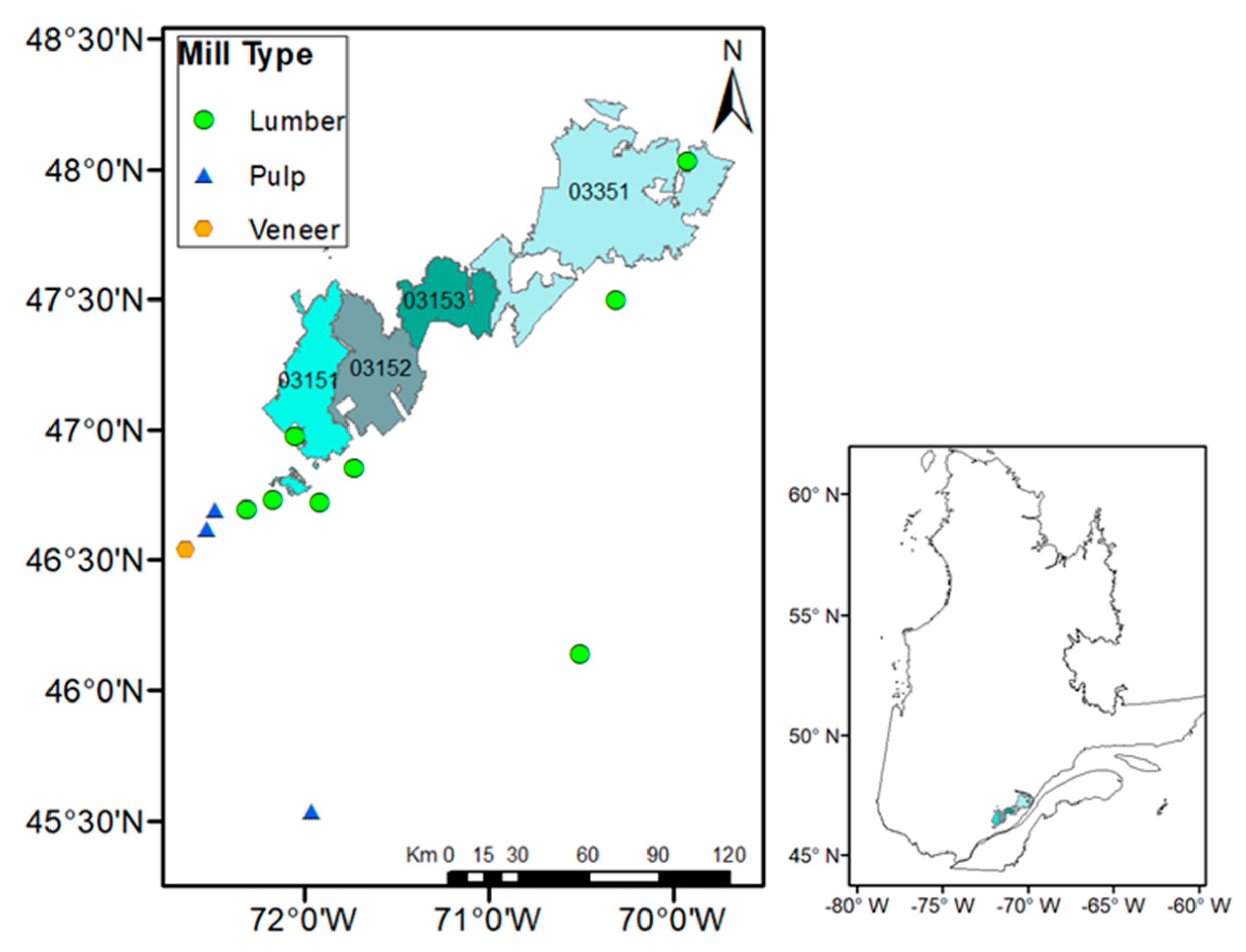
The models presented above were applied to a Canadian case study of public forests managed for timber production in the province of Quebec. We selected the forest region “Capitale Nationale,” which is an area that contributes significantly to the provincial economy through its forest industry. There are four forest management units (FMUs), namely, 031–51, 031–52, 031–53, and 033–51, in this region. The region is located between 69°30′ W and 73°30′ W longitude and 46°30′ N and 48°20′ N (Figure 1). Eleven wood mills have received timber license agreements for the planning period 2018–2023 in the region [40]. The mills manufacture various types of products using timber procured from the forests.

The case study region falls in the boreal bioclimatic domain of the northern temperate zone [42]. Of the total (gross) spatial area of 1.1 million ha, 53% is considered commercially productive public forest for timber production and can be made available for harvest (Table 1). In addition, 11% of the gross area was forested but not available for harvesting because it was covered by low productivity stands (stands that never yield more than 50 m³ha⁻¹ in their life spans) and excluded from AAC calculation. The rest includes private forests and water bodies (8%) and area reserved for biodiversity conservation (28%) [9]. Fifty-eight percent of the productive forest area is composed of softwood-dominating and the remaining 42% is hardwood-dominating stands. However, the percentage of the softwood and hardwood species dominance varies between 41% and 88% and 12% and 59%, respectively, in the four FMUs (

Table 2. Spatial information and status of standing volumes in the case study forests (four forest management units (FMU)).

FMU	Total (Gross) Area (ha)	Productive Forest Area (ha)	Standing Volume Total (m3)		Predetermined AAC+ (m3yr−1)
			Total	% Softwood	Hardwood	Softwood
FMU 031–51	174,990	112,771	12,282,565	41	71,800	65,300
FMU 031–52	172,650	113,620	8,273,231	63	27,800	61,900
FMU 031–53	216,010	84,403	4,728,352	88	6,300	50,400
FMU 033–51	521,080	264,440	17,781,000	59	97,000	138,600
Total	1,084,730	575,234	43,065,149	58	202,900	316,200

⁺ The upper limit of total AAC is 521,200 m³ according to BFEC model simulation (MFFP 2018).

).

The region is comprised of various forest cover types, such as pure hardwood (H), pure softwood (S), mixed hardwood (HH), hardwood-dominating mixed stands with softwood (HS), mixed softwood (SS), and softwood-dominating mixed stands with hardwoods (SH) (Figure 2a). Commercially, the important timber-producing hardwood species are yellow birch (Betula alleghaniensis), paper birch (Betula papyrifera), aspen (Populus grandidentata), sugar maple (Acer saccharum), Balsam poplar (Populus balsamifera), and red maple (Acer rubrum). Likewise, commercially important softwood species in the region are black spruce (Picea mariana), balsam fir (Abies balsamea), white spruce (Picea glauca), red spruce (Picea rubens), white pine (Pinus strobus), red pine (Pinus resinosa), and thuya (Thuja occidentalis). Individual trees with a diameter at breast height (DBH) above 9 cm and top diameter above 7 cm are considered timber-producing logs for both hardwood and softwood species [43] and were considered in this study. In terms of age structure, a majority of the stands are young (< = 50 years), and 40% are immature (> 50 and < = 75 years) (Figure 2b). The stands maturity classes are classified based on Jetté, et al. [44] for the forests in Quebec. The minimum harvesting age, which is defined as the age of the forest stand when it attains a minimum of 50 m³/ha of timber volume for the first time, varies between 50 and 75 years depending on the strata-specific growth rate.

The Bureau du forestier en chef [9] determines the AAC based on sustainable yield principle over a long-term (150 years) planning horizon divided into 30 5-year periods. Subsequently, timber license agreements are made with mills guaranteeing a specified amount of timber volume. The AAC determination by BFEC (Table 2) does not specify details regarding timber quality. Yet, information on timber quality is important, because mills require timber of certain specifications to produce a specific product. As an example, timber suitable for pulp production will not meet the quality requirements for manufacturing veneer or lumber. Eleven TLA wood mills process timber to produce five types of products, namely hardwood veneer (850 m³), hardwood lumber (58,000 m³), hardwood pulp (132,000 m³), softwood lumber (221,600 m³), and softwood pulp (39,150 m³). The values in parentheses represent the timber volumes allocated per year towards the product for planning period 2018–2023 [34].

Most of the forest stands in the study area are mixed stands of hardwood and softwood. It is mandatory for mills to harvest the entire cutblock that is assigned to them whether or not the timber meets the mill’s product specifications. For example, if a mill that only accepts hardwood is allocated a cutblock containing 70% hardwood and 30% softwood, it has to harvest both hardwood and softwood. As such, all timber harvested counts towards the AAC limit (Table 2).

2.3.2. Model Parameters

2.3.2.1. Stratification

Each of the forest management units is spatially stratified into geographically explicit regions, termed as “tarification zone,” that specifies costs based on distances between mills and the zone. Each of the zones was divided into strata based on ecodistrict (a contiguous spatial area characterized by relatively homogenous relief, geology, landforms, soils, vegetation, land use, etc. [45]), cover type (hardwood, softwood, and mixed wood), species dominance, and management practice (clear-cut and partial cut). We used stratum-based yield tables in order to address the variability of forest productivity by geographic and bioclimatic variations. In our simulation models, there were 243 strata altogether in four forest managements units, and the mean and median of the strata spatial size were 2368 ha and 1058 ha, respectively, ranging between 28 ha and 24,250 ha. Each stratum was a mixture of uneven-aged stands. The initial area of each stratum was kept in the 5-year age class interval from age class 1 (0–5 years) to 30 (145–150 years). According to this classification, there were 702 stands (substrata) altogether within the 243 strata at the start of our simulation. Adopting the Model III network structure [4,5], each stratum can contain up to 30 age classes, leading to a maximum of 7290 stands in total while simulating for 30 periodic plans. Volume tables and diameter class for each species are based on these age classes.

2.3.2.2. Forest Product Data

For each stratum, spatial data on stand areas, initial stand conditions, and yield tables of timber for the planning period 2018–2023 were accessed from MFFP [9]. Volume tables and quadratic mean diameter (qmd) by species for each age class interval were used in our simulation. Product recovery from timber varies depending on its allometric attributes such as diameter, length, and form factor. BMMB has developed and maintained a product recovery database for a number of commercial tree species by 2-centimeter DBH class that can be downloaded from BMMB [46]. For our simulation, this DBH classification (qmd for each age class) was used to transform timber volumes into primary processed products, namely veneer, lumber, and pulp, as required by the TLA wood mills.

2.3.2.3. Economic Parameters

The costs in the model simulation included expenses incurred for forest management, road construction and maintenance, harvesting, felling, forwarding, transportation, and product transformation. Selling prices represent the prices of the aforementioned five products. There are four grades of hardwood lumber and the proportion recoverable of each grade depends on the timber diameter class. Each grade of lumber has a different cost and price. Supply chain costs and product (veneer, lumber and pulp) prices for each stratum were obtained from [47]. Following BFEC’s manual, we used a discount rate of 4% yr⁻¹ for the first 30 years and 1% yr⁻¹ afterward [9].

2.3.2.4. Model Formulation

The LP models for a 150-year planning horizon by 5-year periods as done in MFFPQ [9] were simulated. It consisted of 30 planning periods (T) and 30 age classes (A). Our Model A (Equations (1)–(8)) is the reproduction of BFEC’s Woodstock model. Woodstock models can be downloaded from FTP (File Transfer Protocol) [48]. This reproduction allowed us to analyze the economic performance of the model prescriptions by locating the spatially explicit age classes of each harvest volume. It also helped validate our models by comparing our results with the BFEC’s AAC (timber volume) for the period 2018–2023 [40]. Following the current practices, Models A and B were optimized for an entire planning horizon. However, Model C was optimized only for the first 5-year period so as to synchronize the planning cycle of TLA. It was also simulated in a rolling planning horizon and the model outputs were stored for the 150-year planning horizon as in Models A and B.

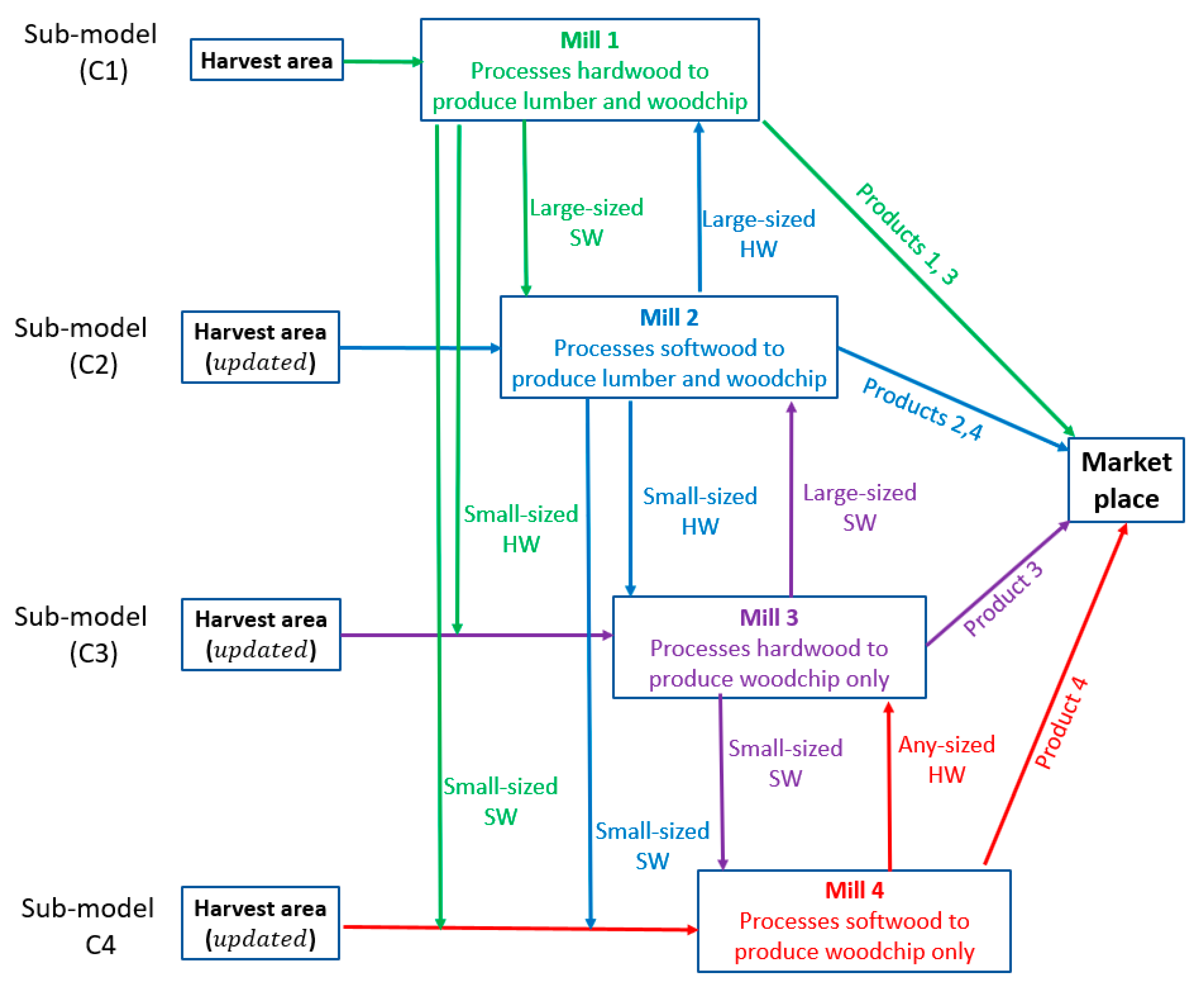
Of the five products manufactured by the TLA mills, we did not consider veneer in our Model C due to the very low volume (timber volume less than 1000 m³) committed in the TLA in the study area. We categorized the 11 mills that have TLA into 4 according to the types of product they manufacture. The mills grouped into categories 1 to 4 produce a) hardwood lumber, b) softwood lumber, c) hardwood pulp, and d) softwood pulp, respectively. Corresponding to these 4 products, 4 sub-models (C1–C4; Figure 3) were developed that maximized each product sequentially. The order of Mills from 1 to 4 (Figure 3) is based on the demand for and economic value of the products; the higher the order, the greater its economic importance. In addition, timber harvest for lumber can be transformed to woodchips, but timber harvest for woodchips cannot be sent to produce lumber. In the case study, only 4% of forest contained pure hardwood stands (Figure 2). The vast majority of hardwoods were present in mixedwood stands with softwood. The age at which the economic value is maximized is shorter for softwoods than for hardwoods. The timber specification for minimum DBH required to produce hardwood lumber is 24 cm, whereas that for softwood is only 14 cm [34]. Therefore, hardwood takes much longer time than softwood to reach its maximum potential value based on the yield curve [9] and value recovery [34]. If softwood is allocated first, all hardwoods in the cutblock are also harvested without allowing them to reach their maximum potential value for lumber production. Therefore, we set the model to fulfil the demand for hardwood lumber mills first. The simulation process is explained in detail in Figure 3 and Box 2.

Box 2. Steps of the simulation process for Model C (sequential optimization).

1.1.

In sub-model C1, the model maximizes the net present value of Mill 1 for the first planning period. Mill 1 processes large-sized hardwood timber to produce high-value lumber and wood chips. An even-flow constraint ensures sustained supply of high-value product over the planning horizon.

1.2.

For the mixed species cutblock, Mill 1 must harvest the entire cutblock including softwood. After harvest, hardwood timber is processed in Mill 1. Timber not used by Mill 1 is sent to other mills depending on its species and size, as depicted in Figure 3. Softwood volumes harvested are also counted towards the softwood annual allowable cut limit.

1.3.

The forest inventory is updated by deducting the areas harvested in step 1.1. Similarly, the AACs are updated for hardwood and softwood. Execution of sub-model C1 is complete.

2.

In sub-model C2, steps 1.1–1.3 are repeated for Mill 2. However, Mill 2 processes large-sized softwood timber to produce high-value lumber and wood chips. Execution of sub-model C2 is complete at this point.

3.

In sub-model C3, steps 1.1–1.3 are repeated for Mill 3. Mill 3 processes all hardwood timber into wood chips but does not send hardwood timber to Mill 1, because it has already met demand or would not get profitable supply. Execution of sub-model C3 is complete at this point.

4.

In sub-model C4, steps 1.1–1.3 are repeated for Mill 4. Mill 4 processes all softwood to produce woodchips. Execution of sub-model C4 is complete at this point.

5.

The next periodic (5-year) replanning is executed and steps 1–4 are repeated until the end of the planning horizon.

Prior to executing the model, an equation was adjusted to ensure that sub-model C1 (maximize NPV from hardwood lumber) would not consume all hardwood volumes outlined in AAC. If hardwood AAC is fulfilled by sub-model C1, the subsequent sub-model C2 (that targets softwoods) will not be able to harvest any of the mixedwood stands. To resolve this issue, a preliminary assessment was conducted to find the appropriate proportion to reduce the hardwood AAC in sub-model C1 so that the total revenue from all products would be maximum. The experiment consisted of the reduction of hardwood volume by proportion of 0.50, 0.40, 0.30, 0.20, and 0.10 from the optimal solution. Model optimization with a reduction by 20% (i.e., 80% retention) yielded the maximum net revenue for the entire sub-models (Models C1, C2, and C3) that were embedded into Model C. Therefore, hardwood AAC was reduced by 20% in sub-model C1 through adding a parameter in Equation (13), the modified version is shown in Equation (20). This reduction with this heuristic approach provided enough hardwood for sub-model C1, while still allowing mixedwood stands to be harvested in sub-model C2 (maximized NPV from softwood lumber). It resulted in the maximum possible net profit for the entire supply chain.

$${{\displaystyle \sum }}_{s\in S}{{\displaystyle \sum }}_{g\in M_i}{{\displaystyle \sum }}_{a\in A}{h}_{sa1\_M_1}\left(v_{s{a}_g}\right)\le AA{C}_{g\in G}\left(0.80\right)$$

(20)

These LP models were solved using mathematical modeling language AMPL [46] and Gurobi 5.6.0 solver (Gurobi Optimization Inc., Houston, TX).

The model-prescribed solutions in Models A and B are the harvest areas by stratum and age class for the 5-year planning periods ($h_{sat}$). Model C also prescribes the harvest area but in such a way that the area gives the most possible timber volume of desired species that is usable and most profitable for the specified Mill ($h_{sa1\_M_i})$ (Figure 3). The periodic harvest attributes (area, volume, net revenue) were annualized by dividing the model solutions by 5 because of the 5-year planning period and reported the results in terms of value ($) and harvest volume (m³) in annual base. The LP solutions were analyzed using statistical programming software R [49].

3. Results

3.1. Initial State of Merchantable Timber Volume

At the start of our model simulations, the total merchantable volume (standing timber of DBH ≥ 9.1 cm) in the study area was estimated to be 43 Mm³ (75 m³ha⁻¹) with softwood contributing 58% (Table 2). Seven percent of the hardwood volumes had veneer- and lumber-producing quality (DBH ≥ 24 cm) and 87% of softwood had lumber-producing quality (DBH≥14 cm). At the end of the planning horizon, the estimated total growing stocks after the 30th period using Models A and C were 48 Mm³ (hardwood 16 Mm3, and softwood 32 Mm3) and 45.5 Mm³ (hardwood 15.5 Mm³, and softwood 30 Mm³), respectively.

3.2. Timber Flow Using Models A, B and C

As expected, Model A produced the same amount of total harvest volume as the AAC (the capped amount) (Table 2 and

Table 3. Product-wise timber license agreement (TLA) volumes, model-simulated harvest volumes, and net revenue generated using three models, assuming that all the prescribed volumes are harvested but sold under two distinct scenarios: a) all the harvested volumes regardless of negative net revenue for any product, and b) only the volumes that produce positive net revenue by product for the first period.

		TLA (m3yr−1)	All Harvests are Supposed to Be Sold			Harvested Stands Producing Only Positive Net Revenue are Sold
			Model A	Model B	Model C	Model A	Model B	Model C
Harvest Volume (m−3 yr−1)	Total volume	451,750	521,200	521,200	521,200	302,559	347,051	502,240
	Lumber	280,800	312,135	372,707	380,775	151,183	234,801	363,995
	Pulp	170,950	190,207	110,301	98,909	136,084	77,105	97,500
	Hardwood	155,700	188,282	168,948	165,624	146,072	134,453	162,916
	Lumber	59,200	11,576	58,647	66,715	9,987	57,348	65,416
	Pulp	96,500	176,706	110,301	98,909	136,084	77,105	97,500
	Softwood	296,050	314,060	314,060	314,060	141,195	177,454	298,579
	Lumber	221,600	300,559	314,060	314,060	141,195	177,454	298,579
	Pulp	74,450	13,501	0	0	0	0	0
	Harvest area (ha)		4277	3679	3794	2198	2238	3524
	Harvest area (%)		0.74	0.64	0.65	0.38	0.39	0.61
Net Revenue ($ yr−1)	Total net revenue		10,499,909	14,314,454	15,327,485	5,429,509	9,196,482	14,177,106
	Hardwood total		1,330,247	2,991,410	3,528,270	1,587,601	3,161,171	3,541,536
	Veneer		3367	17,916	0	2903	17,590	0
	Lumber		512,278	2,509,928	2,991,795	441,123	2,494,520	2,975,172
	Pulp		814,601	463,566	536,476	1,143,574	649,061	566,364
	Softwood total		9,169,661	11,323,048	11,797,883	3,841,909	6,035,313	10,633,531
	Lumber		4,293,514	7,077,819	7,374,232	2,011,828	3,936,718	6,462,414
	Pulpwood		4,876,147	4,245,230	4,423,651	1,830,081	2,098,595	4,171,117

). We further disaggregated the total timber disbursement to each wood mill category corresponding to each product type based on the product recovery proportion (hardwood and softwood sawlog, pulplog). In many strata, the net revenue generated by the harvest prescriptions using Model A was negative for some products (e.g., hardwood pulp). If it were assumed that the stands that generated negative net revenue from at least one product (we intended to reduce unprofitable losses) were not harvested, the total volume of hardwood harvested would have been 146,072 m³yr⁻¹. This is 6% below the current TLA volume. Likewise, the reduction of softwood timber would have been 48% below the TLA in the first period (Table 3). The differences were more prominent for the high-value (lumber) timber lowering the total net revenue by 52% and 42% for hardwood and softwood, respectively (Table 3). Such discrepancy between these two scenarios (with or without considering product wise net revenue) can be observed throughout the planning horizon (Figure 4a,b).

Changing the objective function of the optimization model to maximize the global NPV for the supply chain led to different outcomes, particularly for hardwood lumber production (Figure 4c). Within the limit of AAC, Model B prescribed more large-sized hardwood timber (58,647 m³yr⁻¹ compared to 11,576 m³yr⁻¹ using Model A), reducing pulpwood volume in the first period. The pulpwood supplies surpassed the TLA requirement by far, but hardwood timber for lumber production was still in short supply (Table 3). This model prescribed non-declining flow of large-sized timber (sawlog) over the planning horizon, except in a few earlier periods (Figure 4c). In contrast, Model A produced volumes well below the TLA level and fluctuated substantially over the planning horizon (Figure 4a). Model B produced 314,060 m³yr⁻¹, which came from all the large-sized timber and remained above the current total TLA level (296,050 m³yr⁻¹) (Table 3). It did not schedule harvesting of small-sized timber even for pulpwood (Table 3). Although the gap between high-value TLA volume and AAC is decreasing over time using Model B (Figure 4c), there is still a big gap over the profitable harvest volume and AAC over the planning horizon (Figure 4d).

Using Model B, a significant loss in net revenue (from softwood) was observed under the scenario which avoided harvest of stands with products that generated negative net revenue (Table 3). Model C attempted to lessen such losses by executing sub-models that sequentially maximized NPV for each mill (product type), starting from the highest-value lumber mill to the lowest-value pulp mill. This formulation ensured that current TLA requirements are met by harvesting stands that would produce only positive net revenue. Using Model C, the total harvest volume was 96% of AAC when stands containing products with negative net revenue were not harvested. This is a significant improvement from Model A (58%) and Model B (68%). The difference of harvest flows between the two scenarios were very subtle in Model C (Figure 4e,f) as compared to Models A and B. The gap between the profitable high-value TLA volume supply and predetermined AAC is gradually decreasing over the planning horizon (Figure 4f). In this regard, Model C seems superior to Models A and B.

3.3. Economic Performance Using Models A, B and C

The economic performance of harvest prescriptions made by Model A was assessed. Assuming that all the harvested timber was processed and sold in the market, the estimated revenue was $10.5 million ($18.25 ha⁻¹) yr⁻¹, in which softwood contributed 87% ($9.2 million yr⁻¹) (Table 3). The net revenue per unit of softwood and hardwood harvest volumes were $29.20 m⁻³ and $6.42 m⁻³, respectively. The total net revenue (sum of hardwood and softwood) per unit of harvest area was estimated to be $2455 ha⁻¹. As in the case of harvest volume, the difference in total revenue generated using Model A between the two scenarios were very high over the planning horizon. The differences were higher in the net revenues generated by softwood products than that generated by hardwood products (Figure 5a,b).

Furthermore, the economic performance of prescriptions obtained using Model B was evaluated. The estimated net revenue was $14.31 million yr⁻¹ ($24.87 ha⁻¹yr⁻¹), assuming that all harvested timber was processed and sold. The net revenue obtained using Model B was substantially higher (+36%; Table 3) than Model A. In addition, Model B yielded non-declining net revenues from high-value (lumber wood) timber over the planning horizon, except in a few early periods (Figure 5c) as compared to Model A. The net revenue per unit of softwood and hardwood harvest volumes were $36.05 m⁻³ and $14.44 m⁻³, respectively. The net revenue per unit of harvest area was $3891 ha⁻¹ which is substantially higher than that using Model A ($2455 ha⁻¹).

The net revenue reduced by 64% when stands with negative net revenue products were not harvested in the first period (Table 3). This is still an improvement of 10% in comparison to the net revenue generated using Model A. The difference in revenues generated between the two scenarios existed throughout the planning horizon (Figure 5c,d). There was actually an increase in net revenue obtained from hardwood (5%) and a substantial reduction from softwood. The reduction in net revenue was observed throughout the planning horizon (Figure 5d). This is due to a reduction in the harvest of stands with small-sized hardwood which also contain large-sized softwood (Figure 4d) that were left unharvested. As a result, Model B could not fulfil the current TLA requirements, although there was an increase in the harvest of large-sized hardwood timber (Figure 4d).

Model C produced slightly higher total net revenue than Model B under the assumption that all the products are sold in the market (Table 3). The net revenue per unit of softwood and hardwood were $37.57 m−3 and $17.04 m−3, respectively. Similarly, the net revenue per unit of harvest area was $4040 ha−1, which was substantially higher than Model A ($2455 ha−1) and Model B ($3890 ha−1). In contrast to Model B, Model C helped gain net revenue from large-sized harvest timber in the initial periods, while the net revenue from softwood (lumber and pulp) was not substantially different under the assumption that all the harvests were sold over the planning period (Figure 5c,e). However, under the scenario where stands containing negative net revenue products were not harvested, Model C prescribed higher volumes of softwood (Figure 4f), and hence generated higher net revenue in comparison to other models throughout the planning horizon (Figure 5f).

4. Discussion

Our estimates of standing merchantable timber (DBH greater than or equal to 9.1 cm) volume of 43 million m³ was close (44.5 million m³) to that estimated by BFEC (BFEC 2014). Moreover, our estimate of AAC of 521,200 m³yr⁻¹ (hardwood 207,140 m³yr⁻¹ and softwood 314,060 m³yr⁻¹) met the maximum ceiling set by the BFEC’s Woodstock models [9]. These comparisons served to validate our results (produced by our three models) with the existing estimates. Subsequently, supply chain economic performances of the three models were evaluated.

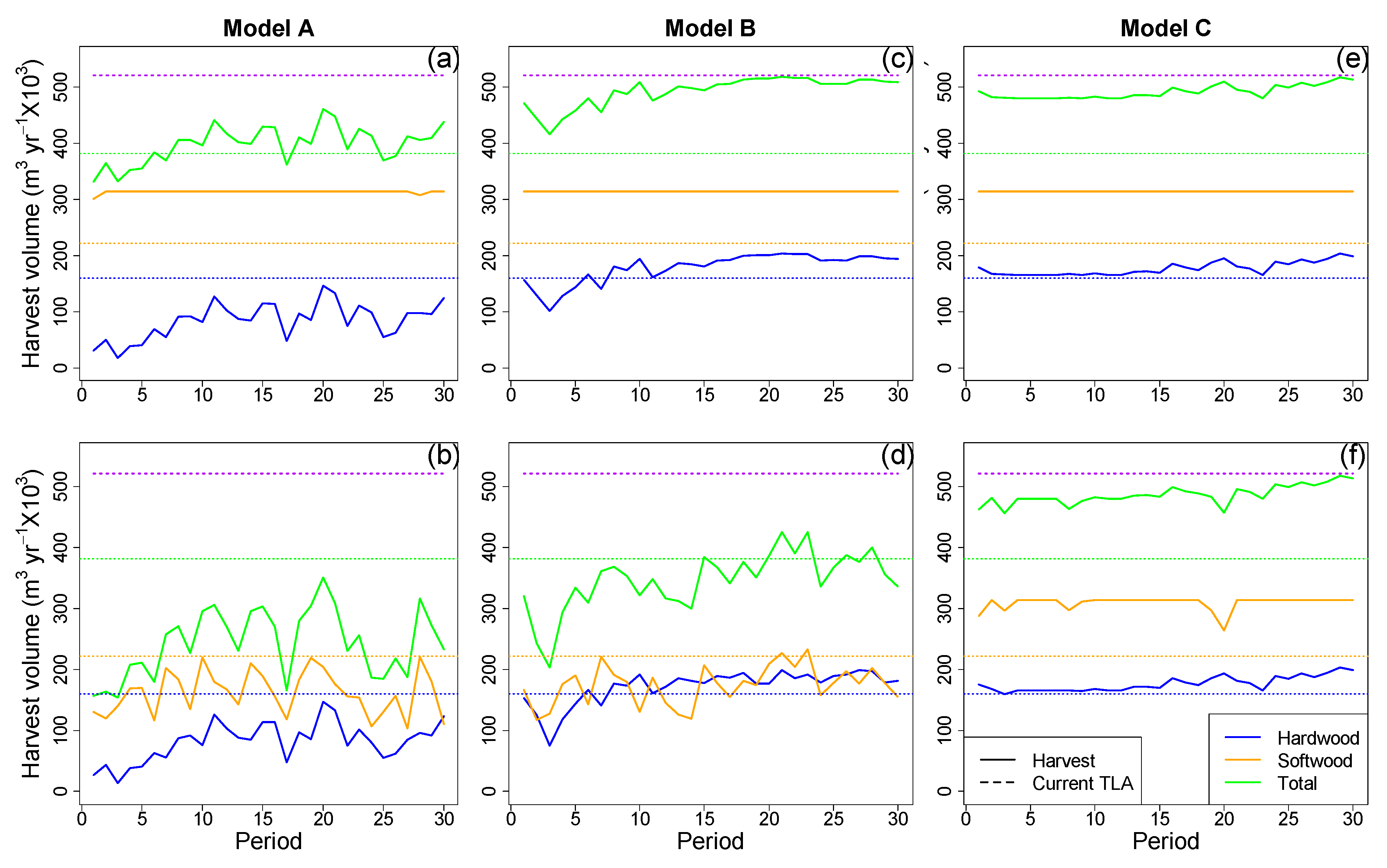
Even flow of harvest volume and non-declining growth over the planning horizon is used as an indicator of sustainable forest management. So, planning models are designed to generate an even flow of timber with or without inventory constraint at the end of the planning horizon. The even-flow constrained models simulated in a periodic replanning framework for a 150-year planning horizon protects non-declining growing stock for an even longer time period. Our results show that the growing stock at the end of the planning horizon was higher than the initial growing stock. While observing the product types recovered from harvested timber over the planning horizon by the business-as-usual harvest planning model (Model A), we found that there was a large fluctuation (Figure 4a) despite an even flow of total timber volume by period. In addition, there was product-wise discrepancy between the AAC and industrial timber allocations (TLA requirement). There was a short supply of high-value and over-supply of low-value timber, particularly of hardwoods. Timber-volume-based AAC calculation using Model A can create discrepancy between forest product supply and industrial demand. Approximately 20% of the AAC (30% hardwood and 10% softwood) in Canadian forests was not harvested in the past decade (2007–2017) [49]. This may partly be explained by the lack of integration between forest management and industrial demand [10]. Our study in mixed stands showed greater discrepancy; using Model A, 42% of the AAC could not be harvested profitably. Even in pure stands, only 81% hardwood and 95% softwood AAC could have been harvested profitably because of a higher proportion of low-value pulp wood.

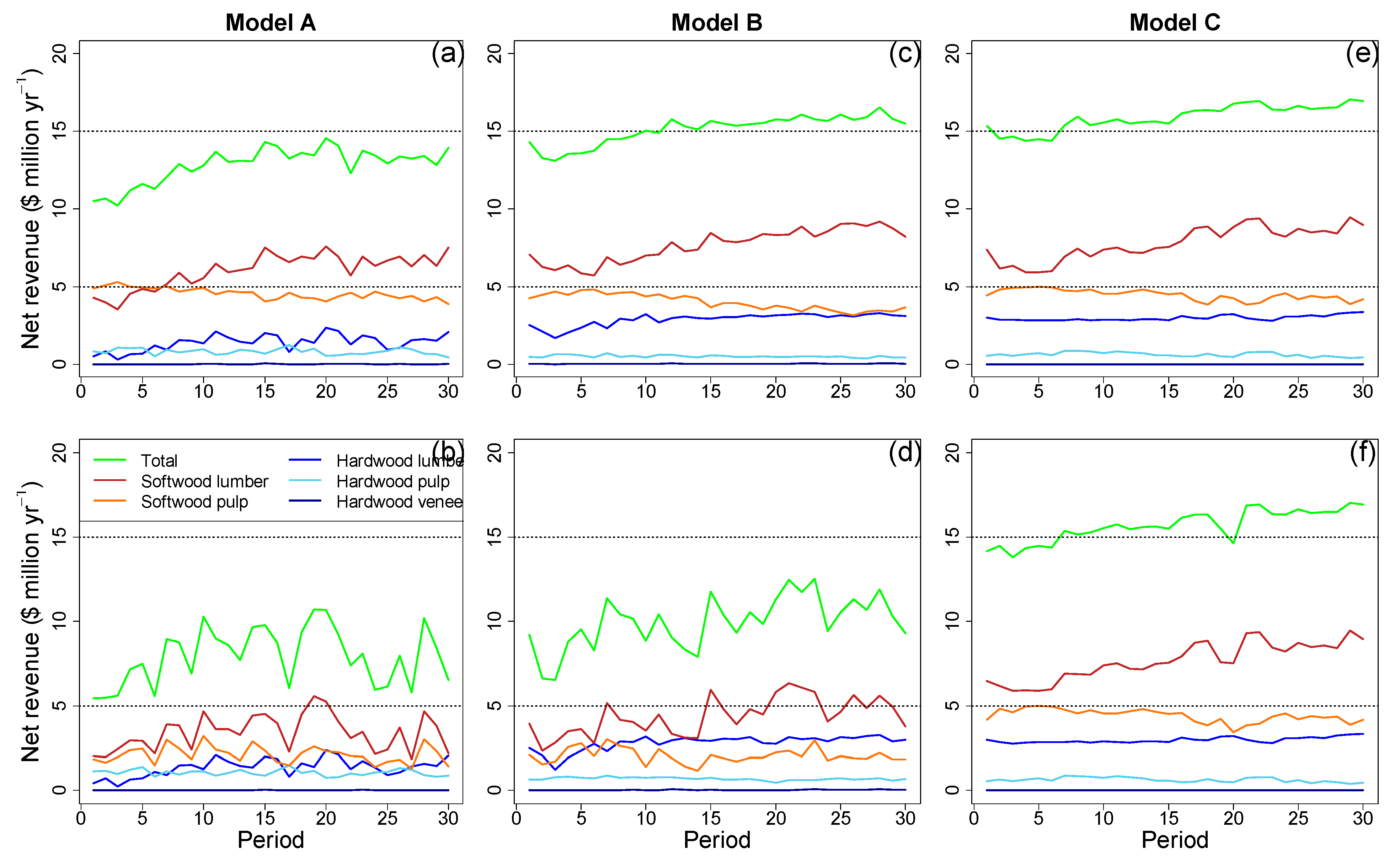
Our second model formulation (Model B) follows a vertically integrated policy that accounts for economic values. It maximizes the NPV of the supply chain network ensemble. Not surprisingly, this model was superior to Model A as it increased the net revenue by 33% for the first planning period (Table 3). Earlier, Bouchard et al. [30] showed that an integrated NPV maximization model increased the revenue by 13% compared to a nonintegrated NPV maximization model in a study carried out in the same forest management unit. The improvement in supply chain net revenue varies widely between volume-maximized and revenue-maximized models, and nonintegrated and integrated models, depending on the forest conditions [22]. However, it can still be observed the discrepancy between demand and profitable supply using such an integrated model while supplying to the TLA mills. Current forest management practice (e.g., Cutting with Protection of Regeneration and Soils (CPRS) in Quebec [38] is largely dominated by a clear-cut harvest system that requires harvest of all species or species groups in the cutblock. In order to favor one product supply to one specific TLA wood mill, another product supply may generate unprofitable (net) revenues. In our case study, Model B generated substantially high net revenue through the sale of softwood as long as it compensates for the losses of hardwood pulp. If we assess the individual wood mills’ benefit and cost, a substantial amount of harvest volumes cannot be used unless the mills run at a loss. If the stands that are producing negative net revenues are not harvested, TLA volume cannot be met (Figure 4). Our results corroborate the findings in Paradis et al. [36], who showed that, in order to reduce the discrepancy between demand for and supply of hardwood, softwood harvest was reduced by 32% (please refer to their Figure 8), potentially creating supply shortage for softwood mills.

In Models A and B, it was observed that avoiding harvest of stands with negative net revenue can lead to a lost opportunity, particularly in mixed stands (Table 3). In addition, the reduction of wood flow leads to losses in employment opportunities and regional economic activities [26,29,50]. Model C prescribed 96% of AAC, meeting TLA requirements with profitable supply. The higher net revenue generated using Model C can be attributed to harvests of more large-sized timber, increasing economic efficiency. Model C not only protects harvests of immature hardwood but also tends to reduce early harvest of softwood while maintaining sustained flow of large-sized timber over the planning horizon. According to the yield and product recovery curves that we used, the merchantable volume and lumber recovery proportion for softwood attain their maxima earlier than that for hardwood. Due to these growth behaviors, the net revenue for softwood mills did not decrease even though hardwood was given the priority through the first sub-model. Therefore, reverse sequencing, i.e., ordering our sub-models to prioritize softwood first, could create lower net revenue due to potential losses from hardwood (financially immature) harvest due to the inclusion of a suboptimal component. This phenomenon can partly explain why the global model (Model B) can often produce unprofitable prescriptions to all of the TLA mills, despite the superior total supply chain profit. Hence, Model C supported our hypothesis of value creation potential by increasing supply chain efficiency, while also fulfilling product-wise TLA requirements profitably. The strength and novelty of this approach, therefore, is to allow each mill to operate profitably and let the unprofitable stands grow and build more value for the subsequent periods.

As mentioned earlier, it is no surprise that Model C is superior to Model A because of the objective formulation that maximizes net revenue. Theoretically, global NPV maximization using Model B (global maxima) should be superior to Model C (product disaggregate) that solves for each product (local maxima). Model C generated higher net revenue than Model B for the first period (Table 3), which can be attributed to the fact that Model C maximized NPV only for the first period, whereas Model B maximized the NPV for the entire (30 periods) planning horizon. Model C further seems superior to Model B for all products’ profitable supply over the planning horizon (Figure 5f)). Two factors have led Model C to be superior to Model B in total net revenue generation in our particular case study. The first factor is that any stands that generate positive net revenue (from the sum of all products) are eligible for harvest in Model B. Model C attempts to avoid stands that would generate products with negative net revenue. This avoidance in the preceding periods can permit capital generation for the subsequent periods due to tree growth and subsequent value [41]. The year of postponement of harvest depends on the Models as presented by Rijal et al. [29,41]. Model B does not wait until the hardwood reaches full economic maturity due to immediate gain from softwood and an applied discount rate. Model C1, however, must wait until full maturity of hardwood. This mechanism can help make a stable supply of high-value products over the planning period. The second factor is that, if a particular supply of timber generates negative net revenue for high-value production, Model C formulation allows its re-evaluation by subsequent sub-models. For example, if a particular supply of large-sized hardwood timber is not profitable for Mill 1 to produce lumber (e.g., due to lower conversion factor and long transportation distance), the timber can be sent by subsequent sub-model to Mill 3 to produce pulp.

Model C has an ecological advantage compared to Models A and B. It uses residue from lumber production to fulfil the demand for pulpwood (Table 3). Consequently, pulp production from residual lumber wood was substantially higher using Model C than in Models A and B. It lowers immature harvest for pulp production. If demand for sawlog is met, that sub-model that maximizes pulpwood can draw from the available large-sized timber. Our model did not protect against such sacrifices as the objective was to fulfill the TLA volumes of each product-wise mill. Moreover, there is an opportunity to extend harvesting of a stand until timber attains sizes big enough to produce lumber in the subsequent planning period. As a result, Model C prescribed the lowest area to harvest. Reduction in harvest area not only implies the reduction in harvest and transportation costs but also permits robust forest planning in the face of forest disturbances [29,41,51]. Transportation cost contributes a significant portion in the total cost over the forest product supply chain. Selection of an optimal mode of transportation and uses of local biofuel can increase the financial efficiency while reducing the amount of carbon emission directly and indirectly [52]. However, consideration of such attributes was beyond the scope of our study. The substantial deferral of harvest by Model C leads to a higher proportion of old-growth forest [41], and hence more biodiversity integrity [53].

Our study was founded on the same set of assumptions for all three models to facilitate meaningful comparisons. The analysis assumed that the economic values of manufactured products would remain constant throughout the planning horizon. Our model relies on empirical data and it is very sensitive to any kind of value-attributing parameters such as product recovery factor, growth and yield table, product-wise costs, and prices. Moreover, different forests can be managed to produce a different set of products. Our method was applied to a case study with five product types, but it can be applied to other sets of products. The order of the sequential sub-models can be changed at the start of each periodic planning, depending on the supply chain objectives. Therefore, this modeling approach is flexible. The model can be useful to schedule harvesting when mutual negotiation is required among several mills attempting to procure wood from the same forest. This method promotes non-declining flow of high-value timber throughout the planning horizon, which is an important criterion of any wood industries to function for a longer period of time and provide a sustainable forest-based circular economy. This study entirely focused on the long-term demand for and supply of timber for product-specific industrial transformation and the search of potential alternatives to increase economic value of the timber flow within the predetermined AAC frame. Therefore, we did not consider other aspects of forest values besides timber supply economics. Nevertheless, sustainability of the wood industry is only possible if a forest ecosystem is sustainable. From this perspective, our work remained implicit in sustainability of diverse aspects of forestry resources and explicit in industrial sustainability. Furthermore, our model does not consider the potential risk of forest disturbances and market externalities. We used a static growth model, assuming that the growth and yield regime remains the same throughout the planning horizon. Future research can have extended avenues to include as many forest values in the forest supply chain, use of dynamic growth models, and adopt potential risks on forest values over the supply chain.

5. Conclusions

We formulated a novel modeling approach for long-term forest management planning that takes into consideration forest-product supply chain parameters. The output of the modeling approach was compared with the existing models using empirical data from commercially managed forests in the province of Quebec. The analyses results confirmed our hypothesis that our model can help increase the supply of high-value products and increase supply chain net revenues. A fundamental difference between our approach (Model C) and an integrated global model (Model B) is that the former sequentially allocates products starting with high-value-generating mills. The latter model attempts to maximize the global supply chain value, disregarding the benefit and cost of individual mills. Our model lowers the discrepancy between AAC and timber harvest. This procedure can be used in mixed-species as well as single-species stands. This model is flexible, but its application in any forest planning requires empirical supply chain data with region-specific parameters. The order or the number of the sub-models can be changed dynamically in response to market conditions. In addition, it protects against harvesting of stands that generate negative revenue. Instead, harvesting is delayed until all products can generate positive revenues, resulting in increased circular economic efficiency by generating higher net revenue per unit of harvest area and volume. Our modeling framework did not account for sources of externalities such as changes in market, production regimes, and impact of disturbances. Nevertheless, the modeling structure provides flexibility to accommodate such changes.