Improved Representation of Flow and Water Quality in a North-Eastern German Lowland Catchment by Combining Low-Frequency Monitored Data with Hydrological Modelling

Abstract

Achievements of good chemical and ecological status of groundwater (GW) and surface water (SW) bodies are currently challenged mainly due to poor identification and quantification of pollution sources. A high spatio-temporal hydrological and water quality monitoring of SW and GW bodies is the basis for a reliable assessment of water quality in a catchment. However, high spatio-temporal hydrological and water quality monitoring is expensive, laborious, and hard to accomplish. This study uses spatio-temporally low resolved monitored water quality and river discharge data in combination with integrated hydrological modelling to estimate the governing pollution pathways and identify potential transformation processes. A key task at the regarded lowland river Augraben is (i) to understand the SW and GW interactions by estimating representative GW zones (GWZ) based on simulated GW flow directions and GW quality monitoring stations, (ii) to quantify GW flows to the Augraben River and its tributaries, and (iii) to simulate SW discharges at ungauged locations. Based on simulated GW flows and SW discharges, NO₃-N, NO₂-N, NH₄-N, and P loads are calculated from each defined SW tributary outlet (SWTO) and respective GWZ by using low-frequency monitored SW and GW quality data. The magnitudes of NO₃-N transformations and plant uptake rates are accessed by estimating a NO₃-N balance at the catchment outlet. Based on sensitivity analysis results, Manning’s roughness, saturated hydraulic conductivity, and boundary conditions are mainly used for calibration. The water balance results show that 60–65% of total precipitation is lost via evapotranspiration (ET). A total of 85–95% of SW discharge in Augraben River and its tributaries is fed by GW via base flow. SW NO₃-N loads are mainly dependent on GW flows and GW quality. Estimated SW NO₃-N loads at SWTO_Ivenack and SWTO_Lindenberg show that these tributaries are heavily polluted and contribute mainly to the total SW NO₃-N loads at Augraben River catchment outlet (SWO_Gehmkow). SWTO_Hasseldorf contributes least to the total SW NO₃-N loads. SW quality of Augraben River catchment lies, on average, in the category of heavily polluted river with a maximum NO₃-N load of 650 kg/d in 2017. Estimated GW loads in GWZ_Ivenack have contributed approximately 96% of the total GW loads and require maximum water quality improvement efforts to reduce high NO₃-N levels. By focusing on the impacts of NO₃-N reduction measures and best agricultural practices, further studies can enhance the better agricultural and water quality management in the study area.

1. Introduction

Lowland catchments are characterized by a high groundwater (GW) table, low flow velocity, flat topography, and a significant presence of organic soils [1,2,3,4]. In the past centuries, different anthropogenic activities, such as river regulations, enhanced groundwater abstraction, and provision of artificial drainage to ensure better agricultural activities, have caused an impact on ecology, water balance, and nutrient dynamics, resulting in eutrophication and water quality deterioration [5,6]. Diffuse pollution from agriculture has increased considerably over the past few decades due to human activities related to the surplus use of both organic and synthetic fertilizers [7,8]. Over application of nitrogen (N) fertilizers to the crops in thin soils with steeper terrain causes significant damages to the environmental ecosystem, especially during the wet seasons [9]. Surplus nitrogen input is identified as a key contributor to the increased nutrient concentrations in the surface, ground, and coastal waters [10].

In Europe, agricultural activities continue to affect the surface water (SW) and GW quality in terms of NO₃-N pollution [11,12,13]. The EU nitrate directive was introduced in 1991 to identify and reduce the NO₃-N pollution in water bodies (Directive 91/676/EEC), and it focuses on integrated management of water in river catchments to acquire, improve, or maintain a good chemical and ecological status. Despite enormous efforts, a large ratio of European GW and SW bodies still do not comply with the “good chemical and ecological status” according to the defined criteria of the European water framework directive (EU-WFD). One reason is the still-poor identification, quantification, and management of diffuse pollution sources. The EU-WFD demands to reach a good chemical and ecological status of freshwater bodies by the year 2027. In the case of Germany, improvements are required due to the possible surplus use of agricultural fertilizers. Germany is continuously struggling with GW NO₃-N concentrations higher than 11.3 mg/L, a threshold for a “good chemical and ecological status” of GW [14,15]. Due to deficiencies in implementing the ordinance of agriculture fertilizer application and surplus use of both synthetic and organic fertilizers, a rise in NO₃-N concentrations in comparison to the reported NO₃-N concentrations from 2004 to 2007 is observed [16,17]. In 2016, the European court of justice brought legal action against Germany due to deficiencies in implementing the ordinance of agriculture fertilizer applications [7,18].

The whole situation stresses the more effective measures needed to understand and reduce diffuse NO₃-N emissions, transport, and transformation processes, especially for lowlands with intensive agricultural activities. This demands high spatio-temporal hydrological and water quality monitoring at a catchment and regional scale. Normally, high-resolution monitoring data in most of the lowland catchments are not available to reliably quantify and access the chemical and ecological status of water bodies and to identify critical areas and/or hidden point sources requiring the maximum measures to reduce the SW and GW NO₃-N concentrations. A detailed water and mass balance information is essential to develop and improve the management practices of water resources, as SW and GW interactions mainly control the NO₃-N dynamics in lowland rivers [19]. Physically based hydrological models can quantify the GW and SW interactions, and can simulate GW flow directions and SW discharges at ungauged locations. Hydrological modelling results, in combination with low-frequency monitored water quality data, can estimate the SW and GW NO₃-N pollution loads at catchment and sub-catchment scales. To select a suitable modelling tool to simulate Augraben catchment (a typical representative of north-eastern Germany lowland catchments), four different process-based models, “SWAT” (soil and water assessment tool), “SWIM” (soil and water integrated model), “HSPF” (hydrological simulation program—FORTRAN), and a coupled “MIKE SHE and MIKE 11” model, are reviewed. These models are compared by concentrating primarily on temperate-climate lowland catchments with intensive agricultural land use. Appendix A shows the summary of reviewed models based on simulated hydrological and hydraulic processes, governing equations, input data requirements, spatial and temporal discretization, and limitations [20,21,22,23,24,25,26,27,28,29,30,31]. The physically based distributed coupled MIKE SHE and MIKE 11 model is selected in this study to quantify the detailed water balance, simulation of surface flows at ungauged locations, and interactions of GW and SW at a desired level of complexity.

This study uses available low-frequency monitored flow and water quality data in combination with integrated hydrological and hydraulic modelling to represent the SW and GW hydrology and NO₃-N loads in Augraben River catchment. The research objectives of the present study include: (i) Detailed water balance estimation and quantification of GW and SW interactions, (ii) application of simulated SW discharges at ungauged locations to calculate NO₃-N loads at each SW tributary outlet (SWTO), (iii) estimation of the saturated zone represented by each GW quality monitoring station and quantification of GW contribution to the SW NO₃-N loads, (iv) identification of critical areas and sources mainly contributing to the water quality deterioration, and (v) estimation of a nutrient balance at Augraben River catchment outlet to evaluate the magnitude of NO₃-N transformations and plant uptakes.

2. Material and Methods

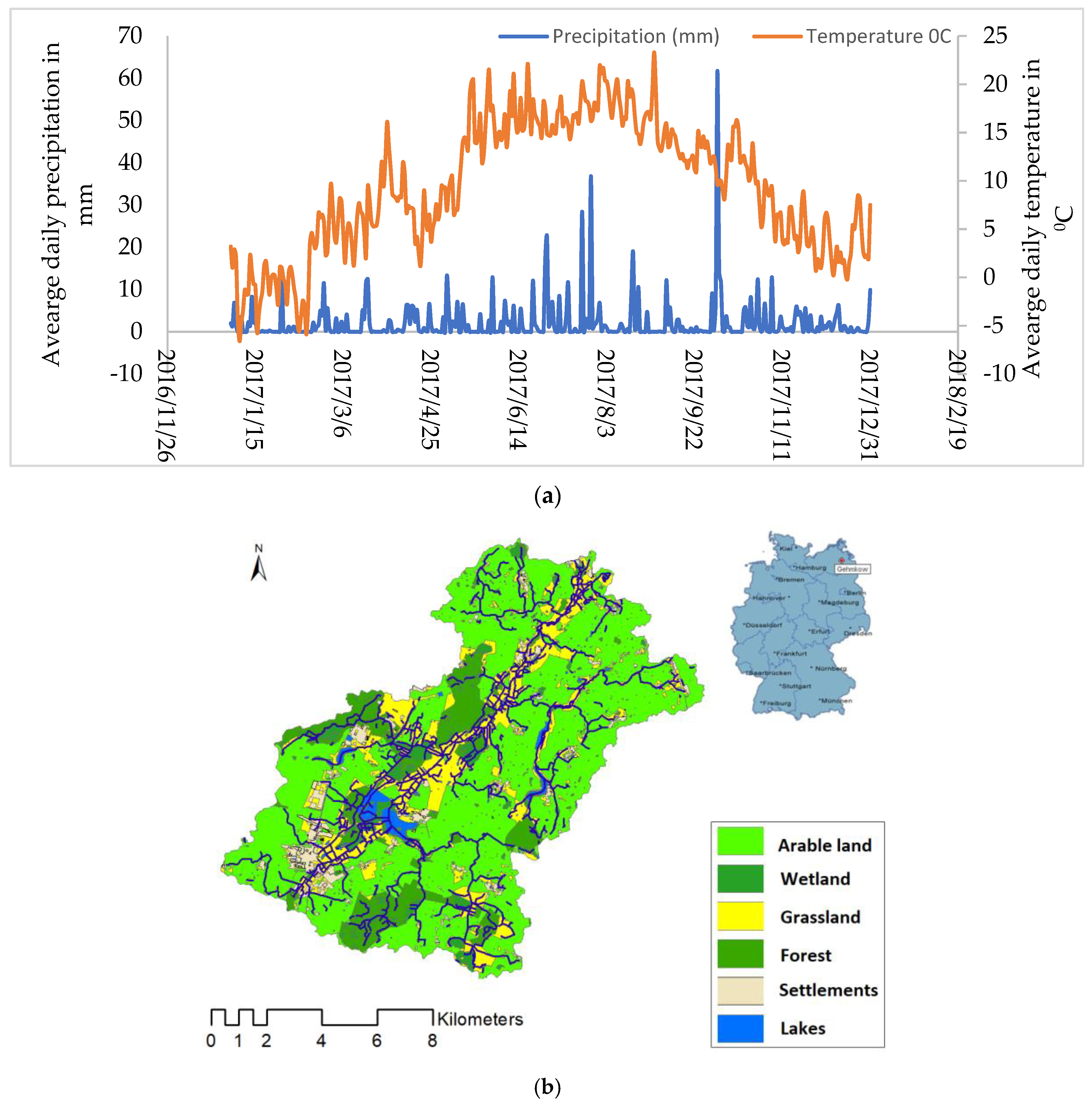
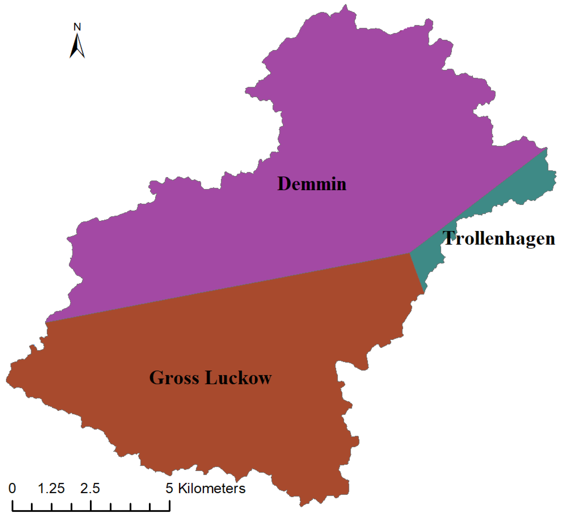
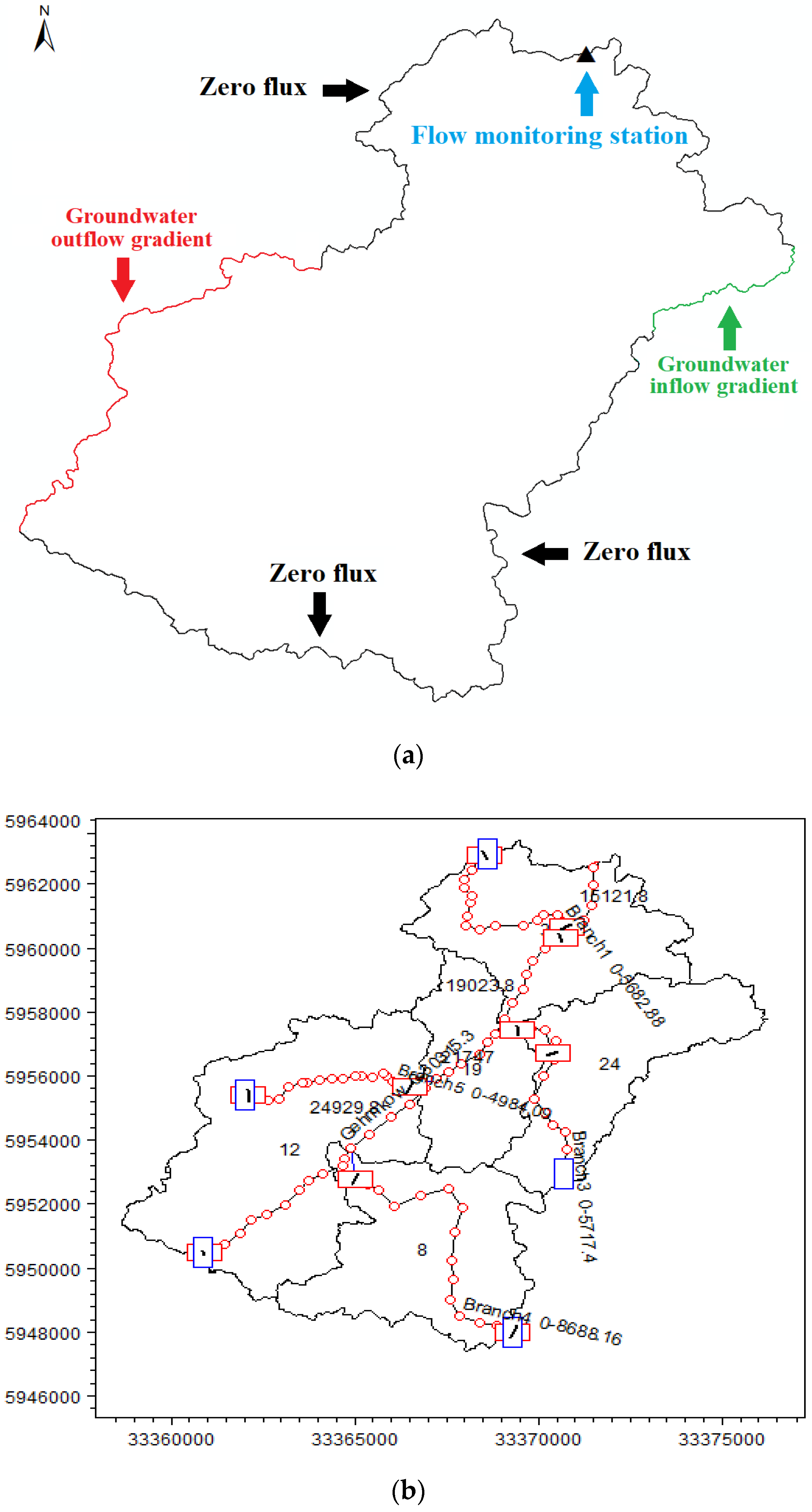
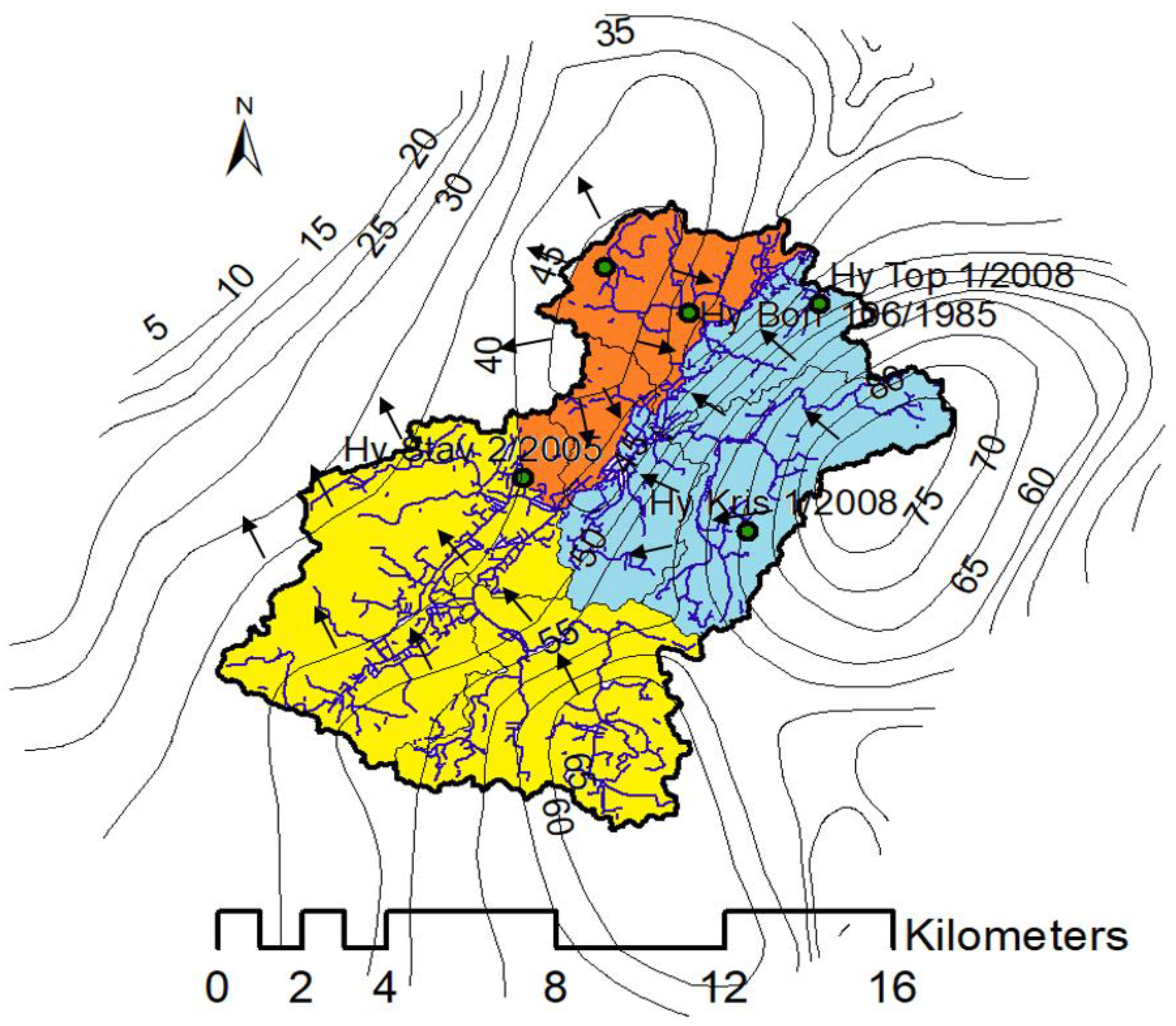
2.1. Study Area

Augraben River is the largest tributary of the Tollense River in terms of discharge and length. It is located in the lowlands of north-eastern Germany and is representative for the typical lowland flood plains of Central Europe. The Augraben River has a total length of 18 km up to the gauge station Gehmkow. The area of the Augraben River catchment up to the gauge station Gehmkow is 90 km². In the study area, the precipitation normally happens throughout the year in Augraben River catchment, with the most precipitation during the 31 days centred around July. The least precipitation normally occurs around February. On average, the temperature normally varies from −1 to 25 °C, and is rarely below −8 °C or above 31 °C during the course of the year. The wet season lasts from May to February, with more than 24% chance of a given day being a wet day. The drier season lasts from February to May (https://weatherspark.com/ and https://dwd.de). Figure 1a shows the average monthly temperature and precipitation in the study area during 2017. The topography is very flat in the study area. The lowest points at the Augraben River bed level vary between 40 (u/s) and 28 m (d/s) above NN (Reference Level).

The main tributaries of Augraben River include Lindenberg, Hasseldorf, and Au II Kentzlin. Three wastewater treatment plants (WWTPs) are located within the Augraben River catchment: WWTP_Lindenburg, WWTP_Ivenack, and WWTP_Stavenhagen. The treated wastewater is discharged into the Augraben River and its tributaries, and then finally flows to the Tollense River.

Table 1. Population equivalent of all three wastewater treatment plants’ (WWTPs’) inflow chemical oxygen demand (COD), total nitrogen (N), and total phosphorus (P).

	Standard Emissions	WWTP Lindenberg		WWTP Ivenack		WWTP Stavenhagen
	Kg/d-inhabitant	kg/d	PE	kg/d	PE	kg/d	PE
COD	0.12	11.60	96.72	75.90	632.52	12,510.22	104,251.9
N	0.011	1.68674	153.34	4.09	371.86	654.280	59,480
P	0.0018	0.19	107.22	0.9951	552.8	88.304	49,058.18

characterizes the WWTP in terms of populations equivalents (PE) calculated from their inflow loads of chemical oxygen demand (COD), total nitrogen (N), and total phosphorus (P). Additionally, to the domestic wastewater, WWTP_Stavenhagen handles the wastewater from a large potato processing company and shows, therefore, a very high COD load. The nutrient loads are, in comparison, much smaller. The is in the German size class 5, and has fulfilled emission standards of N-inorganic: 13 mg/L and P: 1 mg/L [32]. The rural WWTPs of Lindenberg (activated sludge system) and Ivenack (pond system) are treating less than 1000 PE.

The Augraben River is still considered heavily loaded with nutrients. In Augraben River catchment, agricultural activities and concentrated animal feeding operations are assumed to be contributing most to the diffuse GW NO₃-N pollution. For the implementation of the Nitrates Directive, Germany has formulated a nationwide action programme for the reduction of nitrate applications. Important elements of the Fertilizer Ordinance include the application of permitted amounts of fertilizer during the allowed time periods with a minimum distance to be maintained from the SW bodies. The Revision of the German Fertilizer Ordinance in 2017 specifies only an upper limit for animal manure application, and a farm should, on average, apply less than 170 kg nitrogen per hectare per annum [33].

Due to the increased NO₃-N concentrations, the Augraben River catchment is characterized by high primary production of weeds in the vegetation period and the formation of organic sediments. Land use in Augraben River catchment is mainly agricultural. The geology is very heterogeneous and consists mainly of glacial deposits of fluvial sand and glacial till. Due to extreme geological heterogeneity, a large and diverse system of unconfined and confined aquifers with dissimilar flow directions and residence times exists in the lowlands located in north-eastern Germany. The land-use classification in Augraben catchment, shown in Figure 1b, consists of 2% settlements, 2.22% water, 75% arable and grassland, 18% forest area, and 3% miscellaneous. The study area is highly regulated for improved agricultural activities.

2.2. Data Collection

2.2.1. Climate Data

Climate data were collected as accumulated daily rainfall at three climate monitoring stations named Demmin, Gross-Luckow, and Trollenhagen. Demmin is located within the catchment, while Gross-Luckow and Trollenhagen are located nearby but outside the study area. The representative area of each climate station was calculated by the Thiessen Polygon method of interpolation, as shown in Figure 2. The Penman–Monteith method was used to calculate the potential evapotranspiration in the study.

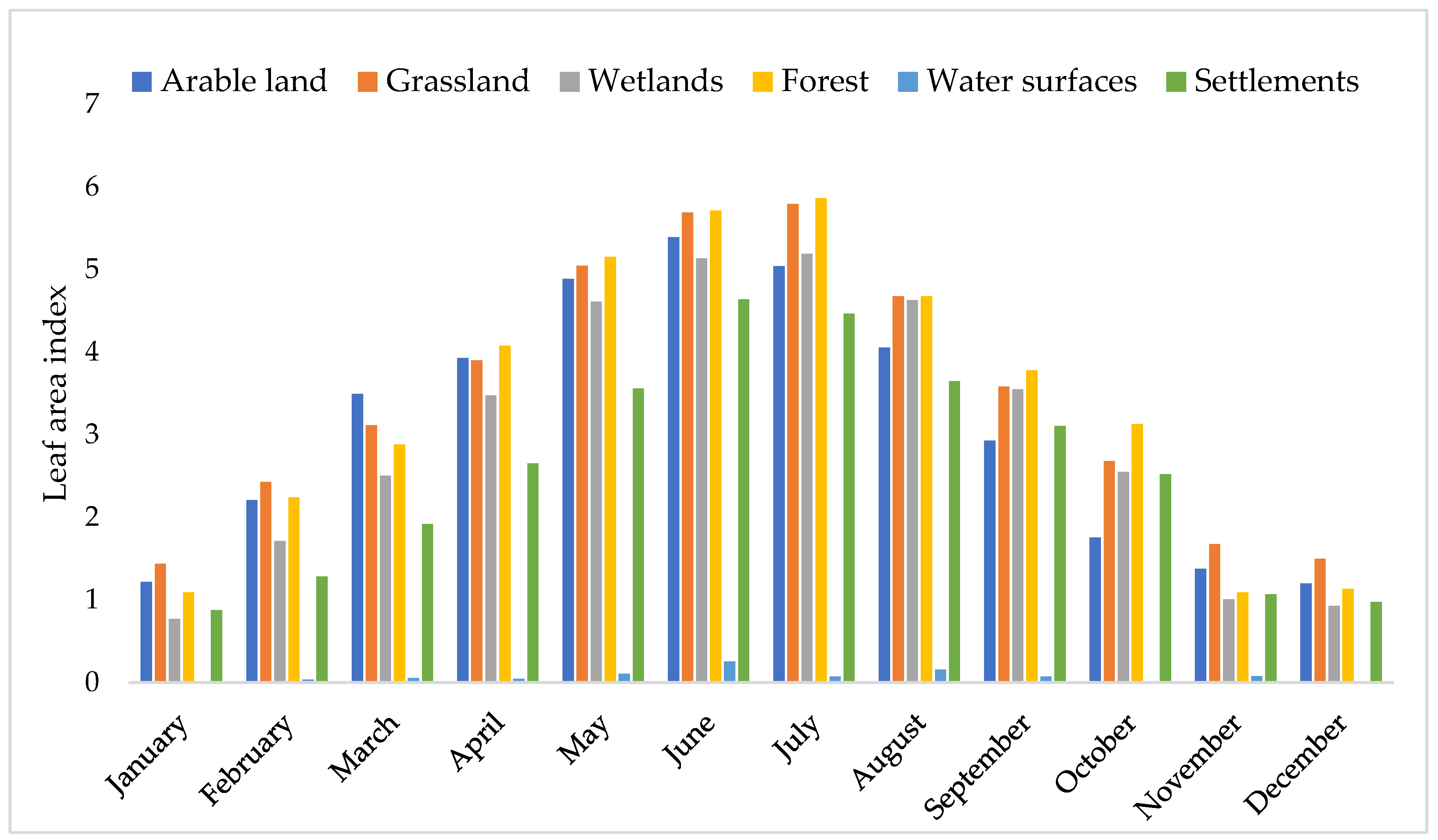
2.2.2. Land-Use Data

Land use is based on Rapid Eye Archive images (https://resa.blackbridge.com). Land-use classification was performed to classify the land use into arable land, forest, grassland, wetland, lakes, and settlement areas. Average root depths (RD) for different land-use classifications during the winter and summer season are shown in

Table 2. Average root depths (RD) for different land-use classes during winter and summer seasons in Augraben River catchment [34].

Land-Use	Average Root Depth in Winter (mm)	Average Root Depth in Summer (mm)
Arable land	200	600
Wetlands	300	300
Grassland	100	300
Forest	800	800
Settlements	600	600
Water surfaces	0	0

. Leaf area index (LAI) in monthly resolution is presented in Figure 3. RD and LAI were collected from the project KOGGE (www.kogge.auf.uni-rostock.de) conducted in a nearby catchment by University of Rostock.

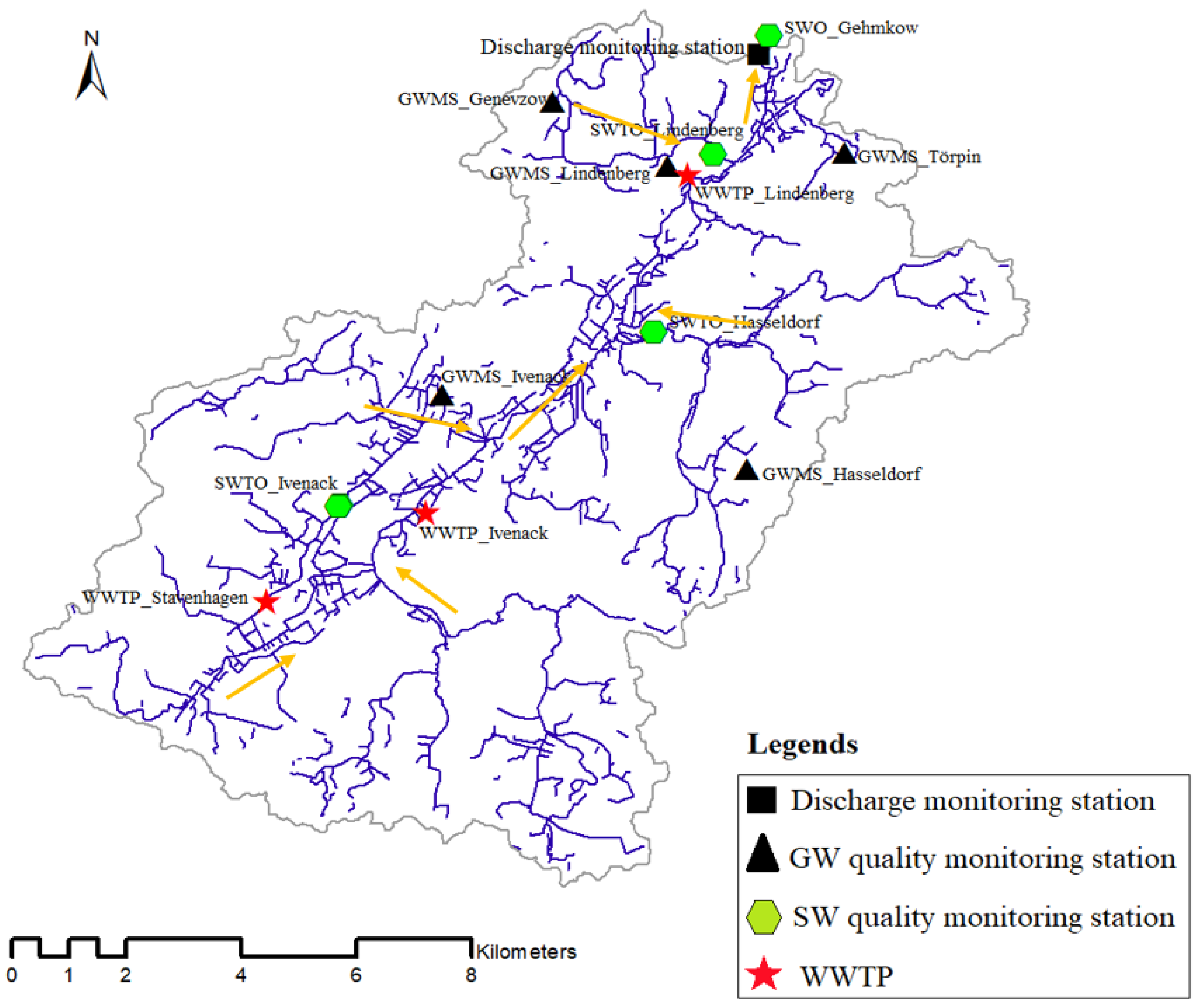
2.2.3. Surface Water Discharge Data

SW flow data at discharge monitoring station Gehmkow were collected from the local environmental protection department (StÄLU-MS) in average daily resolution for a period ranging from 2010 to 2018. Surface flow monitoring station Gehmkow is regarded as Augraben River catchment’s outlet and it summarizes all of the upstream monitoring. No surface flow data were available at other independent tributaries (Lindenberg, Hasseldorf, and Ivenack) contributing to the Augraben River. Figure 4 describes the location of the discharge monitoring station and the main tributaries and their outlets in the Augraben River catchment. The collected observed flow data were used later for flow calibration in hydrological modelling.

2.2.4. Water Quality and WWTP Effluent Data

The locations of available GW and SW quality monitoring stations in the Augraben River catchment are shown in Figure 4.

GW quality data were only available for the GW monitoring stations (GWMSs) named GWMS_Törpin and GWMS_Genevzow, and were obtained from StÄLU-MS in yearly resolution. For this study, additional GW samples were collected at three selected GW monitoring stations (GWMS) named GWMS_Lindenberg, GWMS_Hasseldorf, and GWMS_Ivenack at monthly resolution from January 2017 to December 2017. These water samples were analysed for NO₃-N, NO₂-N, and NH₄-N concentrations. To monitor the GW level, five boreholes were installed at GWMS_Genevzow, GWMS_Lindenberg, GWMS_Ivenack, GWMS_Törpin, and GWMS_Hasseldorf. The GW data loggers provided data with hourly resolution starting from November 2016 to April 2018. Monitored GW levels were used for calibration and validation of the coupled hydrological and hydrodynamic model.

SW monitoring was performed by StÄLU-MS for NO₃-N, NO₂-N, NH₄-N, and P concentrations at the green marked outflows of sub-catchments. The data are available at monthly resolution, but without the according flow data.

Effluent flow volume and NO₃-N and total P concentrations from three WWTPs (WWTP_Ivenack, WWTP, Stavenhagen, and WWTP_Lindenberg) located in the study area were obtained also from StÄLU-MS. SW quality classification was performed by using the German surface water ordinance [35]. The surface water ordinance specifies water quality classes from I (unpolluted) to IV (excessively contaminated).

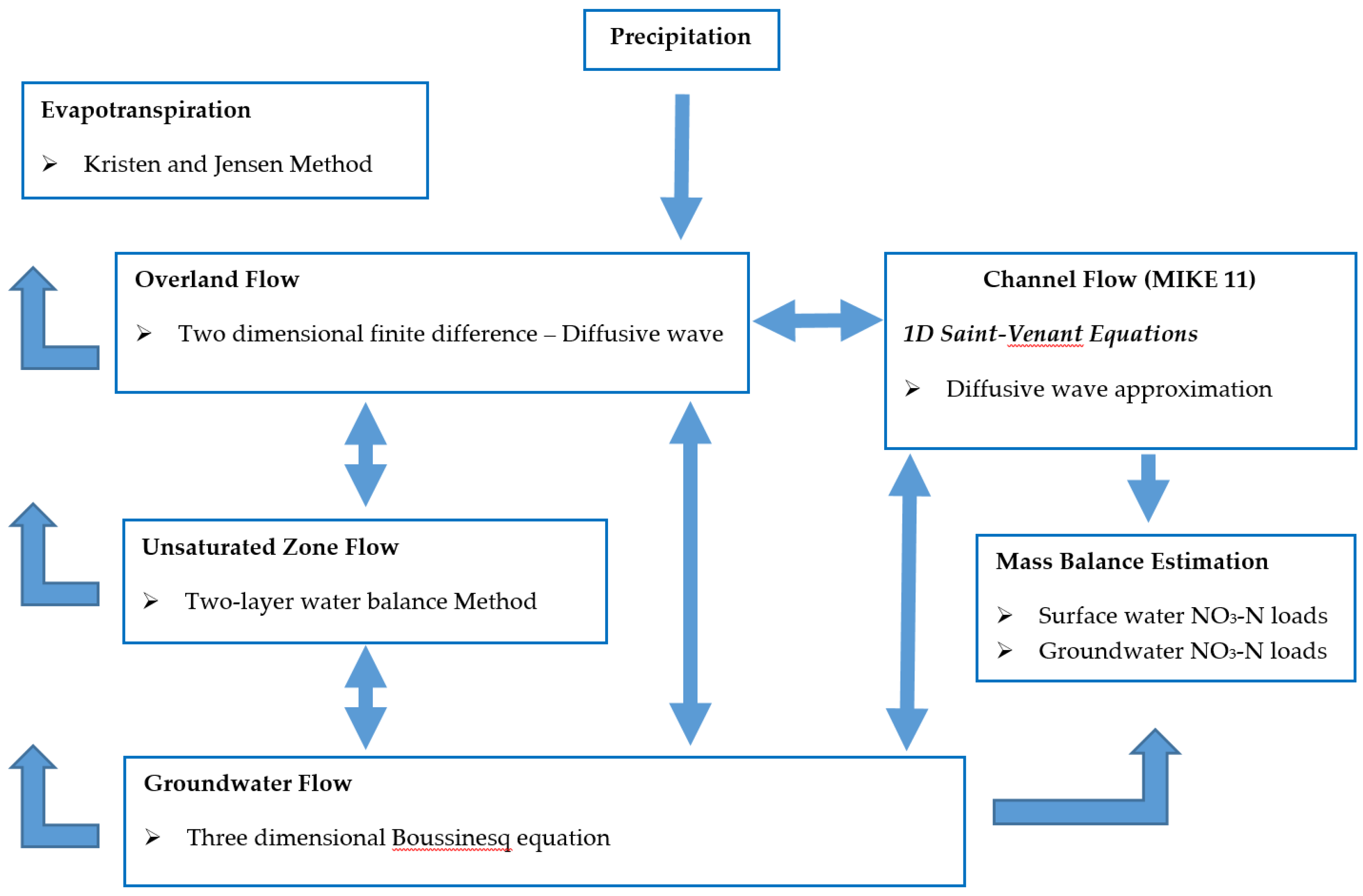
2.3. MIKE SHE Process-Based Modelling and Mass Balance Framework

As discussed above, MIKE SHE was chosen because of its ability to model GW and SW interactions and dynamics within a catchment in a physical and reliable way [36,37]. The modelling framework describing hydrological processes at the desired level of complexity and spatio-temporal variability used in this study is explained in Figure 5. The digital elevation model (DEM) is used as a data development function to define the catchment boundary and stream network. Spatial disaggregation in MIKE SHE is represented by square grids, and the catchment is distributed into grids of equal size. Each square grid is considered homogeneous. Grid-based formulation of MIKE SHE is compatible with grid-based satellite and weather radar data. The soil column is sectioned into three layers: (i) Surface layer, (ii) soil layer, and (iii) groundwater layer in the MIKE SHE model to simulate GW and SW interactions and flows. The MIKE SHE process-based modelling framework includes spatial lumping approaches on catchment and sub-catchment levels. Finally, a hydrodynamic model 11 is coupled with the integrated hydrological model MIKE SHE. MIKE 11 can simulate hydraulic structures. The model framework was also chosen to facilitate the later incorporation of transformation processes using Ecolab. Based on the resulting detailed water balance and simulated SW discharges, SW and GW dynamics and SW and GW NO₃-N loads are estimated [38,39,40].

The hydrological cycle in MIKE SHE is described by a water movement module (WMM). The WMM of MIKE SHE includes precipitation/interception, evapotranspiration (ET), overland (OL) flow, unsaturated zones (UZ), saturated zones (SZ), and exchange between GW and SW. The ET in MIKE SHE is estimated by using the Kristensen–Jensen method. The flow in UZs is modelled by using a two-layer water balance method. SZ flows in MIKE SHE are simulated by using 3D Boussinesq equation. Simplified diffusive wave approximation of the Saint-Venant equation is used to simulate the river hydrodynamics. The coordinate system “ETRS_1989_UTM_Zone_33N_8stellen”, in metric units, is used in this study. Based on the computational time and resulting model performance, the catchment area is divided into 50 × 50 m grids. The topography in the study area is represented by a digital elevation model (DEM) at 5 m resolution and was provided by StÄLU-MS. Zero-flux and GW inflow and outflow gradients are used as aquifer boundary conditions (BC), as shown in Figure 6a. Catchment boundaries where lateral flows were likely to be negligible based on GW contours are defined as zero-flux BC. However, catchment boundaries where GW lateral inflow and outflow were expected are defined as positive and negative GW gradient BC. The geology is based on borehole log data and is mainly represented by three geological layers in the SZ of Augraben River catchment. The borehole log data from the available 23 boreholes in the study area were used to define the aquifer depth. The river network containing the Augraben River and its tributaries is defined in MIKE 11, as shown in Figure 6b. The coupling of MIKE SHE and MIKE 11 was done dynamically by considering the exchange of data between river links in MIKE 11 to the adjacent MIKE SHE grids after every computational time step [41].

3. Results

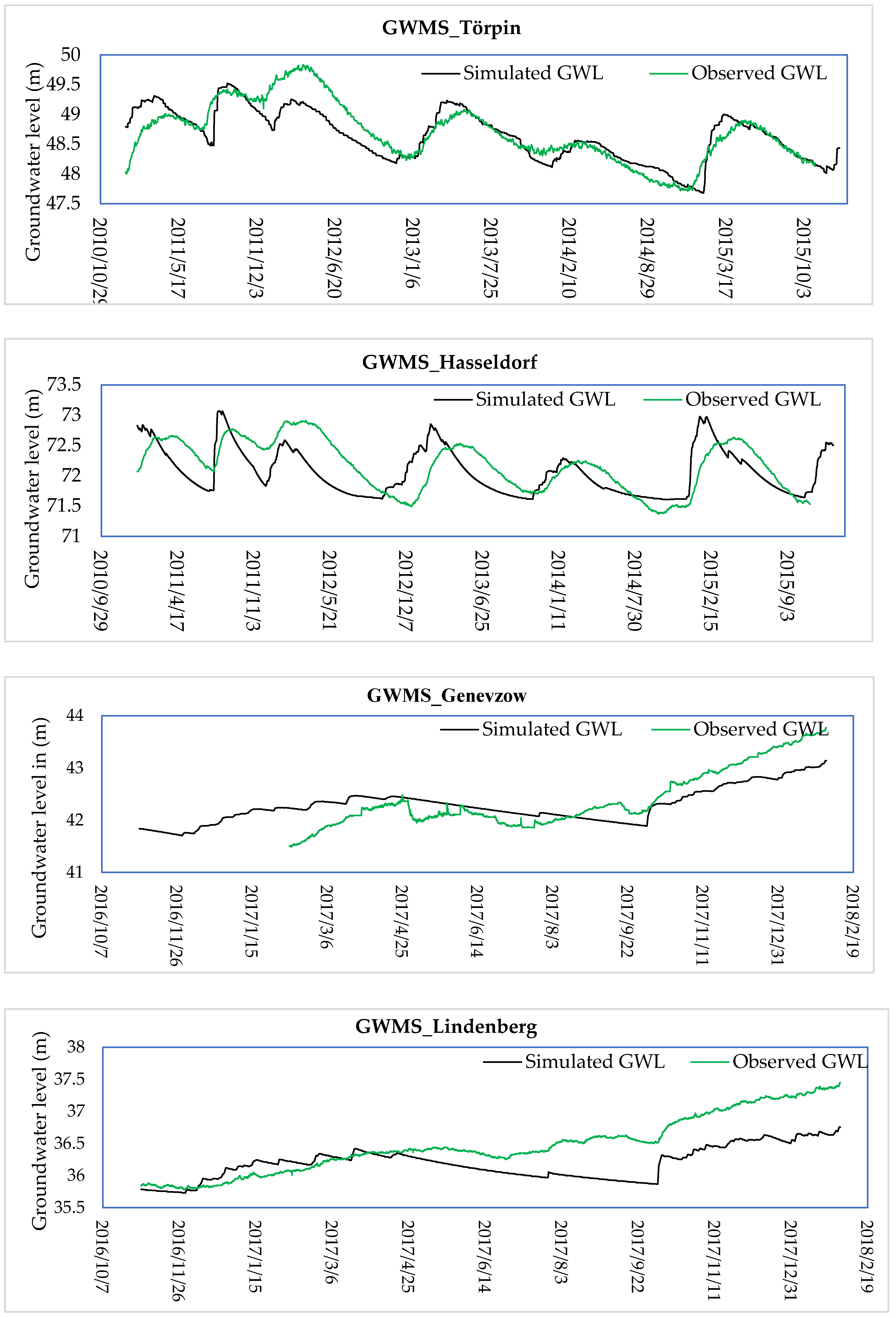
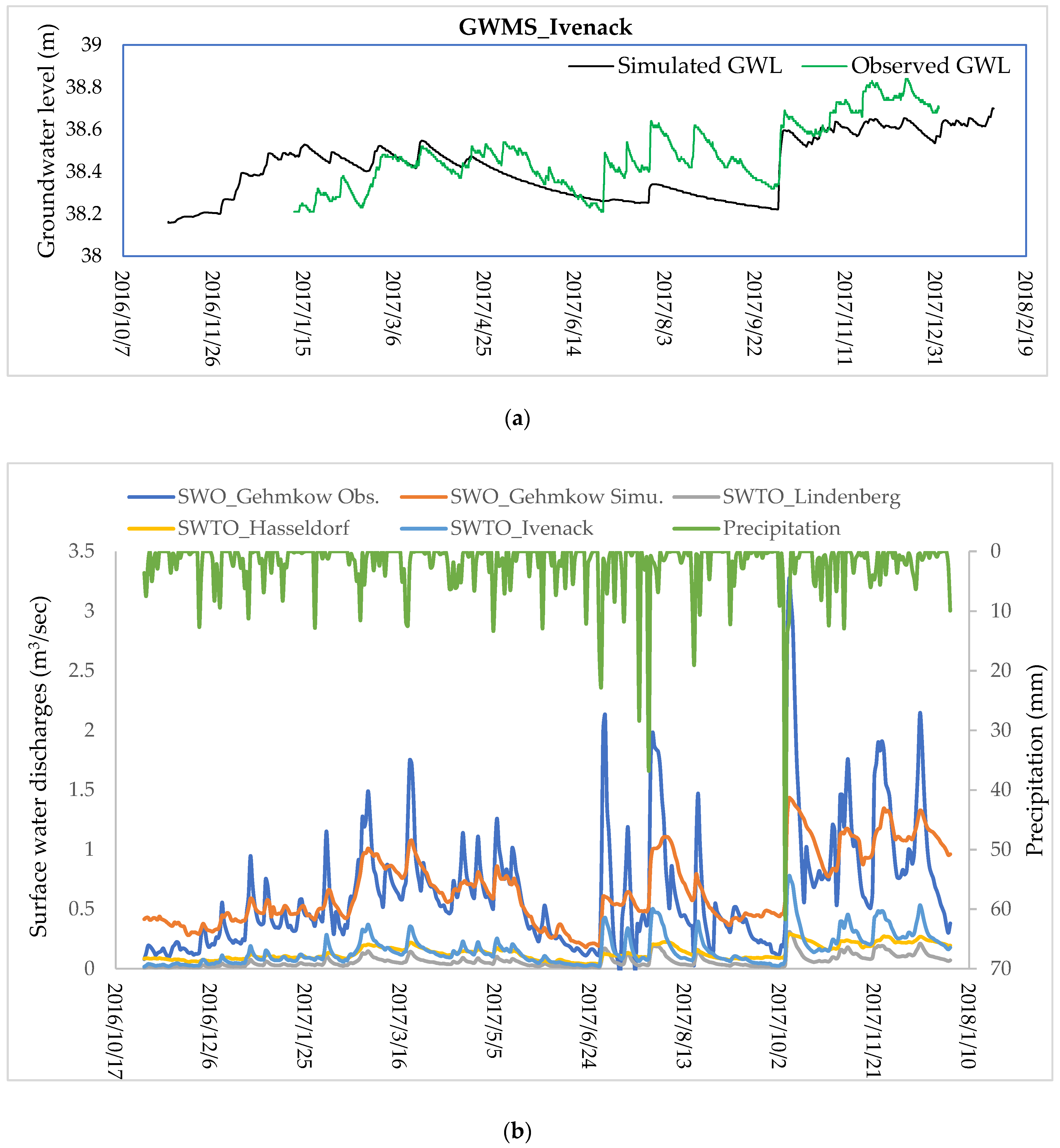
3.1. Coupled Hydrological and Hydraulic Model Calibration and Validation

The most sensitive parameters for the Augraben River catchment were assessed by sensitivity analysis. Sensitivity analyses were performed by adjusting one parameter value at a time, while keeping others constant in a particular simulation; the magnitude of impact on the simulated results was evaluated for every single parameter value adjustment/change. The resulting most sensitive parameters include initial potential heads, BCs, and saturated hydraulic conductivity. Hourly monitored GW levels (January 2011–December 2015) at GWMS_Törpin, GWMS_Hasseldorf, GWMS_Genevzow, GWMS_Lindenberg, and GWMS_Ivenack were used for the calibration of simulated GW levels by using monitored GW levels (November 2016–April 2018). After calibration, the coupled MIKE SHE and MIKE 11 model was used for generating discharges at ungauged locations.

Table 3. Calibration parameters, their ranges, final values, and statistical performance of the coupled model.

Calibration Process
Selected Parameters	Initial Input Value		Input Range	Calibrated Value
Hydraulic conductivity [m/s]	A: 1 × 10−6 B: 1 × 10−8 C: 1 × 10−10		1 × 10−10–1 × 1010 1 × 10−10–1 × 1010 1 × 10−10–1 × 1010	1 × 10−4 1 × 10−7 1 × 10−10
Specific yield	A: 0.25 B: 0.2 C: 0.1		1 × 10−10–1 × 1010 1 × 10−10–1 × 1010 1 × 10−10–1 × 1010	0.266 0.20 0.108
Boundary condition Groundwater inflow and outflow gradients	+ve gradients: 0.0015 −ve gradients: 0.004		0.009–−0.009 0.009–−0.009	0.0036 −0.004
Manning roughness coefficient	Natural channel: 10 Weirs or concrete surfaces: 80		10–25 80–100	15 85
Statistical performance of groundwater calibration
Monitoring Station	MAE (m)	RMSE (m)	R (Correlation)	STDres
GWMS_Genevzow	1.467	1.508	0.845	0.352
GWMS_Ivenack	1.159	1.166	0.749	0.131
GWMS_Lindenberg	0.478	0.557	0.786	0.351
GWMS_Hasseldorf	1.09	1.107	0.7403	0.24
GWMS_Törpin	1.500	1.555	0.646	0.411
Statistical performance of river flow calibration
Monitoring Station	MAE (m3/s)	RMSE (m3/s)	R (Correlation)	STDres
SWO_Gehmkow	0.4514	0.5799	0.7797	0.5299

MAE = “mean absolute error in meters”; RMSE = “root mean square error in meters”; R = “correlation”; STD = “standard deviation residuals”.

describes the calibration parameters, initial and calibration value ranges, selected calibrated values, and statistical performance of GW and SW calibration and validation. Simulated and observed GW levels and SW discharges are shown in Figure 7a,b, respectively. Coupled hydrological and hydraulic model performance was evaluated by using mean absolute error (MAE), root mean square error (RMSE), correlation coefficient (R), and standard deviation residuals (STDres).

The simulated results show that GW levels are high during the winter and low during the summer season due to respective low and high ET rates. In the current study, the coupled MIKE SHE and MIKE 11 model underestimated the GW levels during high recharge periods. However, model performance was not equally comparable at all monitoring locations, but showed a strong spatio-temporal relationship between simulated GW levels and observed climatic data (precipitation, ET). First, we compare the flow with the only available monitoring station in Gehmkow. Here, the volume balance is met well, while the dynamics are underestimated during high flows and overestimated during low flows with an R² (Nash Sutcliff) of –0.873687. This possibly happens due to the provision of artificially constructed drainage in MIKE SHE based on the lowest DEM points. The constructed drainage does not fully reflect the installed drainage in the Augraben River catchment; Figure 1 shows the branched drainage system used in this study. Drainage becomes ineffective when the GW levels fall below the provided artificial drainage levels in MIKE SHE, resulting in smaller GW contribution to the Augraben River and its tributaries. Afterwards, the calibrated model was applied to calculate flows at the ungauged locations.

3.2. Water Balance Estimation

A detailed yearly water balance was performed for the Augraben River catchment for 2010–2018. Each hydrological year was considered from 1 October to 30 September of the upcoming year based on local conditions. In this study, the hydrological model gets its total water input via precipitation and SZ GW inflow. The total water budget was further divided into ET, surface runoff, change in UZ and SZ storage, and GW and SW interactions. Water balance error was estimated based on total inflows (precipitation, surface and subsurface GW inflow), outflows (ET, overland flow, surface and subsurface GW outflow, GW and SW interactions), and change in UZ and SZ storage. The water balance error of 2% during the calibration period shows the suitable model performance during the simulation period of 2010–2018. Detailed water balance results show that ET loss represents an approximate average of 60–65% of the total precipitation in the study area. The GW contribution to the Augraben River and its tributaries as a base flow and the SW contribution to the GW as infiltration and percolation show the exchange of flows between MIKE SHE and MIKE 11. SW discharge is mainly fed by GW. The GW contribution to total SW discharges accounts for up to 85–95%. The water balance results show a small decrease in SZ storage over the period of the last eight hydrological years.

Table 4. Water balance for the Augraben catchment (90 km²) during hydrological years 2010–2018; all values are in millimetres (mm).

Water Balance Components (mm)	2010–2011	2011–2012	2012–2013	2013–2014	2014–2015	2015–2016	2016–2017	2017–2018	2010–2018
Precipitation	804	511	597	573	599	502	767	447	4814
Evapotranspiration	473	376	445	456	401	367	482	316	3324
Canopy storage change	0	0	0	0	0	0	0	0	0
Overland flow to the river	59	38	37	26	35	34	37	44	311
Snow storage change	0	0	0	0	0	0	0	0	0
Overland storage change	8	−2	−4	2	1	0	6	−7	5
UZ storage change	−24	20	−6	6	1	−26	29	−44	−42
SZ storage change	22	−146	−80	−95	−21	−50	39	−53	−388
SZ drain to river	123	90	79	62	68	66	68	79	638
Infiltration	373	138	182	124	213	180	264	204	1681
Exfiltration	88	61	58	42	54	53	52	68	477
UZ boundary inflow	0	0	0	0	0	0	0	0	0
UZ boundary outflow	3	1	1	1	1	1	2	2	13
SZ boundary inflow	61	55	50	43	43	42	38	43	377
SZ boundary outflow	202	187	175	159	155	152	143	152	1330

shows the detailed water balance for the Augraben River catchment; all values are in millimetres (mm). Positive and negative storage change represents the ascending and descending change in water stored in SZ and UZ.

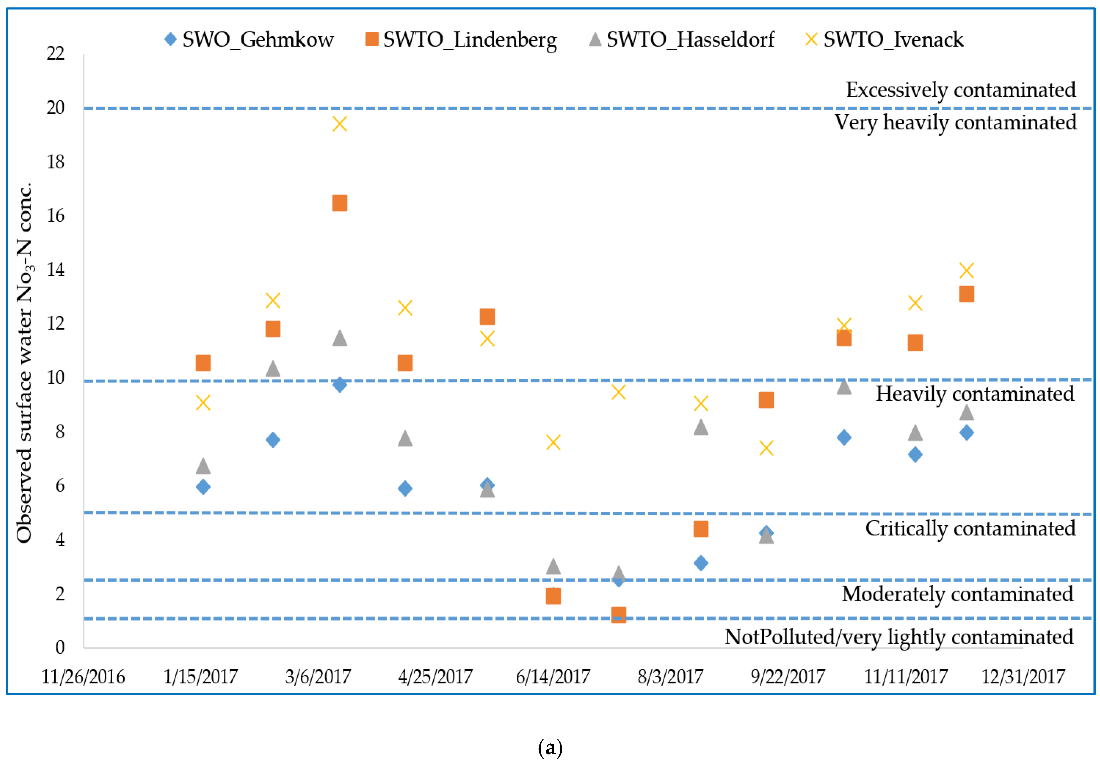
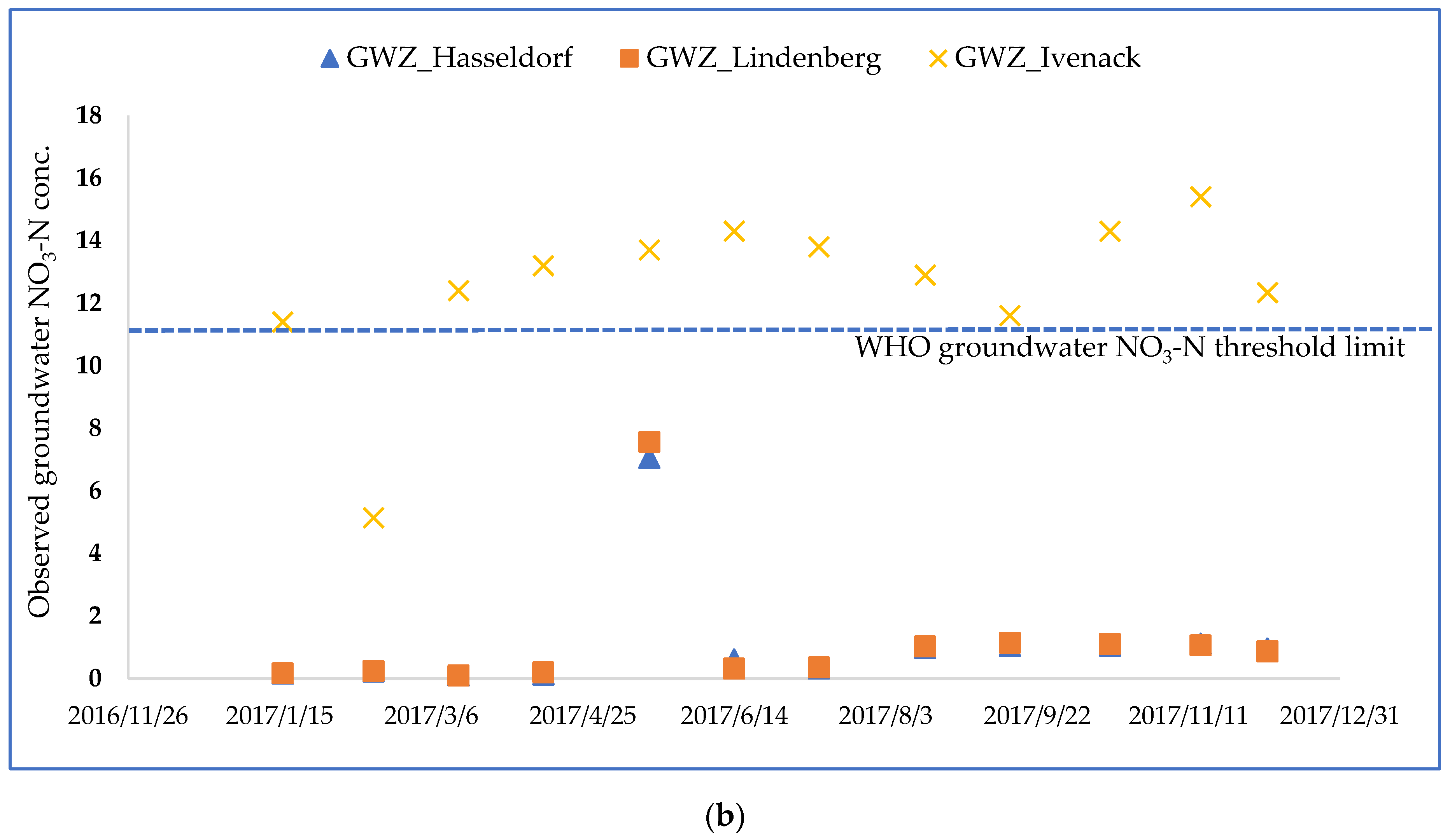
3.3. Surface Water and Ground Water Quality

Observed SW and GW quality data in Augraben River catchment were partially measured (at officially existing monitoring locations) and partially obtained from the local environmental protection department in Augraben River catchment. Observed SW and GW NO₃-N concentrations were distributed into pollution classes according to the federal surface water ordinance [35] and the World Health Organization’s (WHO) [15] guidelines for NO₃-N in GW, respectively. In terms of SW quality, 35.41% of the collected SW samples showed NO₃-N concentrations belonging to the category of very heavily contaminated rivers. A total of 43.75% of the SW samples fell under the category of heavily contaminated and 6.25% moderately contaminated. None of the SW samples showed concentrations belonging to the category of lightly or non-polluted rivers. Observed NO₃-N concentrations and their respective pollution categories are shown in Figure 8. Classification at the tributary scale shows that measured NO₃-N concentrations at the tributary outlets named SWTO_Lindenberg and SWTO_Ivenack come under the water quality class of very heavily polluted, as the measured NO₃-N concentrations are clearly elevated, and concentration is reduced only in months from June to September, but still lies in the category of heavily polluted rivers. For approximately similar land-use conditions in the study area, low SW NO₃-N concentrations were observed at SWTO_Hasseldorf. This shows that the SWTO_Lindenberg and SWTO_Ivenack water quality monitoring stations were possibly influenced by the point sources contributing to SW pollution. The observed SW NH₄-N concentrations also lie in the category of very highly contaminated rivers. In terms of GW NO₃-N concentrations, 30% of the GW samples collected in the study area in 2017 showed higher concentrations then the threshold limit defined by the WHO for GW. GW quality classification shows that the GW zone (GWZ) Ivenack NO₃-N concentrations throughout the year are higher than the threshold value of 11.3 mg/L defined by the WHO. However, GWZ_Lindenberg and GWZ_Hasseldorf show lower NO₃-N concentrations.

ET follows the intensity of incoming solar radiation and the resulting number of sunshine hours during the course of the year. Low ET in combination with moderate precipitation during the winter and spring seasons results in higher discharges. Fertilizer is applied primarily in spring and (to a lower extent) in early autumn, and plant nitrogen uptake follows the pattern of ET in the study area. Total monthly NO₃-N loads at SWO_Gehmkow follow the seasonal pattern of the total monthly runoff volume. GW quality monitoring is influenced by various factors. Observed NO₃-N concentrations at a particular GWMS do not wholly represent the water quality status of a GWZ. The reliability of GW monitoring is influenced by the selection and location of the boreholes [42,43]. In the study area, qualitative monitoring was performed at two hydrological boreholes bi-yearly and at three boreholes monthly. MIKE SHE coupled with a hydrodynamic model MIKE 11 simulated the GW levels and flow directions in the study area. In order to quantify the representative area of the saturated zone under each monitored borehole, the calibrated GW model MIKE SHE coupled with a hydrodynamic model MIKE 11 was applied to estimate GW flow directions. The constructed GW contours explain that the GW flow direction is towards the Augraben River and its tributaries throughout the catchment, and that underlines that GW largely contributes to the surface discharges. However, GWZ_Ivenack is special, as GW contributes to the tributary and also passes underneath the river towards lower GW elevations. The GW table, in general, follows the topography of the catchment; however, in some areas, it differs from the topography. Water in the saturated zone flows due to differences in the energy state of the water, described by the term hydraulic head. The GW flow is determined by the gradient in the hydraulic head and the hydraulic conductivity, which is an empirical constant describing the ability of geological media to transmit water. Based on GW flow directions and available GW monitoring stations in the study area, the representative area was estimated according to each available GW quality monitoring station. The Augraben River catchment is divided into three GWZs (GWZ_Lindenberg, GWZ_Hasseldorf, and GWZ_Ivenack), as shown in Figure 9. The boreholes named GWMS_Genevzow and GWMS_Lindenberg are located in GWZ_Lindenberg, boreholes GWMS_Törpin and GWMS_Hasseldorf are located in GWZ_Hasseldorf, and GWMS_Ivenack is located in the GWZ_Ivenack. GW flow paths vary greatly in length and depth depending on where the GW recharges and the travel time within a catchment. In highly polluted areas, it is necessary to conduct reliable monitoring of GW, as better GW quality assessment will help in counteracting the negative effects of pollution [44,45,46,47].

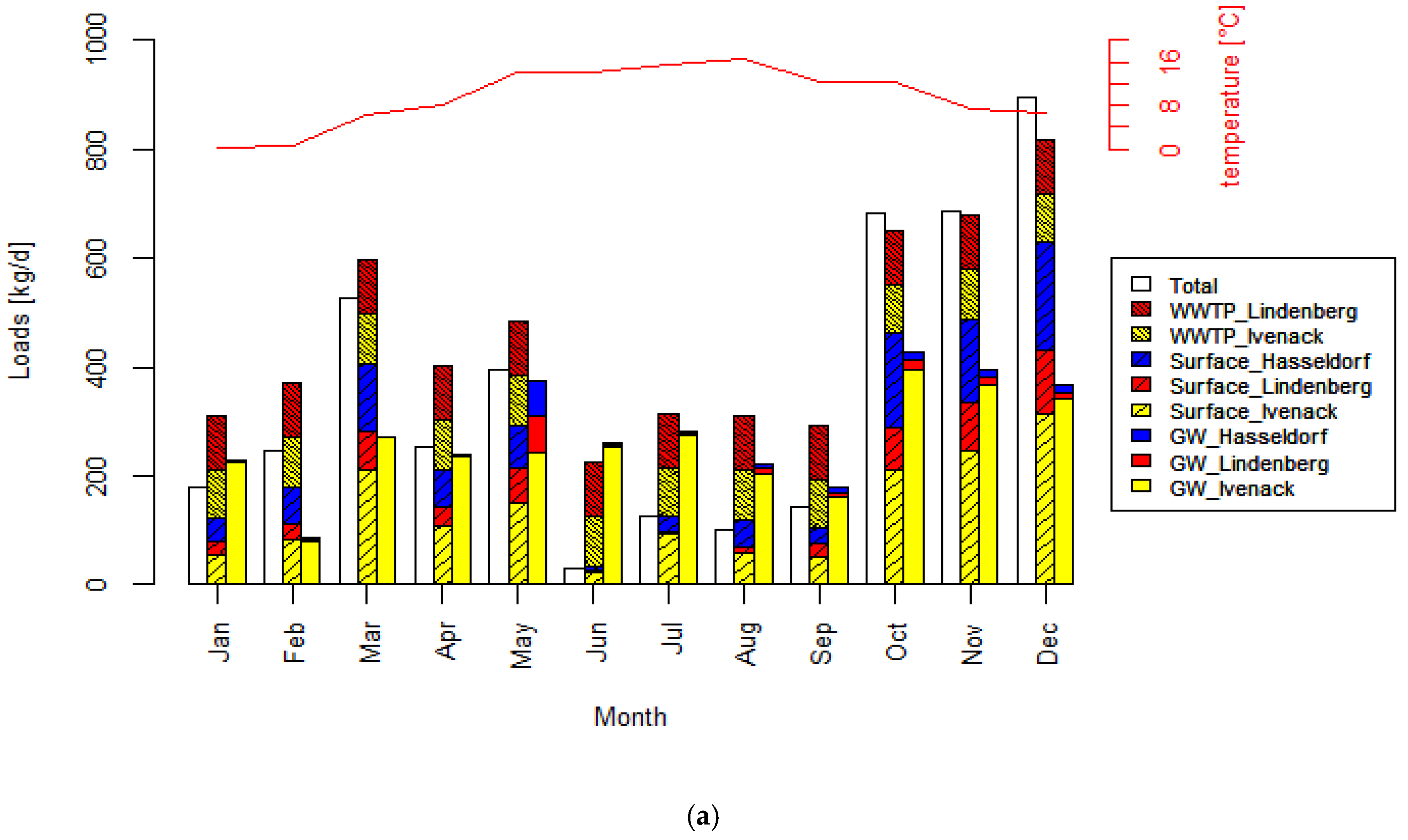
3.4. Nutrient Balance at Catchment Outlet

The uncertainties in average concentration and load estimations can be reduced by increasing the sampling frequency. However, the SW and GW sampling, sample transport, and laboratory procedures are expensive and laborious. A favourable approach is the load estimation from available observed low-frequency concentration data. The explanatory strength of commonly available continuous measurements, such as precipitation, discharge, and GW levels at limited locations, in combination with hydrological modelling can access water quality variation at ungauged locations. Most of the commonly available hydrological measurements (precipitation, temperature, wind speed, etc.) are relatively inexpensive and often available near SW and GW quality monitoring locations to facilitate the quantitative management of water. First, simulated SW discharges obtained from the coupled MIKE SHE and MIKE 11 model were used to estimate the SW NO₃-N, NO₂-N, NH₄-N, and total P loads at SWTO_Lindenberg, SWTO_Hasseldorf, SWTO_Ivenack, and SWO_Gehmkow. WWTPs and their effluent NO₃- N and total P loads were added to estimate the NO₃-N balance and NO₃-N transformations at the Augraben River outlet. Secondly, simulated GW flows for each respective GWZ were used to calculate the GW NO₃-N loads in all three GWZs, named as GWZ_Lindenberg (red), GWZ_Hasseldorf (blue), and GWZ_Ivenack (yellow). It is estimated that GWZ_Lindenberg and GWZ_Hasseldorf contribute the least to the GW NO³-N loads, while GWZ_Ivenack, based on measured concentrations and GW volumes, contributes a maximum of up to 96% in terms of GW NO₃-N loads. The possible causes behind the higher observed GW NO₃-N concentrations at GWZ_Ivenack in comparison to GW NO₃-N concentrations at GWZ_Lindenberg and GWZ_Hasseldorf include (1) infiltration from two nearby WWTPs, where WWTP_ stavenhagen is a large-scale WWTP, and effluent NO₃-N load discharged into the tributary Ivenack can infiltrate into the GW. As NO₃-N loads are detectable at SWTO_Ivenack, that is why WWTP NO3-N loads are not specified separately in Figure 10a. Total effluent NO₃-N loads from WWTP_Stavenhagen account for 47.84 kg/d. Direct GW infiltration is negligible or zero, as WWTP_Stavenhagen does not allow GW infiltration due to its construction and operational design. WWTP_Ivenack is a pond-type WWTP and can possibly influence the GW quality due to infiltration. However, its small-scale operational capacity also limits its possible contribution to GW quality. Stormwater runoff from biogas plants and other agricultural facilities was identified in other studies as a potentially relevant pollution source [48]. As the land use type is nearly the same in the Augraben River catchment, higher GW concentration could also point to a different fertilizer usage behaviour in different areas of the catchment. A high spatio-temporal monitoring is necessary to evaluate the GW and SW quality variation at a smaller scale, but it is evident from the estimated GW loads that the highest GW loads occur in June, July, August, and September.

The nutrient balance of the estimated SW loads at the Augraben River outlet is shown in Figure 10a. It reveals that, especially in summer, the total NO₃-N loads at SWO_Gehmkow are lower than the sum of the calculated SWTO_Lindenberg, SWTO_Hasseldorf, SWTO_Ivenack, and WWTP effluent loads. Here, an inverse relationship between NO₃- N loads and observed water temperature is visible. The higher reduction in SW NO₃- N loads at the outlet during the summer months indicates significant transformation either by denitrification or by increased plant growth. In winter or during times with low water temperatures, the biological processes are reduced to a very low level while base flow increases, resulting in higher nitrate loads. The difference between total SW loads at SWO_Gehmkow and the summed loads from SWTO_Lindenberg, SWTO_Hasseldorf, SWTO_Ivenack, and WWTP gives the magnitude of the transformation and plant uptake, on average, of up to 50% of total loads at SWO_Gehmkow during the months of June, July, August, and September. The loads of NO₂-N, NH₄-N, and total P are shown in Figure 10b. In general, SWO_Gehmkow’s water quality status lies in the strongly polluted river category.

The main findings of nutrient balance at SWO_Gehmkow include (1) estimation of SW and GW loads from each SWTO and representative GWZ; (2) estimation of NO₃-N transformation and plant uptake rate; (3) critical SW and GWZ identifications requiring maximum measures to reduce NO₃- N loads; (4) explanation of possible NO₃-N hotspots influencing the water quality. It is recommended that the locations of water quality monitoring stations should be reconsidered based on tributaries with heavy pollution and GW flow directions to accurately point out the hotspots. This study highlights the need for further necessary measures to achieve the EU-WFD goals and demands a stronger process-oriented monitoring. A valuable improvement would already be flow measurement in parallel with grab sampling.

4. Discussion

The bi-directional coupled hydrologic (MIKE SHE) and hydraulic (MIKE 11) model was applied to the Augraben River catchment, a tributary of the Tollense River. The Augraben River catchment represents common features of the European lowland catchments, such as shallow GW tables, GW and SW interactions, control structures, provision of artificial drainage, periodic inundation, etc. Due to these features, the modelling approach explained in the current study has a huge potential to simulate/predict the lowland response to anthropogenic activities and expected changing climatic conditions and to provide guidelines for better conservation and management practices of susceptible catchments.

4.1. Method Strengths

Water Balance: Water balance estimation in a river catchment predicts the detailed surface water and groundwater interactions. A detailed water balance explains the main water loss components and will help in developing watershed management practices and better informed policy decisions [49,50]. In this study, the calibrated coupled MIKE SHE and MIKE 11 model has predicted the water balance with an error of less than 2%. ET is a main water loss component. Surface discharges are mainly fed by groundwater, and groundwater flow is a dominant pathway in the Augraben River catchment. Higher groundwater contributions to surface water discharges in lowland Augraben River catchment are following the hydrological studies conducted in lowland catchments in north-eastern Germany [1,51,52,53]. Overland flow or direct runoff is very low in comparison to other water balance components. Lowland catchments are characterized with low direct runoff flows in contrast to mountainous catchments, where direct surface water runoff is a dominant pathway [54,55]. The resulting groundwater contribution to surface groundwater and surface water interactions mainly controls the pollutant (NO₃-N) dynamics and influences the surface water and groundwater quality [56,57].

Simulated Surface Flow at Ungauged Locations and Groundwater Levels: The lack of surface water discharge monitoring stations in small or remote catchments is a hurdle in defining the catchment management measures [58,59]. In the Augraben River catchment located in north-eastern Germany, discharge data were only available at the catchment outlet. No measured discharges were available at the Augraben River’s tributaries. In the current study, the groundwater levels and surface discharges were successfully generated by the integrated coupled hydrological and hydraulic model (MIKE SHE and MIKE 11). The simulated discharge at Gehmkow shows good agreement between simulated and observed discharge with an R (correlation) of 0.7797 and RMSE of 0.579. The performance of the calibrated model is not the same at all locations due to the defined simplifications during the modelling procedure.

Mass Balance and NO₃-N Transformation Rates: The NO₃-N pollution of SW and GW is a major environmental problem, especially in lowlands with intensive agriculture and related farm activities. Achievement of environmental sustainability requires the detailed assessment of spatial and temporal variation of water quality at the catchment and regional scale. River mass balance methods using observed or simulated flows and pollutant concentrations can be helpful in describing the magnitude and extent of existing pollutant loads along a river [60,61]. Based on coupled hydrological and hydraulic model results, we have successfully estimated the NO₃-N loads at the catchment and sub-catchment scale by combining low-frequency monitoring data with hydrological modelling. GW levels were available at only two monitoring stations. In terms of water quality assessment and its variations at a catchment scale, limited monitoring data were available. This enhances both the explanatory strength of generally available and inexpensive quantitative hydrological data and the (so far, only) qualitative status information from grab sampling [62]. The responses of NO₃-N and P concentrations can be plausibly linked to the hydrological dynamics of SW and GW, triggered by the meteorological input. Combining these data with measured emission data of WWTP, a trustworthy source apportionment between diffuse and known point sources is feasible. In summertime, the measured load is lower than the predicted sum. The difference can be a rough estimate of NO₃-N transformations and plant uptake rates. The results of this study demonstrate, in line with similar studies [63,64], that using the explanatory strength of quantitative hydrological data can significantly improve load estimates.

4.2. Method Weakness

Short-term dynamics of SW quality variations are not captured by common low-frequency grab sampling. The low-frequency monitoring provides an overview of the average concentrations of chemical species and suggests some general processes that may explain the observed data. The added value of high-frequency monitoring is the possibility of capturing diurnal cycles and transient events that help relate the causes and effects of human activities and storms. High-frequency monitoring can go much further in the interpretation of the data and can more precisely uncover and/or confirm rapid processes at work in the system [65,66,67]. The method can reliably estimate the contribution of diffuse sources. To explain loads from point sources, additional data are needed. Here, only the data of WWTP emissions could be included. Polluted storm water runoff could be an additional nutrient input, which was not addressed so far.

From the qualitative perspective, the method is purely data-driven. It could be considered to expand the hydrological model by additional transformation processes. This was out of the scope of this study, aiming at an improved interpretation of available monitoring data. However, with regard to designing mitigation measures, an expanded process model would be worthwhile.

4.3. Transfer of Methodology to Other Lowland Catchments

The method of the applied coupled hydrological model in combination with low-frequency monitored data can be transferred at the desired rate of complexity to similar lowland catchments. According to our assessment, the chosen model setup was best suited to simulate the typical characteristics of lowland catchments, such as (i) artificial drainage to support better agriculture activities, (ii) backwater effect due to smaller slopes, (iii) complex SW and GW interactions, and (iv) river flows. The subsequent mass balance and source apportionment are valuable to prioritize and allocate measures to reduce nutrient emissions.

However, the method is not delimited to the model framework chosen here. Under different boundary conditions, other models could be equally or even more advisable. Four different process-based models—“soil and water assessment tool” (SWAT), “soil and water integrated model” (SWIM), “hydrological simulation program—FORTRAN” (HSPF), and a coupled “MIKE SHE and MIKE 11” model—were compared in this study. The DHI’s combined tools and SWAT were more suitable for simulating the desired hydrological processes, but in the case of river hydraulics, the integrated coupling between MIKE SHE and MIKE 11 is a plus. In the case of SWAT, it needs to be coupled with another tool to model the hydraulics in the Augraben River, as SWAT does not simulate the backwater effects and operation of control structures (weirs, gates, etc.). However, both the SWAT and DHI tools are more data-demanding in comparison to SWIM and HSPF. HSPF, in turn, already contains tools to model nitrogen transformation and transport processes along the hydrological system, which is helpful for designing mitigation measures. Most of the input data and governing equations in the case of SWIM and SWAT are similar. SWIM does not simulate water bodies (ponds and lakes), wetlands, and drainage systems.

4.4. Usefulness of Model Predictions and Future Applications

The analysis of the model’s predictions/future forecasts and deficiencies related to model structure and availability of data offers better understanding of the processes (water and nutrient) at different temporal (monthly and annual) and spatial scales (catchment, sub-catchment, river). In the Augraben River catchment, critical areas were identified where in-depth additional investigations are required. In particular, the specific emissions in the Ivenack sub-catchment were noticeably higher than in the other sub-catchments. Accordingly, monitoring and systems analysis should be strengthened here to support better catchment management practices/activities. As expected, higher NO₃-N loads occur outside the vegetation period during autumn and winter. Estimated NO₃-N loads are heavily influenced by temperature. The differences between forecasted and measured nitrate loads in SW can be interpreted/transformed/removed; loads are very low during the winter and autumn seasons due to the lower temperatures. Environmental conditions during the summer and spring seasons favour higher plant uptake and increased microbial activities.

4.5. Key Parameters to Reduce Nitrogen Inputs

The study was performed in the phase when the new fertilizer regulation came into effect. The observed state still represents the conditions before the stronger regulations. It can be assumed that the reduced tolerated nitrogen surplus will, in the longer term, be viable in reduced nitrogen concentrations at the GW, and will accordingly reduce loads to the SW. The increased specific loads from the Ivenack catchment may not only be due to farming activities. For several years, polluted stormwater runoff from sealed areas on animal farms and biogas plants has been suspected to be an important nutrient point source. In addition, the view should be open to so far unidentified polluters. Regular water quality monitoring and sampling frequency at a higher resolution will help in reliable and precise assessment of the status of surface and groundwater bodies.

5. Conclusions

The NO₃-N pollution of SW and GW is a major environmental problem, especially in lowlands with intensive agriculture and related farm activities. Achievement of environmental sustainability requires the detailed assessment of spatial and temporal variation of water quality at the catchment and regional scale. The required high-resolution spatial and temporal monitoring for profound assessment is often in contrast the existing data. This study, conducted in a north-eastern German lowland catchment, aims at improving the expressiveness of inconsistent monitoring data by combining it with a coupled hydrologic model. The main conclusions are:

• By combining a coupled SW/GW model with spatially and temporally scarce grab samples, the dominant nutrient entry pathways can be roughly allocated and quantified.
• Process-based hydrological modelling can help in defining SW and GW quality monitoring locations and schedules.
• The modelling approach can be transferred to similar lowlands, and a calibrated coupled model can be used to identify the priority areas to reduce nutrient pollution. Differences between accumulated loads and measured total loads can be used as rough estimates for instream transformation processes.

The SW quality in the investigated Augraben River system varies—applying national and international assessment schemes—between moderately to very heavily polluted. Total load reached a maximum NO₃-N load of 650 kg/d in 2017. In the summer season, GW loads’ contribution is higher in comparison to the total load at the catchment outlet. However, in winter, a higher SW load is calculated with a small increase in GW load. NO₃-N loads from point sources, such as WWTP, cannot be neglected. In this study, estimated GW loads in GWZ_Ivenack contributed the most to the total GW loads. WWTP_Stavenhagen, on average, contributes 25% of the total NO₃-N load at SWTO_Ivenack. Areas with higher NO₃-N loads (GWZ_Ivenack in this study) require maximum water quality improvement efforts to reduce high NO₃-N levels.

References

1. Lam, Q.D.; Schmalz, B.; Fohrer, N. Assessing the spatial and temporal variations of water quality in lowland areas, Northern Germany. J. Hydrol. 2012, 438, 137–147. [Google Scholar] [CrossRef]
2. Schmalz, B.; Springer, P.; Fohrer, N. Variability of water quality in a riparian wetland with interacting shallow groundwater and surface water. J. Plant. Nutr. Soil Sci. 2009, 172, 757–768. [Google Scholar] [CrossRef]
3. Krause, S.; Bronstert, A.; Zehe, E. Groundwater–surface water interactions in a North German lowland floodplain–implications for the river discharge dynamics and riparian water balance. J. Hydrol. 2007, 347, 404–417. [Google Scholar] [CrossRef]
4. Hesse, C.; Krysanova, V.; Päzolt, J.; Hattermann, F.F. Eco-hydrological modelling in a highly regulated lowland catchment to find measures for improving water quality. Ecol. Model. 2008, 218, 135–148. [Google Scholar] [CrossRef]
5. Sophocleous, M. Interactions between groundwater and surface water: The state of the science. Hydrogeol. J. 2002, 10, 52–67. [Google Scholar] [CrossRef]
6. Kieckbusch, J.J.; Joachim, S. Nitrogen and phosphorus dynamics of a re-wetted shallow-flooded peatland. Sci. Total Environ. 2007, 380, 3–12. [Google Scholar] [CrossRef]
7. Kirschke, S.; Häger, A.; Kirschke, D.; Völker, J. Agricultural Nitrogen Pollution of Freshwater in Germany. The Governance of Sustaining a Complex Problem. Water 2019, 11, 2450. [Google Scholar] [CrossRef] [Green Version]
8. de Wit, M.; Behrendt, H.; Bendoricchio, G.; Bleuten, W.; van Gaans, P. The contribution of agriculture to nutrient pollution in three European rivers, with reference to the European Nitrates Directive. Eur. Water Manag. Online 2002, 1–19. [Google Scholar]
9. Zhang, W.; Li, H.; Kendall, A.D.; Hyndman, D.W.; Diao, Y.; Geng, J.; Pang, J. Nitrogen transport and retention in a headwater catchment with dense distributions of lowland ponds. Sci. Total Environ. 2019, 683, 37–48. [Google Scholar] [CrossRef] [PubMed]
10. Heathwaite, L.; Sharpley, A.; Gburek, W. A conceptual approach for integrating phosphorus and nitrogen management at watershed scales. J. Environ. Qual. 2000, 29, 158–166. [Google Scholar] [CrossRef]
11. Hildebrandt, A.; Guillamón, M.; Lacorte, S.; Tauler, R.; Barceló, D. Impact of pesticides used in agriculture and vineyards to surface and groundwater quality (North Spain). Water Res. 2008, 42, 3315–3326. [Google Scholar] [CrossRef]
12. Schoumans, O.F.; Chardon, W.J.; Bechmann, M.E.; Gascuel-Odoux, C.; Hofman, G.; Kronvang, B.; Dorioz, J.M. Mitigation options to reduce phosphorus losses from the agricultural sector and improve surface water quality: A review. Sci. Total Environ. 2014, 468, 1255–1266. [Google Scholar] [CrossRef] [PubMed]
13. Böhlke, J.K. Groundwater recharge and agricultural contamination. Hydrogeol. J. 2002, 10, 153–179. [Google Scholar] [CrossRef]
14. He, B.; Kanae, S.; Oki, T.; Hirabayashi, Y.; Yamashiki, Y.; Takara, K. Assessment of global nitrogen pollution in rivers using an integrated biogeochemical modeling framework. Water Res. 2011, 45, 2573–2586. [Google Scholar] [CrossRef] [PubMed]
15. Xue, Y.; Song, J.; Zhang, Y.; Kong, F.; Wen, M.; Zhang, G. Nitrate pollution and preliminary source identification of surface water in a semi-arid river basin, using isotopic and hydrochemical approaches. Water 2016, 8, 328. [Google Scholar] [CrossRef]
16. Commission Staff Working Document Executive Summary of the Impact Assessment Accompanying the Document Proposal for a Regulation of the European Parliament and of the Council Laying down Rules on the Making Available on the Market of CE Marked Fertilising Products and Amending Regulations (EC) No 1069/2009 and (EC) No 1107/2009. Available online: https://eur-lex.europa.eu/legal-content/EN/TXT/?uri=CELEX%3A52016SC0065 (accessed on 20 May 2020).
17. Directive, N. Nitrate Pollution in the Groundwater Resources of the Public Drinking Water Supply; Water Solutions: Stuttgart, Germany, 2017; pp. 25–35. [Google Scholar]
18. Härtel, J. Das EuGH-Urteil vom 21. Juni 2018 zum Versto Gegen die EU-Nitratrichtlinie Durch die Bundesrepublik Deutsch-Land: Seine Relevanz für die Richtlinienkonformität des Neuen Düngerechts; Rechtsgutachten Erstellt im Auftrag des Verbands Kommunaler Unternehmen e.V.: Europa-Universität Viadrina Frankfurt, 2018. Available online: https://www.vku.de/fileadmin/user_upload/Verbandsseite/Themen/Umwelt/21_10_2018_Prof_Dr_Ines_Haertel_Gutachten_EuGH_Urteil_Nitratrichtlinie.pdf (accessed on 10 May 2020).
19. Winter, T.C. Relation of streams, lakes, and wetlands to groundwater flow systems. Hydrogeol. J. 1999, 7, 28–45. [Google Scholar] [CrossRef]
20. Jiang, S.; Michael, R. Hydrological Water Quality Modelling of Nested Meso Scale Catchments. Ph.D. Thesis, Technische Universität Braunschweig, Braunschweig, Germany, 2014. [Google Scholar]
21. Dhami, B.S.; Pandey, A. Comparative review of recently developed hydrologic models. J. Indian Water Resour. Soc. 2013, 33, 34–41. [Google Scholar]
22. Gao, L.; Li, D. A review of hydrological/water-quality models. Front. Agric. Sci. Eng. 2014, 1, 267–276. [Google Scholar] [CrossRef] [Green Version]
23. Benaman, J.; Shoemaker, C.A.; Haith, D.A. Calibration and validation of soil and water assessment tool on an agricultural watershed in upstate New York. J. Hydrol. Eng. 2005, 10, 363–374. [Google Scholar] [CrossRef]
24. Shoemaker, L.; Dai, T.; Koenig, J.; Hantush, M. TMDL Model Evaluation and Research Needs; National Risk Management Research Laboratory: US Environmental Protection Agency: Cincinnati, OH, USA, 2005. [Google Scholar]
25. Fehér, J.; Muerth, M. Water Models and Scenarios Inventory for the Danube Region; Report EUR 27357EN; European Commission Joint Research Centre Institute for Environment and Sustainability: Luxembourg, 2015; Available online: https://core.ac.uk/download/pdf/38630655.pdf (accessed on 10 April 2020).
26. Ward, G.H.; Jennifer, B. A Survey and Review of Modeling for TMDL Application in Texas Watercourses; Center for Research in Water Resources, University of Texas: Austin, TX, USA, 1999. [Google Scholar]
27. Kauffeldt, A.; Wetterhall, F.; Pappenberger, F.; Salamon, P.; Thielen, J. Technical review of large-scale hydrological models for implementation in operational flood forecasting schemes on continental level. Environ. Model. Softw. 2016, 75, 68–76. [Google Scholar] [CrossRef]
28. Chen, Y.; Li, W.; Fang, G.; Li, Z. Hydrological modeling in glacierized catchments of central Asia-status and challenges. Hydrol. Earth Syst. Sci. 2017, 21. [Google Scholar] [CrossRef] [Green Version]
29. Krysanova, V.; Fred, H.; Rank, W. Development of the ecohydrological model SWIM for regional impact studies and vulnerability assessment. Hydrol. Process. Int. J. 2005, 19, 763–783. [Google Scholar] [CrossRef]
30. Waseem, M.; Kachholz, F.; Klehr, W.; Tränckner, J. Suitability of a Coupled Hydrologic and Hydraulic Model to Simulate Surface Water and Groundwater Hydrology in a Typical North-Eastern Germany Lowland Catchment. Appl. Sci. 2020, 10, 1281. [Google Scholar] [CrossRef] [Green Version]
31. Waseem, M.; Frauke, K.; Jens, T. Suitability of common models to estimate hydrology and diffuse water pollution in North-eastern German lowland catchments with intensive agricultural land use. Front. Agric. Sci. Eng. 2018, 5, 420–431. [Google Scholar] [CrossRef] [Green Version]
32. Jardin, N. Vereinheitlichung und Herleitung von Bemessungswerten für Abwasseranlagen (A 198). In Proceedings of the Regen-und Mischwasserbehandlung Seminar, Würzburg, Technische Akademie Hannover, Germany, 23–24 September 2003. [Google Scholar]
33. Kuhn, T. The Revision of the German Fertiliser Ordinance in 2017; No. 1548-2017-3861; Institute for Food and Resource Economics, University Bonn: Bonn, Germany, 2017. [Google Scholar]
34. Tränckner, H. KOGGE Kommunale Gewässer Gemeinschaftlich Entwickeln-Ein Handlungskonzept für Kleine Urbane GEWÄSSER am Beispiel der Hanse- und Universitätsstadt Rostock; Universität Rostock: Rostock, Germany, 2018. [Google Scholar]
35. Verordnung zum Schutz der Oberflächengewässer (Oberflächengewässerverordnung; OGewV) vom 20. Juni 2016. In: BGBI., 2016, I, S. 1 373). Available online: https://www.gesetze-im-internet.de/ogewv_2016/OGewV.pdf (accessed on 3 May 2020).
36. Thompson, J.R. Modelling the impacts of climate change on upland catchments in southwest Scotland using MIKE SHE and the UKCP09 probabilistic projections. Hydrol. Res. 2012, 43, 507–530. [Google Scholar] [CrossRef]
37. Singh, C.R.; Thompson, J.R.; French, J.R.; Kingston, D.G.; Mackay, A.W. Modelling the impact of prescribed global warming on runoff from headwater catchments of the Irrawaddy River and their implications for the water level regime of Loktak Lake, northeast India. Hydrol. Earth Syst. Sci. 2010, 14, 1745–1765. [Google Scholar] [CrossRef]
38. Butts, M.B.; Overgaard, J.; Graham, D.; Dubicki, A.; Strońska, K.; Szalinksa, W.; Larsen, O. Process-based Hydrological Modelling Framework MIKE SHE for Flood Forecasting on the Upper and Middle Odra. In Proceedings of the ICID 21st European Regional Conference, Frankfurt (Oder),Germany; Slubice, Poland, 15–19 May 2005. [Google Scholar]
39. Thai, T.H.; Tri, D.Q. Combination of hydrologic and hydraulic modeling on flood and inundation warning: Case study at Tra Khuc-Ve River basin in Vietnam. Vietnam J. Earth Sci. 2019, 41, 240–251. [Google Scholar] [CrossRef] [Green Version]
40. Altaf, Y.; Manzoor, A.; Mohammad, F. Modelling snowmelt runoff in Lidder River Basin using coupled model. Int. J. River Basin Manag. 2020, 18, 167–175. [Google Scholar] [CrossRef]
41. Ivanescu, V.; Radu, D. Deriving Rain Threshold for Early Warning Based on a Coupled Hydrological-Hydraulic Model. Math. Model. Civ. Eng. 2016, 12, 10–21. [Google Scholar] [CrossRef]
42. Hosseini, M.; Reza, K. A data fusion-based methodology for optimal redesign of groundwater monitoring networks. J. Hydrol. 2017, 552, 267–282. [Google Scholar] [CrossRef]
43. Gomo, M.; Vermeulen, D.; Lourens, P. Groundwater sampling: Flow-through bailer passive method versus conventional purge method. Nat. Resour. Res. 2018, 27, 51–65. [Google Scholar] [CrossRef]
44. Grath, J.; Scheidleder, A.; Uhlig, S.; Weber, K.; Kralik, M.; Keimel, T.; Gruber, D. The EU Water Framework Directive: Statistical Aspects of the Identification of Groundwater Pollution Trends, and Aggregation of Monitoring Results; Austrian Federal Ministry of Agriculture and Forestry, Environment and Water Management: Vienna, Austria, 2001; Final Report. [Google Scholar]
45. Jousma, G.; Roelofsen, F.J. World-Wide Inventory on Groundwater Monitoring; Report nr. GP1; International Groundwater Resources Assessment Center: Delft, The Netherlands, 2004. [Google Scholar]
46. Nielsen, D.M.; Gillian, N. The Essential Handbook of Ground-Water Sampling; CRC Press, Taylor and Francis Group: Boca Raton, FL, USA, 2006. [Google Scholar]
47. Quevauviller, P.; Fouillac, A.M.; Grath, J.; Ward, R. Groundwater Monitoring; Water Quality Measurements Series; Willey: New York, NY, USA, 2009; p. 428. [Google Scholar]
48. Cramer, M.; Rinas, M.; Kotzbauer, U.; Tränckner, J. Surface contamination of impervious areas on biogas plants and conclusions for an improved stormwater management. J. Clean. Prod. 2019, 217, 1–11. [Google Scholar] [CrossRef]
49. Yapiyev, V.; Skrzypek, G.; Verhoef, A.; Macdonald, D.; Sagintayev, Z. Between boreal Siberia and arid Central Asia–Stable isotope hydrology and water budget of Burabay National Nature Park ecotone (Northern Kazakhstan). J. Hydrol. Reg. Stud. 2020, 27, 100644. [Google Scholar] [CrossRef]
50. Yapiyev, V.; Skrzypek, G.; Verhoef, A.; Macdonald, D.; Sagintayev, Z. A proportionality-based multi-scale catchment water balance model and its global verification. J. Hydrol. 2020, 582, 124446. [Google Scholar]
51. Smith, A.; Tetzlaff, D.; Gelbrecht, J.; Kleine, L.; Soulsby, C. Riparian wetland rehabilitation and beaver re-colonization impacts on hydrological processes and water quality in a lowland agricultural catchment. Sci. Total Environ. 2020, 699, 134302. [Google Scholar] [CrossRef] [PubMed]
52. Waseem, M.; Tatyana, K.; Jens, T. Groundwater Contribution to Surface Water Contamination in a North German Low Land Catchment with Intensive Agricultural Land Use. J. Water Resour. Prot. 2018, 10, 231. [Google Scholar] [CrossRef] [Green Version]
53. Lam, Q.D.; Britta, S.; Nicola, F. The impact of agricultural Best Management Practices on water quality in a North German lowland catchment. Environ. Monit. Assess. 2011, 183, 351–379. [Google Scholar] [CrossRef] [PubMed]
54. Van Griensven, A.; Meixner, T.; Grundwald, S.; Bishop, T.; Diluzio, A.; Srinivasan, R. A global sensitivity analysis tool for the parameters of multi-variable catchment models. J. Hydrol. 2006, 324, 10–23. [Google Scholar] [CrossRef]
55. Lenhart, T.; Eckhardt, K.; Fohrer, N.; Frede, H.-G. Comparison of Two Different Approaches of Sensitivity Analysis. Phys. Chem. Earth Parts A/B/C 2002, 27, 645–654. [Google Scholar] [CrossRef]
56. Dahm, C.N.; Grimm, N.B.; Marmonier, P.; Valett, H.M.; Vervier, P. Nutrient dynamics at the interface between surface waters and groundwaters. Freshw. Biol. 1998, 40, 427–451. [Google Scholar] [CrossRef]
57. van Geer, F.C.; Kronvang, B.; Broers, H.P. High-resolution monitoring of nutrients in groundwater and surface waters: Process understanding, quantification of loads and concentrations, and management applications. Hydrol. Earth Syst. Sci. 2016, 20, 3619. [Google Scholar] [CrossRef] [Green Version]
58. Jia, P.; Liu, R.; Ma, M.; Liu, Q.; Wang, Y.; Zhai, X.; Wang, D. Flash Flood Simulation for Ungauged Catchments Based on the Distributed Hydrological Model. Water 2019, 11, 76. [Google Scholar] [CrossRef] [Green Version]
59. Chouaib, W.; Alila, Y.; Caldwell, P.V. On the use of mean monthly runoff to predict the flow–duration curve in ungauged catchments. Hydrol. Sci. J. 2019, 64, 1573–1587. [Google Scholar] [CrossRef]
60. Gates, T.K.; Cox, J.T.; Morse, K.H. Uncertainty in mass-balance estimates of regional irrigation-induced return flows and pollutant loads to a river. J. Hydrol. Reg. Stud. 2018, 19, 193–210. [Google Scholar] [CrossRef]
61. Vogt, R.J.; Sharma, S.; Leavitt, P.R. Direct and interactive effects of climate, meteorology, river hydrology, and lake characteristics on water quality in productive lakes of the Canadian Prairies. Can. J. Fish. Aquat. Sci. 2018, 75, 47–59. [Google Scholar] [CrossRef] [Green Version]
62. Rico, A.; Arenas-Sánchez, A.; Alonso-Alonso, C.; López-Heras, I.; Nozal, L.; Rivas-Tabares, D.; Vighi, M. Identification of contaminants of concern in the upper Tagus river basin (central Spain). Part 1: Screening, quantitative analysis and comparison of sampling methods. Sci. Total Environ. 2019, 666, 1058–1070. [Google Scholar] [CrossRef]
63. Ivanovsky, A.; Criquet, J.; Dumoulin, D.; Alary, C.; Prygiel, J.; Duponchel, L.; Billon, G. Water quality assessment of a small peri-urban river using low and high frequency monitoring. Environ. Sci. Process. Impacts 2016, 18, 624–637. [Google Scholar] [CrossRef]
64. Jomaa, S.; Aboud, I.; Dupas, R.; Yang, X.; Rozemeijer, J.; Rode, M. Improving nitrate load estimates in an agricultural catchment using Event Response Reconstruction. Environ. Monit. Assess. 2018, 190, 330. [Google Scholar] [CrossRef] [PubMed]
65. Jones, C.S.; Wang, B.; Schilling, K.E.; Chan, K.S. Nitrate transport and supply limitations quantified using high-frequency stream monitoring and turning point analysis. J. Hydrol. 2017, 549, 581–591. [Google Scholar] [CrossRef]
66. van der Grift, B.; Broers, H.P.; Berendrecht, W.; Rozemeijer, J.; Osté, L.; Griffioen, J. High-frequency monitoring reveals nutrient sources and transport processes in an agriculture-dominated lowland water system. Hydrol. Earth Syst. Sci. 2016, 20, 1851–1868. [Google Scholar] [CrossRef] [Green Version]
67. Drake, C.W.; Jones, C.S.; Schilling, K.E.; Amado, A.A.; Weber, L.J. Estimating nitrate-nitrogen retention in a large constructed wetland using high-frequency, continuous monitoring and hydrologic modeling. Ecol. Eng. 2018, 117, 69–83. [Google Scholar] [CrossRef]
Figure 1. (a) Average daily precipitation and temperature in the study area in 2017. (b) Land use in Augraben River catchment. Land-use, rivers, and lakes data are provided by “Landesamt für Umwelt, Naturschutz und Geologie Mecklenburg Vorpommern (LUNG-MV)” ©.
Sustainability 12 04812 g001
Figure 2. Representative catchment area of each climate monitoring station estimated by the Thiessen Polygon interpolation method.
Sustainability 12 04812 g002
Figure 3. Average monthly variation of leaf area index (LAI) in Augraben River catchment [34].
Sustainability 12 04812 g003
Figure 4. Locations of WWTPs, surface water flow directions (yellow arrows), surface discharge, groundwater quality, and surface water quality monitoring stations in Augraben River catchment © LUNG-MV.
Sustainability 12 04812 g004
Figure 5. Schematic of the modelling framework used in this study.
Sustainability 12 04812 g005
Figure 6. (a) Boundary conditions used in the saturated zone, where the black line is the zero-flux boundary condition, the green line is the inflow groundwater gradient boundary condition, and the red line is the outflow groundwater gradient boundary condition; (b) the Augraben River and its tributaries simulated in this study.
Sustainability 12 04812 g006
Figure 7. Observed and simulated groundwater levels (a) and observed and simulated surface water discharges (b) in the study area.
Sustainability 12 04812 g007aSustainability 12 04812 g007b
Figure 8. Classification of the Augraben River’s and its tributaries’ surface water (a) and groundwater quality (b) based on the federal surface water ordinance [35].
Sustainability 12 04812 g008aSustainability 12 04812 g008b
Figure 9. Based on simulated groundwater contours and flow directions, the defined sub-catchments are possibly represented by each available groundwater quality monitoring station; GWZ_Lindenberg (red), GWZ_Hasseldorf (blue), and GWZ_Ivenack (yellow).
Sustainability 12 04812 g009
Figure 10. (a) Surface water tributary outlet (SWTO), WWTP, and groundwater zone (GWZ) NO3-N loads in the Augraben River catchment and their relation with water temperature; (b) calculated NO2-N, NH4-N, and total P loads at the Augraben River outlet.
Sustainability 12 04812 g010aSustainability 12 04812 g010b