Comparative Performance of Machine Learning Algorithms in the Prediction of Indoor Daylight Illuminances


Abstract
1. Introduction
2. Related Works and the Considered Machine Learning Algorithms
2.1. Generalized Linear Models (GLMs)
2.2. Random Forest (RF)
2.3. Gradient Boosting Model (GBM)
2.4. Deep Neural Networks (DNNs)
2.5. Long Short-Term Memory (LSTM)
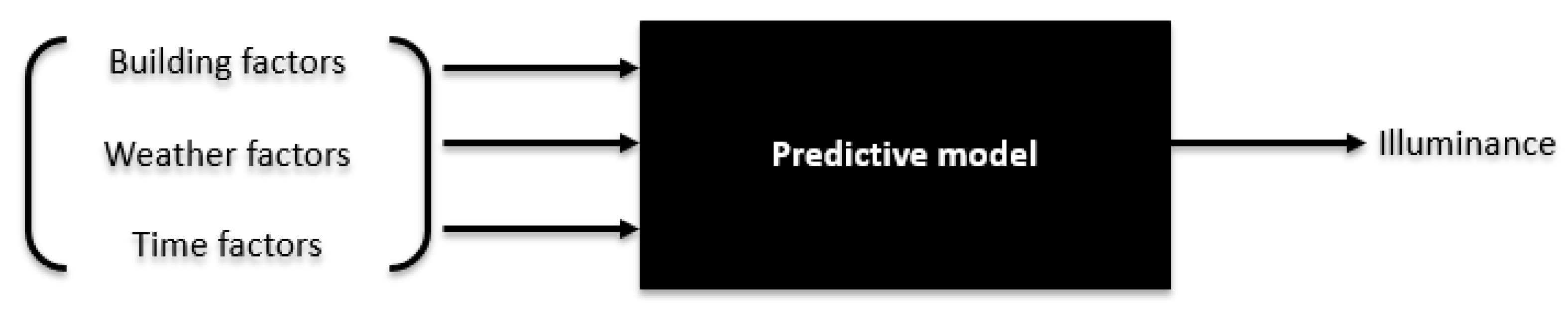
3. Methodology
3.1. Model Parameters
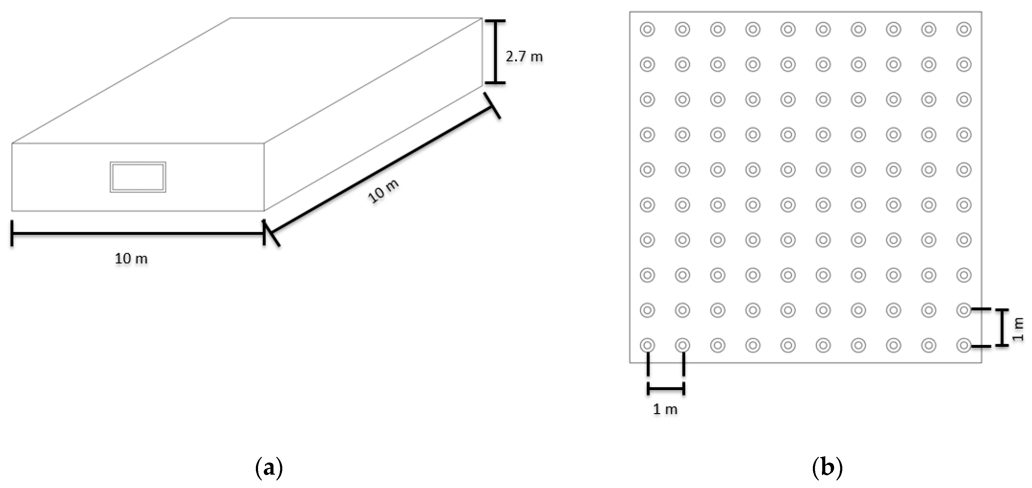
3.2. Data Acquisition (Simulation Design)
3.3. Model Development and Optimization Techniques
3.4. Evaluation of Model Performance
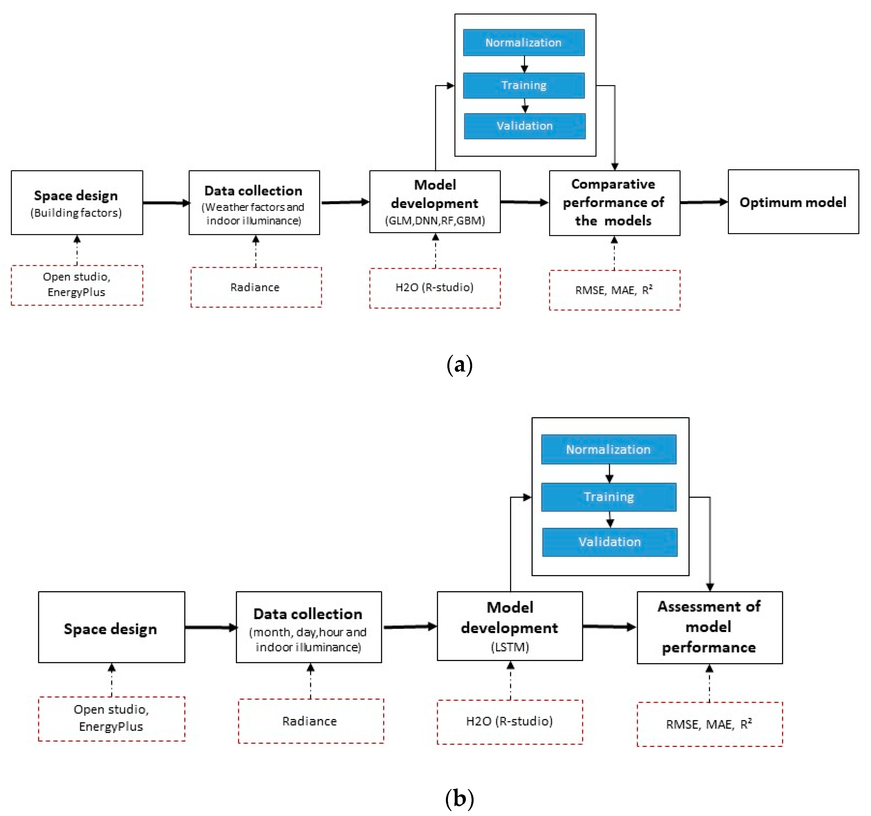
3.5. Study Process
4. Results
4.1. Performance of the Developed Models
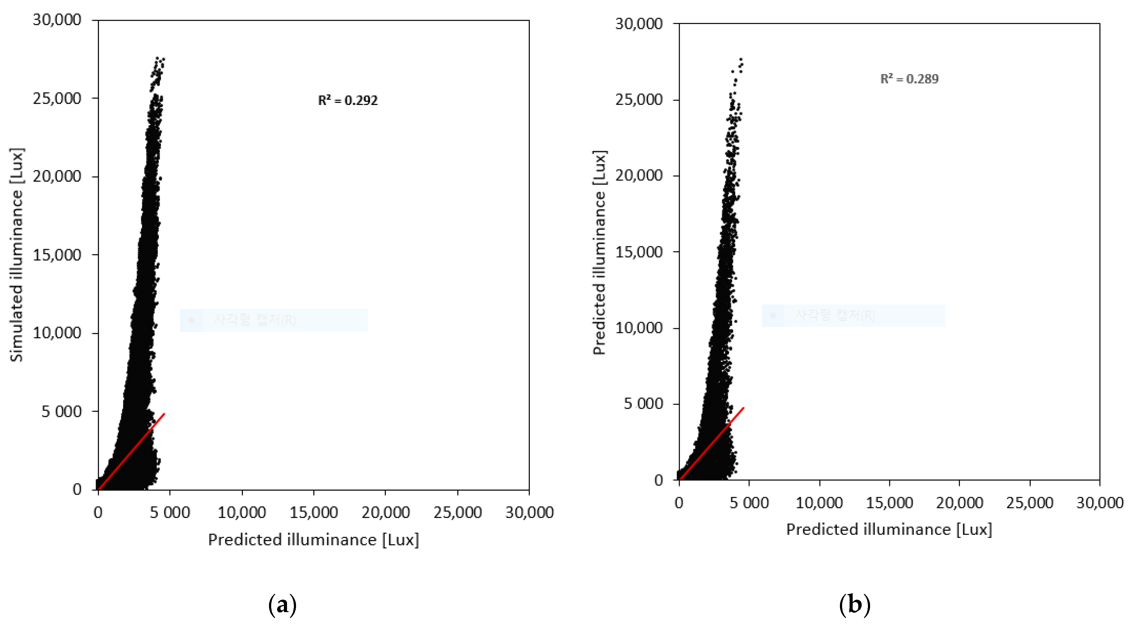
4.1.1. GLM
4.1.2. RF
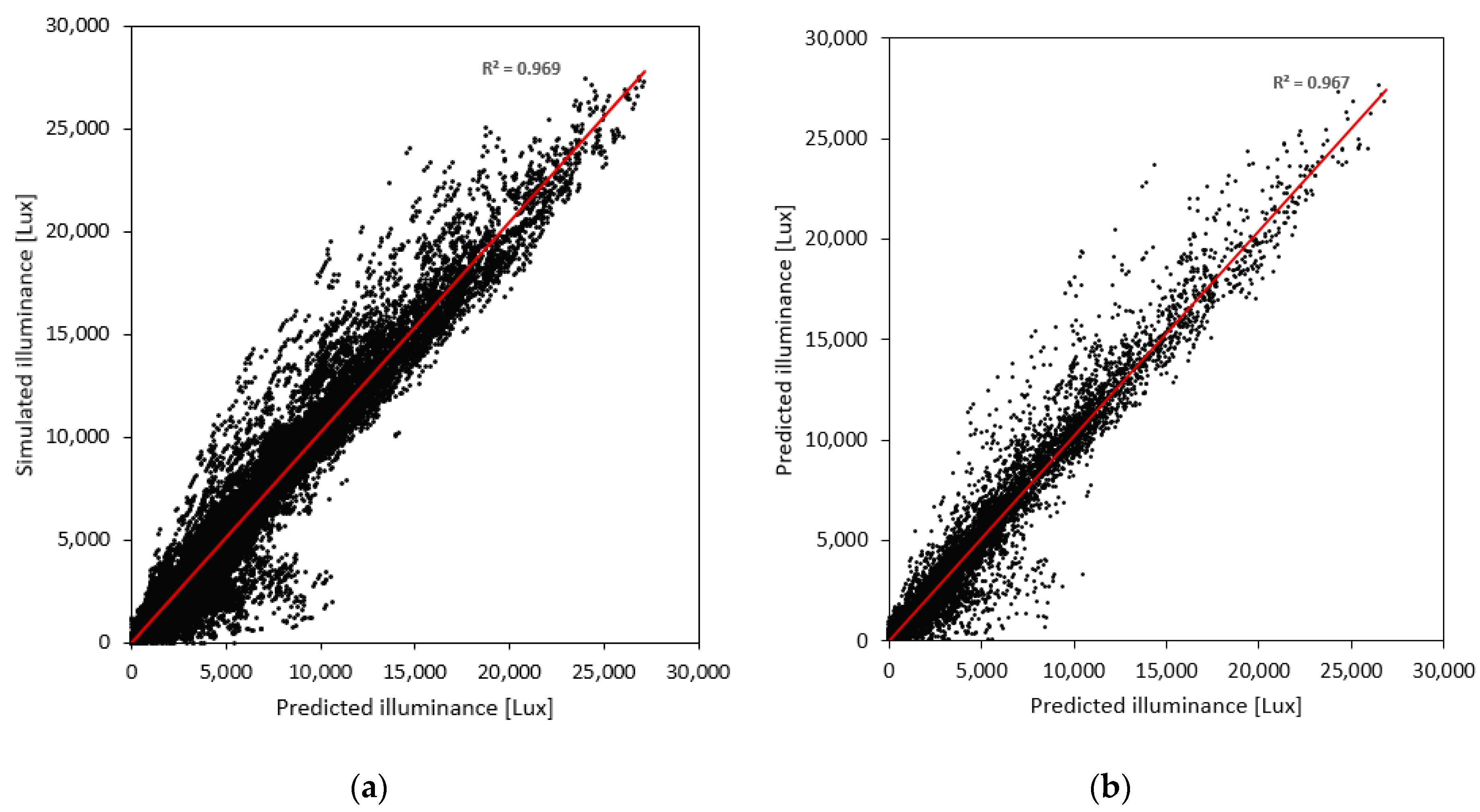
4.1.3. GBM
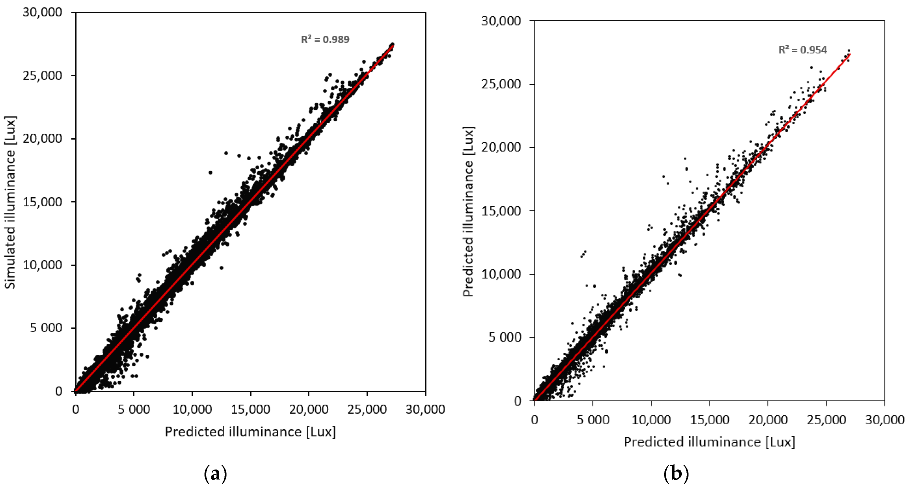
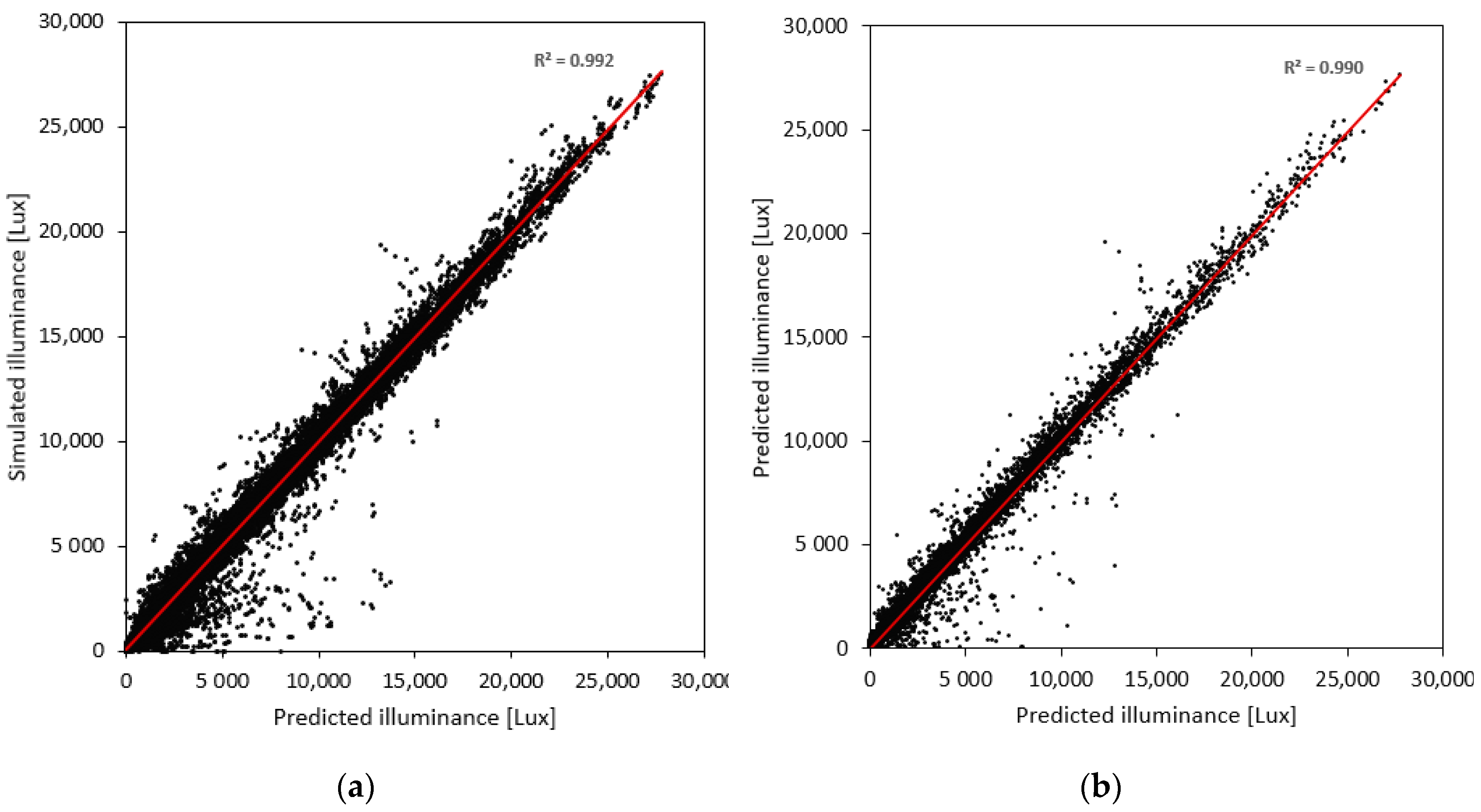
4.1.4. Deep Neural Network (DNN)
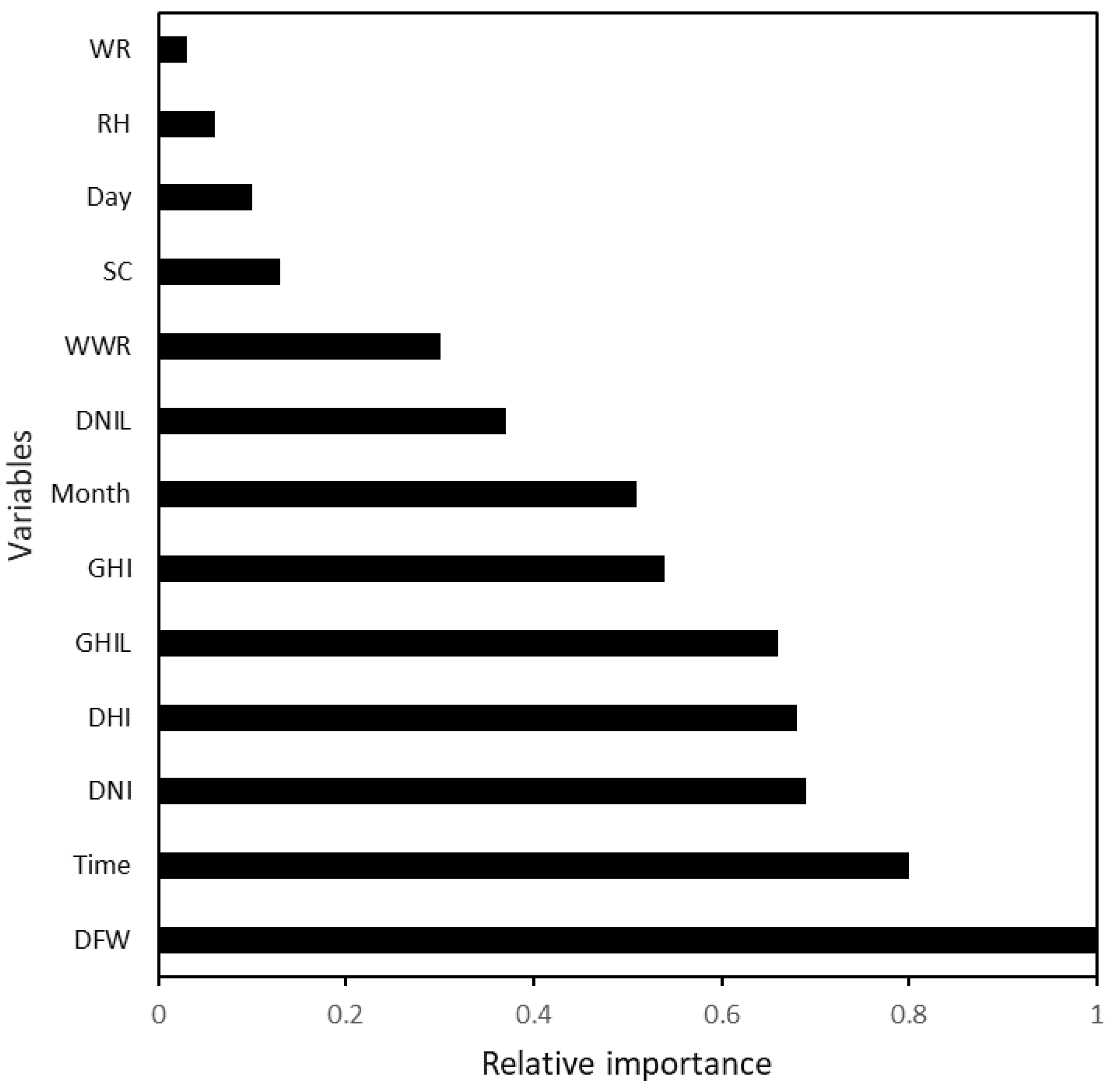
4.2. Relative Importance of the Factors Affecting Daylight Indoor Illuminance
4.3. Comparative Performance of the Developed Models
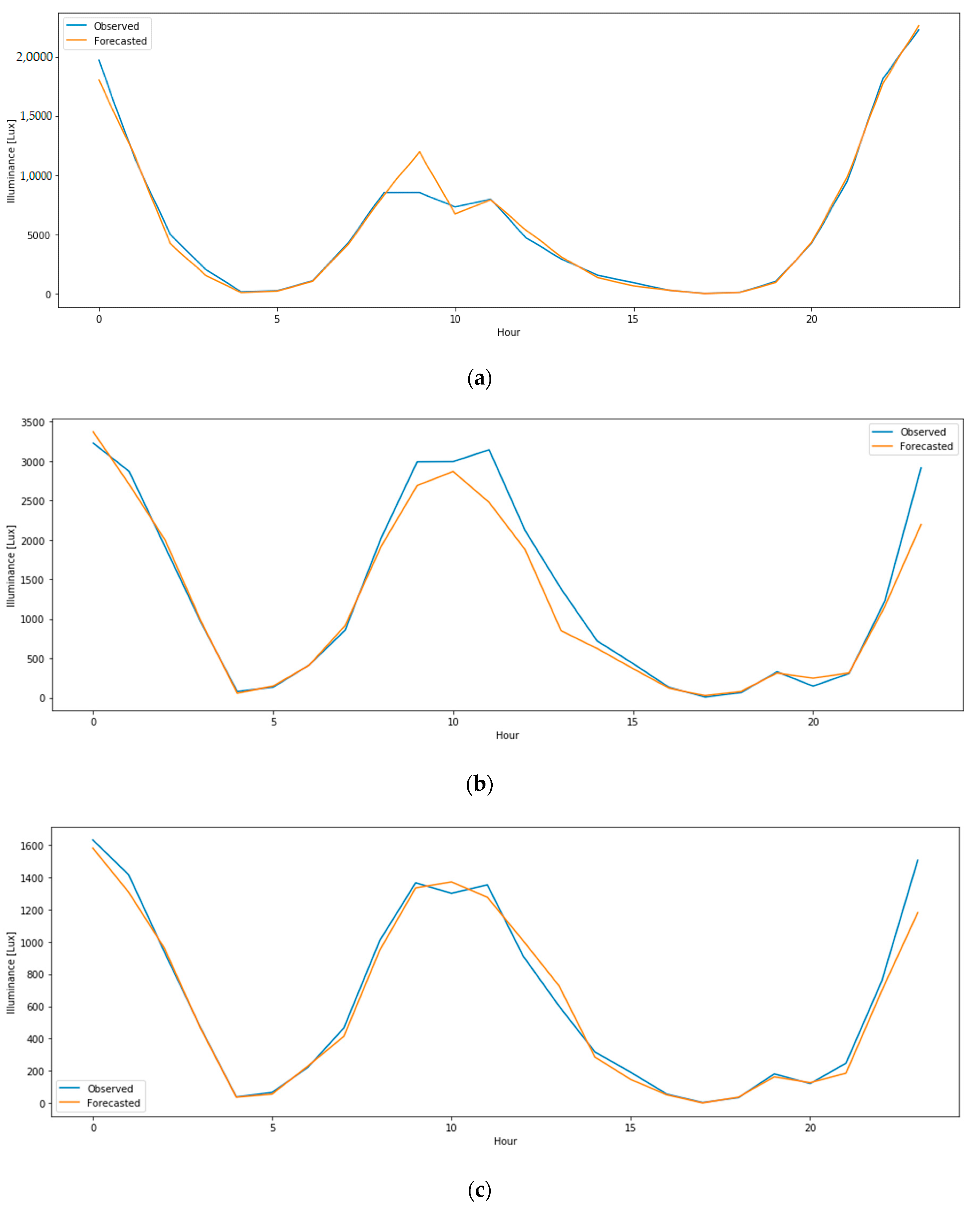
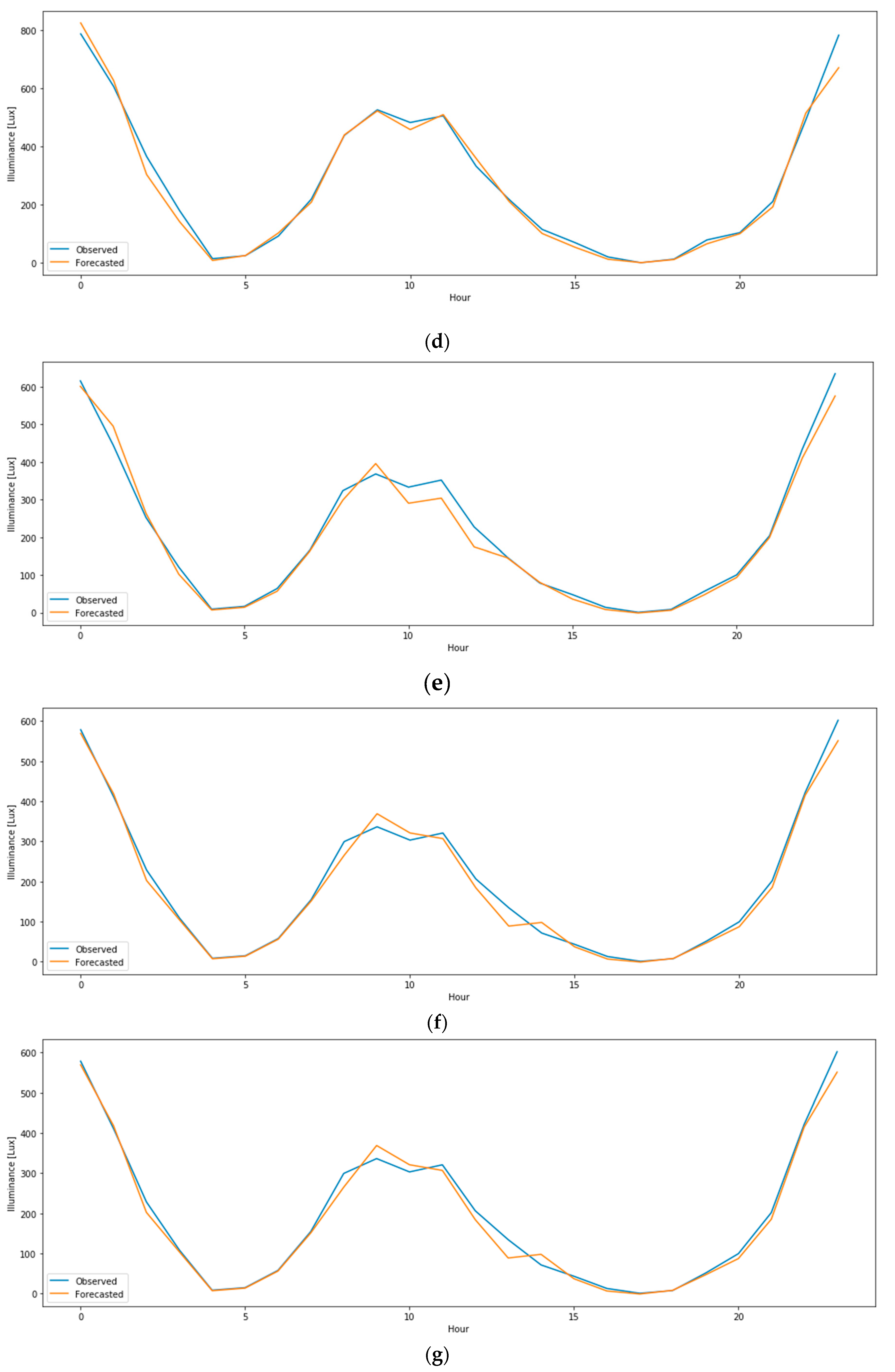
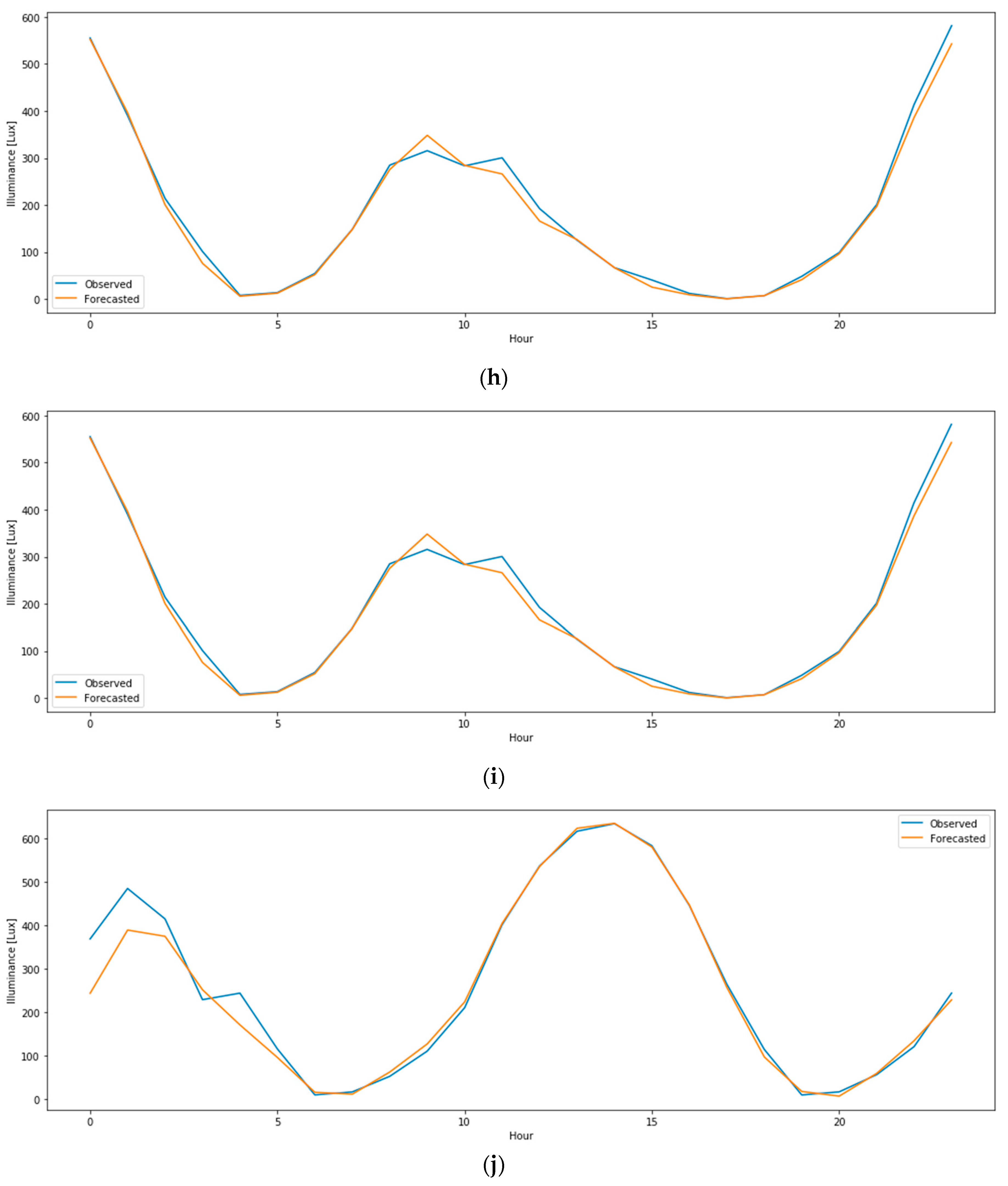
4.4. Forecasting of Daylight Indoor Illuminance Using LSTM
5. Discussion
5.1. Potential Applications of Data-Driven Models in the Daylight Design of Buildings
5.2. Potential Applications of Data-Driven Models in Automated Daylight Control Systems
5.3. Potential Applications in Data-Driven Models in the Preemptive Control of Daylighting
5.4. Optimum Machine Learning Algorithms for the Prediction of Indoor Illuminance Levels
5.5. Limitations and Future Research
6. Conclusions
Author Contributions
Funding
Conflicts of Interest
References
- Yu, X.; Su, Y. Daylight availability assessment and its potential energy saving estimation –A literature review. Renew. Sustain. Energy Rev. 2015, 52, 494–503. [Google Scholar] [CrossRef]
- Shishegar, N.; Boubekri, M. Natural Light and Productivity: Analyzing the Impacts of Daylighting on Students’ and Workers’ Health and Alertness. IJACEBS 2016, 3. [Google Scholar] [CrossRef]
- Chen, X.; Zhang, X.; Du, J. Exploring the effects of daylight and glazing types on self-reported satisfactions and performances: A pilot investigation in an office. Archit. Sci. Rev. 2019, 62, 338–353. [Google Scholar] [CrossRef]
- Bellia, L.; Bisegna, F.; Spada, G. Lighting in indoor environments: Visual and non-visual effects of light sources with different spectral power distributions. Build. Environ. 2011, 46, 1984–1992. [Google Scholar] [CrossRef]
- Ayoub, M. 100 Years of daylighting: A chronological review of daylight prediction and calculation methods. Sol. Energy 2019, 194, 360–390. [Google Scholar] [CrossRef]
- Boccia, O.; Zazzini, P. Daylight in buildings equipped with traditional or innovative sources: A critical analysis on the use of the scale model approach. Energy Build. 2015, 86, 376–393. [Google Scholar] [CrossRef]
- Jakica, N. State-of-the-art review of solar design tools and methods for assessing daylighting and solar potential for building-integrated photovoltaics. Renew. Sustain. Energy Rev. 2018, 81, 1296–1328. [Google Scholar] [CrossRef]
- Ochoa, C.E.; Aries, M.B.C.; Hensen, J.L.M. State of the art in lighting simulation for building science: A literature review. J. Build. Perform. Simul. 2012, 5, 209–233. [Google Scholar] [CrossRef]
- Lorenz, C.L.; Packianather, M.; Spaeth, A.B.; De Souza, C.B. Artificial neural network-based modelling for daylight evaluations. In Proceedings of the 2018 Symposium on Simulation for Architecture and Urban Design (SimAUD 2018), San Diego, CA, USA, June 2018; Society for Modeling and Simulation International (SCS): Delft, The Netherlands, 2018. [Google Scholar]
- Zomorodian, Z.S.; Tahsildoost, M. Assessing the effectiveness of dynamic metrics in predicting daylight availability and visual comfort in classrooms. Renew. Energy 2019, 134, 669–680. [Google Scholar] [CrossRef]
- Jordan, M.I.; Mitchell, T.M. Machine learning: Trends, perspectives, and prospects. Science 2015, 349, 255–260. [Google Scholar] [CrossRef]
- Kazanasmaz, T.; Günaydin, M.; Binol, S. Artificial neural networks to predict daylight illuminance in office buildings. Build. Environ. 2009, 44, 1751–1757. [Google Scholar] [CrossRef]
- Ahmad, M.W.; Hippolyte, J.-L.; Mourshed, M.; Rezgui, Y. Random forests and artificial neural network for predicting daylight Illuminance and energy consumption. In Proceedings of the 15th Conference of International Building Performance Simulation Association, San Francisco, CA, USA, March 2018. [Google Scholar]
- Zhou, S.; Liu, D. Prediction of daylighting and energy performance using artificial neural network and support vector machine. Am. J. Civ. Eng. Archit. 2015, 3, 1–8. [Google Scholar]
- Waheeb, W.; Ghazali, R.; Ismail, L.H.; Kadir, A.A. Modelling and forecasting indoor illumination time series data from light pipe system. In International Conference of Reliable Information and Communication Technology; Springer: Cham, Switzerland, 2018; pp. 57–64. [Google Scholar]
- Kurian, C.P.; George, V.I.; Bhat, J.; Aithal, R.S. ANFIS model for the time series prediction of interior daylight illuminance. Int. J. Artif. Intell. Mach. Learn. 2006, 6, 35–40. [Google Scholar]
- Mathew Biju, S. Analyzing the predictive capacity of various machine learning algorithms. IJET 2018, 7, 266. [Google Scholar] [CrossRef]
- Ibrahim, I.A.; Khatib, T. A novel hybrid model for hourly global solar radiation prediction using random forests technique and firefly algorithm. Energy Convers. Manag. 2017, 138, 413–425. [Google Scholar] [CrossRef]
- Biau, G.; Scornet, E. A random forest guided tour. TEST 2016, 25, 197–227. [Google Scholar] [CrossRef]
- Hayes, M.M.; Miller, S.N.; Murphy, M.A. High-resolution landcover classification using Random Forest. Remote Sens. Lett. 2014, 5, 112–121. [Google Scholar] [CrossRef]
- Svetnik, V.; Liaw, A.; Tong, C.; Culberson, J.C.; Sheridan, R.P.; Feuston, B.P. Random forest: A classification and regression tool for compound classification and QSAR modeling. J. Chem. Inf. Comput. Sci. 2003, 43, 1947–1958. [Google Scholar] [CrossRef]
- Qi, C.; Chen, Q.; Fourie, A.; Zhang, Q. An intelligent modelling framework for mechanical properties of cemented paste backfill. Miner. Eng. 2018, 123, 16–27. [Google Scholar] [CrossRef]
- Aljarah, I.; Faris, H.; Mirjalili, S. Optimizing connection weights in neural networks using the whale optimization algorithm. Soft Comput 2018, 22, 1–15. [Google Scholar] [CrossRef]
- Shanmuganathan, S. Artificial Neural Network Modelling: An Introduction. In Artificial Neural Network Modelling; Studies in Computational Intelligence; Shanmuganathan, S., Samarasinghe, S., Eds.; Springer International Publishing: Cham, Switzerland, 2016; Volume 628, pp. 1–14. ISBN 978-3-319-28493-4. [Google Scholar]
- Suzuki, K. (Ed.) Artificial Neural Networks: Methodological Advances and Biomedical Applications; BoD–Books on Demand: Norderstedt, Germany, 2011. [Google Scholar]
- Ermis, K.; Erek, A.; Dincer, I. Heat transfer analysis of phase change process in a finned-tube thermal energy storage system using artificial neural network. Int. J. Heat Mass Tran. 2007, 50, 3163–3175. [Google Scholar] [CrossRef]
- Sak, H.; Senior, A.W.; Beaufays, F. Long short-term memory recurrent neural network architectures for large scale acoustic modeling. arXiv 2014, arXiv:1402.1128. [Google Scholar]
- Kong, W.; Dong, Z.Y.; Jia, Y.; Hill, D.J.; Xu, Y.; Zhang, Y. Short-Term Residential Load Forecasting Based on LSTM Recurrent Neural Network. IEEE Trans. Smart Grid 2019, 10, 841–851. [Google Scholar] [CrossRef]
- Weninger, F.; Erdogan, H.; Watanabe, S.; Vincent, E.; Le Roux, J.; Hershey, J.R.; Schuller, B. Speech enhancement with LSTM recurrent neural networks and its application to noise-Robust ASR. In Latent Variable Analysis and Signal Separation; Lecture Notes in Computer Science; Vincent, E., Yeredor, A., Koldovský, Z., Tichavský, P., Eds.; Springer International Publishing: Cham, Switzerland, 2015; Volume 9237, pp. 91–99. ISBN 978-3-319-22481-7. [Google Scholar]
- Crawley, D.B.; Lawrie, L.K.; Winkelmann, F.C.; Buhl, W.F.; Huang, Y.J.; Pedersen, C.O.; Strand, R.K.; Liesen, R.J.; Fisher, D.E.; Witte, M.J.; et al. EnergyPlus: Creating a new-generation building energy simulation program. Energy Build. 2001, 33, 319–331. [Google Scholar] [CrossRef]
- McNeil, A.; Lee, E.S. A validation of the Radiance three-phase simulation method for modelling annual daylight performance of optically complex fenestration systems. J. Build. Perform. Simul. 2013, 6, 24–37. [Google Scholar] [CrossRef]
- Yoon, Y.; Moon, J.W.; Kim, S. Development of annual daylight simulation algorithms for prediction of indoor daylight illuminance. Energy Build. 2016, 118, 1–17. [Google Scholar] [CrossRef]
- Reinhart, C.F.; Andersen, M. Development and validation of a Radiance model for a translucent panel. Energy Build. 2006, 38, 890–904. [Google Scholar] [CrossRef]
- Heaton, J. Introduction to Neural Networks with Java; Heaton Research, Inc.: St. Louis, MO, USA, 2008. [Google Scholar]
- Hecht-Nielsen, R. Theory of the Backpropagation Neural Network**Based on “nonindent” by Robert Hecht-Nielsen, which appeared in Proceedings of the International Joint Conference on Neural Networks 1, 593–611, June 1989. © 1989 IEEE. In Neural Networks for Perception; Elsevier: Amsterdam, The Netherlands, 1992; pp. 65–93. ISBN 978-0-12-741252-8. [Google Scholar]
- Schmidhuber, J. Deep learning in neural networks: An overview. Neural Netw. 2015, 61, 85–117. [Google Scholar] [CrossRef]
- Willmott, C.; Matsuura, K. Advantages of the mean absolute error (MAE) over the root mean square error (RMSE) in assessing average model performance. Clim. Res. 2005, 30, 79–82. [Google Scholar] [CrossRef]
- Chai, T.; Draxler, R.R. Root mean square error (RMSE) or mean absolute error (MAE)?–Arguments against avoiding RMSE in the literature. Geosci. Model Dev. 2014, 7, 1247–1250. [Google Scholar] [CrossRef]
- Garson, G.D. Interpreting Neural-Network Connection Weights; AI Expert, Miller Freeman, Inc: San Francisco, CA, USA, 1991; Volume 6, pp. 46–51. [Google Scholar]
- Jang, J.-S.R. ANFIS: Adaptive-network-based fuzzy inference system. IEEE Trans. Syst. Man Cybern. 1993, 23, 665–685. [Google Scholar] [CrossRef]
- Mukherjee, S.; Birru, D.; Cavalcanti, D.; Shen, E.; Patel, M.; Wen, Y.J.; Das, S. Closed loop integrated lighting and daylighting control for low energy buildings. In Proceedings of the 2010 ACEEE 2010, Summer Study on Energy Efficiency in Buildings, California, CA, USA, 15–20 August 2010; pp. 252–269. [Google Scholar]
- Gamboa, J.C.B. Deep Learning for Time-Series Analysis. arXiv 2017, arXiv:1701.01887. [Google Scholar]
- Athey, S.; Imbens, G.W. Machine Learning Methods for Estimating Heterogeneous Causal Effects. Stat 2015, 1050, 1–26. [Google Scholar]


| Parameter | Min | Max |
|---|---|---|
| WWR [%] | 20 | 60 |
| WR [%] | 20 | 60 |
| DFW [m] | 0 | 9 |
| GHI [w/m2] | 0 | 992 |
| DNI [w/m2] | 0 | 970 |
| DHI [w/m2] | 0 | 970 |
| GHIL [Lux] | 0 | 121,265 |
| DNIL [Lux] | 0 | 97,695 |
| RH [%] | 10 | 98 |
| SC [%] | 0 | 100 |
| Month | 1 | 12 |
| Day | 1 | 365 |
| Time [hours] | 6 | 20 |
| Illuminance [Lux] | 0 | 27,580 |
| RF | GBM | DNN | LSTM | |
|---|---|---|---|---|
| Number of hidden layers | n/a | n/a | 5 | 3 |
| Number of neurons in the hidden layer | n/a | n/a | 29 | 25 |
| Number of trees | 10 | 12 | n/a | n/a |
| Epochs | n/a | n/a | 1000 | 1000 |
| Learning rate | n/a | 0.1 | 0.01 | 0.01 |
| Loss function | MSE | LS | RMSE | RMSE |
| Optimizer | n/a | n/a | Adam | Adam |
| Maximum features | Auto | Auto | n/a | n/a |
| Activation function | n/a | n/a | ReLU | ReLU |
| Sample rate | 0.8 | 0.8 | n/a | n/a |
| Dataset | N | Range | Minimum | Maximum | Mean | Std. Deviation |
|---|---|---|---|---|---|---|
| Training | 337,256 | 27,492.60 | 0.00 | 27,492.60 | 794.88 | 2233.90 |
| Validation | 83,989 | 27,580.40 | 0.00 | 27,580.40 | 784.84 | 2214.13 |
| Number of Trees | Training Dataset | Validation Dataset | ||||
|---|---|---|---|---|---|---|
| RMSE | MAE | R2 | RMSE | MAE | R2 | |
| 2 | 328.328 | 64.333 | 0.978 | 255.553 | 56.714 | 0.986 |
| 4 | 277.693 | 59.137 | 0.984 | 184.811 | 47.802 | 0.983 |
| 6 | 262.218 | 56.401 | 0.986 | 171.599 | 44.934 | 0.983 |
| 8 | 262.218 | 53.383 | 0.988 | 161.833 | 42.268 | 0.984 |
| 10 | 228.256 | 52.387 | 0.989 | 155.564 | 41.713 | 0.954 |
| Number of Trees | Training Dataset | Validation Dataset | ||||
|---|---|---|---|---|---|---|
| RMSE | MAE | R2 | RMSE | MAE | R2 | |
| 10 | 2072.213 | 934.812 | 0.139 | 2054.344 | 929.155 | 0.139 |
| 50 | 1573.895 | 682.162 | 0.503 | 1562.909 | 679.473 | 0.501 |
| 100 | 1168.233 | 487.698 | 0.503 | 1562.909 | 486.725 | 0.724 |
| 500 | 461.895 | 144.498 | 0.957 | 470.002 | 144.967 | 0.954 |
| 1000 | 393.956 | 120.943 | 0.969 | 403.989 | 122.190 | 0.967 |
| Number of Trees | Training Dataset | Validation Dataset | ||||
|---|---|---|---|---|---|---|
| RMSE | MAE | R2 | RMSE | MAE | R2 | |
| 1 | 471.389 | 222.267 | 0.955 | 477.517 | 224.106 | 0.953 |
| 2 | 241.282 | 86.860 | 0.988 | 252.232 | 88.079 | 0.987 |
| 3 | 207.614 | 79.638 | 0.991 | 228.320 | 81.580 | 0.989 |
| 4 | 195.301 | 67.558 | 0.992 | 211.443 | 69.166 | 0.990 |
| 5 | 199.274 | 69.136 | 0.991 | 222.791 | 71.893 | 0.990 |
| Training Dataset | Validation Dataset | |||||
|---|---|---|---|---|---|---|
| RMSE | MAE | R2 | RMSE | MAE | R2 | |
| GLM | 1881.14 | 995.811 | 0.290 | 1868.031 | 992.051 | 0.288 |
| RF | 228.256 | 52.387 | 0.989 | 470.002 | 144.967 | 0.954 |
| GBM | 393.956 | 120.943 | 0.969 | 403.989 | 122.190 | 0.967 |
| DNN | 199.274 | 69.136 | 0.992 | 222.791 | 71.893 | 0.990 |
| Training Dataset | Validation Dataset | |||||
|---|---|---|---|---|---|---|
| RMSE | MAE | R2 | RMSE | MAE | R2 | |
| GLM | 1915.851 | 987.344 | 0.264 | 1900.645 | 982.359 | 0.263 |
| RF | 1237.218 | 390.242 | 0.695 | 1061.408 | 340.497 | 0.774 |
| GBM | 1074.865 | 347.405 | 0.768 | 1081.591 | 346.671 | 0.761 |
| DNN | 1042.133 | 346.390 | 0.782 | 1043.933 | 344.732 | 0.777 |
| Model | All Variables | Important Variables |
|---|---|---|
| GLM | 0.64 | 0.15 |
| RF | 150 | 113 |
| GBM | 129 | 107 |
| DNN | 204 | 143 |
© 2020 by the authors. Licensee MDPI, Basel, Switzerland. This article is an open access article distributed under the terms and conditions of the Creative Commons Attribution (CC BY) license (http://creativecommons.org/licenses/by/4.0/).
Share and Cite
Ngarambe, J.; Irakoze, A.; Yun, G.Y.; Kim, G. Comparative Performance of Machine Learning Algorithms in the Prediction of Indoor Daylight Illuminances. Sustainability 2020, 12, 4471. https://doi.org/10.3390/su12114471
Ngarambe J, Irakoze A, Yun GY, Kim G. Comparative Performance of Machine Learning Algorithms in the Prediction of Indoor Daylight Illuminances. Sustainability. 2020; 12(11):4471. https://doi.org/10.3390/su12114471
Chicago/Turabian StyleNgarambe, Jack, Amina Irakoze, Geun Young Yun, and Gon Kim. 2020. "Comparative Performance of Machine Learning Algorithms in the Prediction of Indoor Daylight Illuminances" Sustainability 12, no. 11: 4471. https://doi.org/10.3390/su12114471
APA StyleNgarambe, J., Irakoze, A., Yun, G. Y., & Kim, G. (2020). Comparative Performance of Machine Learning Algorithms in the Prediction of Indoor Daylight Illuminances. Sustainability, 12(11), 4471. https://doi.org/10.3390/su12114471