A Predictive Analysis of China’s CO₂ Emissions and OFDI with a Nonlinear Fractional-Order Grey Multivariable Model

Abstract

Since the implementation of the Belt and Road Initiative, China’s total amount of outward foreign direct investment (OFDI) has increased each year and this has caused its relationship with carbon emissions (CO₂e) to receive great attention recently. Forecasting China’s CO₂e accurately by considering the impact of OFDI is important since the government can use it to formulate an appropriate emissions plan to fulfill its carbon reduction commitments. Because the relationship between OFDI and CO₂e has nonlinear characteristics, a nonlinear grey multivariable model with fractional-order accumulation (NFGM(1,N)) was proposed in this study. To enhance the prediction accuracy, an optimization process was used to determine the parameters. The outcomes of the variable fractional order showed that fractional-order accumulation can better extract the grey information hidden in the original data, which confirmed the principle of new information priority. The result of the power coefficient indicated a nonlinear relationship between the CO₂e and OFDI. Based on the prediction performance, the prediction accuracy of the NFGM(1,N) model was proven to be superior to those of the ARMA model, linear regression model, the GM(1,1), GM(1,N), and FGM(1,N) models. The empirical results also revealed that OFDI increased the CO₂e in China. The relationship between the CO₂e and OFDI exhibits a U-shaped development based on further predictions for the 2018–2030 period. Finally, some suggestions for long-term CO₂e reduction plans were provided in this paper.

1. Introduction

In recent years, excessive carbon dioxide emissions (CO₂e) have caused a series of severe environmental problems, such as global warming, the melting of glaciers, and the frequent occurrence of extreme weather, and they also have had a harmful influence on human health. For those reasons, countries around the world have put their efforts into CO₂e reduction and have committed to setting emissions reduction goals. China, as the largest developing country with the largest CO₂e in the world [1], promised at the UN Climate Change Summit in 2009 (COP15) that the CO₂e per unit of GDP will be reduced by 40%–45% at the end of 2020 compared to 2005. Moreover, at the Paris Climate Change Conference in 2015 (COP21), China further committed to reduce its CO₂e by 60%–65% by 2030 compared to 2005. Therefore, it is meaningful for the government to accurately forecast China’s CO₂e to enable it to comprehend the trend of emissions and to realize its CO₂e reduction commitment.

The issues regarding the impact factor analysis and prediction of CO₂e have received great attention from both academics and practitioners. Previous studies have found that economic growth, energy consumption, urban population, and research and development (R&D, for details of Nomenclature, refer to “Appendix A”) were important factors affecting CO₂e [2,3], predicted emissions by considering the effects of these factors [4,5,6]. General speaking, reducing CO₂e mainly depends on technological advances, which come from the R&D undertaken and foreign direct investments (FDI) [7,8,9]. In the past few decades, many academics have focused on analyzing the relationship between FDI and CO₂e, and they concluded that inward FDI (IFDI) and outward FDI (OFDI) could affect CO₂e [10,11]. However, compared to IFDI, there are still few studies on the relationship between OFDI and CO₂e, and no complete theoretical system has been generated. The results of previous studies showed that OFDI had an increased or a reduced impact on CO₂e [12,13]. In the context of the uncertain effects, it can be recognized that there is a nonlinear relationship between OFDI and CO₂e [14]. With the implementation of the “go out” strategy, especially the Belt and Road Initiative proposed in 2013, China’s OFDI increased continuously and first surpassed IFDI in 2016, when it reached 216.42 million U.S. dollars. Therefore, in consideration of the upward trend of OFDI, it is essential to analyze the relationship between China’s CO₂e and OFDI, and forecast emissions by evaluating the effect of OFDI.

Due to the increasing trend of OFDI, forecasting China’s CO₂e by considering the impact of OFDI helps to improve the prediction accuracy, which also makes the grey multivariable GM(1,N) model stand out from the numerous grey models. The GM(1,N) model, which was proposed by Deng [15], is a prediction model with one system characteristics variable and N-1 relevant variables. More specifically, the GM(1,N) model is a typical causal prediction model because it takes full account of the effect of the relevant factors on the system behavior change in the whole modeling process [16]. At present, the traditional GM(1,N) model uses the first-order accumulated generating operation (1-AGO) to generate a sequence; however, 1-AGO is not consistent with the principle of the new information priority in the grey system theory. Therefore, Wu et al. [17] proposed fractional-order accumulation to give separate weights to older and newer data, which had been combined with the GM(1,1) and GM(1,N) models [18,19,20]. In this study, the fractional-order accumulated generating operation is introduced to the traditional GM(1,N) model (the FGM(1,N) model) to further improve the prediction accuracy. Furthermore, the GM(1,N) is a linear prediction model; in other words, with this model it is not appropriate to reflect the nonlinear relationship between system characteristics variable and relevant variables in reality [21]. Referring to the nonlinear grey model used in previous studies [22,23], this study proposes the nonlinear fractional grey multivariable model, abbreviated as the NFGM(1,N), to predict China’s CO₂e by considering the nonlinear relationship between the OFDI and emissions. The fractional order, power, and the coefficients in modeling, are the crucial issues which influence the prediction accuracy of the proposed model. Therefore, finally, this study applies the optimization algorithm to determine the values of the parameters.

The rest of this paper is organized as follows. Section 2 is a review of previous related literature. The proposed nonlinear fractional grey multivariable model is presented in Section 3. Section 4 predicts the CO₂e in China by considering the effect of the OFDI. The conclusions are listed in Section 5.

2. Literature Review

2.1. Relationship between OFDI and Carbon Emissions

Compared with the studies of the relationship between IFDI and CO₂e in host countries, there has been little research concentrating on the effects of OFDI from the home country’s perspective [24]. Among the existing studies, on the one hand, most of them concluded that the OFDI had an impact on reducing CO₂e. Liu and Gong [25] and Jiang et al. [14] concluded that an increase in OFDI had a positive effect on emissions reduction. Nie and Liu [24] used provincial panel data to analyze the effect of OFDI on CO₂e and found that although OFDI was beneficial to reduce the emissions, it was restricted by the threshold effect of urbanization. Long and Zhou [26] mentioned that OFDI had a positive effect on carbon productivity because of the reverse technology spillover effect. More specifically, they found that the carbon productivity increased by 0.37% for each 10% of the increases in the OFDI reverse technology spillover effect, but the effect was different in different regions. On the other hand, several studies hold the opposite view; that is, that OFDI would increase the CO₂e in the home country. By using an applied panel threshold model, Yang and Sun [27] found that OFDI aggravated environmental pollution. Liu and Li [13] used provincial panel data to examine China’s home country effect on CO₂e and found that the per capita CO₂e increases by 0.012% for each 1% increase in OFDI, but there were regional differences in this result.

The reasons for the uncertain relationship between OFDI and CO₂e can be summarized as follows. First, based on Kojima’s theory of marginal industry expansion, one country prefers to transfer its marginal industries with high energy consumption and emissions to the other country, which causes the CO₂e to decline in the home country due to the emissions transference effect. Second, as Buckley et al. [28] stated, China’s OFDI was motivated by resource seeking; thus, the resource-intensive industries were transferred by OFDI, which reduced the CO₂e in the home country [25]. However, as stated in the study of Liu and Li [13], China’s OFDI was not dominated by the industries with high emissions, so the emissions transference motivation was not clear. Third, owing to the reverse spillover effects from the resources and technologies backflow, the energy-related technical levels in the home country were enhanced, thereby reducing the CO₂e [29,30]. However, the technological spillover effect on China’s emission reduction will be varied because of the differences in economic development and absorptive capacity in different regions.

According to the reviews above, the general conclusion can be drawn that OFDI has a significant impact on CO₂e, but the effect is uncertain. Furthermore, the positive or negative effect of OFDI on CO₂e indicates that there is a nonlinear relationship between these two variables [31,32].

2.2. China’s CO₂e Forecasting Using Grey Model

The widely used prediction models can be roughly categorized into two groups: econometrics methods, including regression models and time series analyses, and intelligence computational technologies. However, knowing the sample distribution and having a large amount of data are the bases of accurate predictions with econometrics methods. Successful intelligence computational technology also needs a large amount of training data [17]. Under these circumstances, the grey model, which works well with an uncertain system, small sample size, poor information, and without the need to make any statistical assumptions, has drawn considerable attention. Grey models have been successfully applied in several disciplines and achieved great performance [20,33,34,35].

A grey prediction model and the improved versions of it have often been applied to the issues related to China’s CO₂e forecasting. Overall, the grey models used can be divided into univariable and multivariable models; these are represented by the GM(1,1) and GM(1,N) model, respectively. To examine whether China can achieve its peak emissions commitment by 2030, Li et al. [36] applied the traditional GM(1,1) model to predict China’s CO₂e. Meng et al. [37] predicted the energy-related CO₂ in China using a small-sample hybrid model that combined the GM(1,1) model with a linear model, and they estimated the parameters by using a non-constrained optimization equation. Considering the nonlinear feature of a sequence, Pao et al. [38] forecast China’s CO₂e by the nonlinear grey Bernoulli NGBM(1,1) model, and they used a combined iterative numerical method as an optimization method to improve the prediction accuracy. Wu et al. [39] applied a conformable fractional non-homogeneous grey model to predict the CO₂e in the BRICS (Brazil, Russia, India, China, and South Africa) countries. However, because the GM(1,1) model only reflects the sequence response to time, many studies applied the GM(1,N) model to predict China’s CO₂e while considering the effects of relevant factors [40]. Wu et al. [5] predicted the CO₂e in the BRICS countries by using GM(1,N) with an opposite-direction accumulated generating operator. Wang and Ye [21], Wang and Li [23] applied a nonlinear grey multivariable model and derived the non-equigap grey Verhulst model to predict the CO₂e in combination with optimization algorithms.

A review of the literature shows that the fractional-order accumulative generation operation has been combined with the grey model and achieved great prediction performance. The introduction of fractional order only changes the way the sequence accumulation generates and does not change the linear feature of the GM(1,N) model, so it is still inappropriate to reflect the nonlinear relationship between the system variables and relevant variables. Therefore, this study proposed the NFGM(1,N) model and introduced the power model to the FGM(1,N) model to predict China’s CO₂e by reflecting the nonlinear effect of OFDI.

3. Methodology

The NFGM(1,N) model is an extension of the FGM(1,N) model and reflects the nonlinear relationship between the dependent variable and independent variables by introducing the power model to the FGM(1,N) model. The processes of the proposed NFGM(1,N) model and the determination of the parameters are demonstrated in this section. For details of traditional GM(1,N) model, refer to “Appendix B”. A numerical example is then used to verify the validity of the NFGM(1,N) model.

3.1. Nonlinear Fractional Grey Multivariable Model

The computational steps to construct an NFGM(1,N) model are demonstrated as follows.

Step 1: Present the data sequences. The system characteristics sequence $X_1^{(0)}=\left(x_1^{(0)}(1),x_1^{(0)}(2),\dots ,x_1^{(0)}(n)\right)$ and relevant factors sequence $X_i^{(0)}=\left(x_i^{(0)}(1),x_i^{(0)}(2),\dots ,x_i^{(0)}(n)\right)$ are presented, where $i=2,3,\dots ,N$.

Step 2: Perform the accumulated generating operation. The accumulative sequence $X_i^{(r_i)}=\left(x_i^{(r_i)}(1),x_i^{(r_i)}(2),\dots ,x_i^{(r_i)}(n)\right)$ can be obtained from $X_i^{(0)}$ by the r_i-order accumulated generating operation (r_i-AGO) as follows:

$$x_i^{(r_i)}={\displaystyle \sum _{j=1}^k\left(\begin{array}{c}k-j+r_i-1\\ k-j\end{array}\right)x_i^{(0)}(j),k=1,2,\dots ,n}$$

(1)

where $\left(\begin{array}{c}k-j+r_i-1\\ k-j\end{array}\right)=\frac{(k-j+r_i-1)(k-j+r_i-2)\dots (r_i+1)r_i}{(k-j)!}$. Based on the study of Wu et al. [41], r should be taken in the interval (0,1).

Step 3: Construct the NFGM(1,N) model. Drawing on the concept from the GM(1,1) model, a grey control parameter term u is added to the model. Therefore, the NFGM(1,N) model is given as

$$\left(x_1^{(r_i)}(k)-x_1^{(r_i)}(k-1)\right)+a{z}_1^{(r_i)}(k)={\displaystyle \sum _{i=2}^n{b}_i{\left(x_i^{(r_i)}(k)\right)}^{{\gamma }_i}}+u$$

(2)

where a, b_i, and u are the coefficients of the modeling, which represent the development term, the driving coefficients, and grey control parameter, respectively. Moreover, r_i and γ_i are the order of the fractional for different variables and the power, respectively. The NFGM(1,N) model reverts to the FGM(1,N) model when γ_i = 1, and it reverts to the traditional GM(1,N) model when r_i = 1 and γ_i = 1.

Step 4: Estimate the coefficients. The parameters a, b_i, and u can be estimated by using the OLS method

$${\left[a,b_i,u\right]}^T={(B^{T}B)}^{-1}{B}^{T}Y$$

(3)

where

$$B=\left[\begin{array}{ccccc}-z_1^{(r_1)}(2)& {\left(x_2^{(r_2)}(2)\right)}^{{\gamma }_2}& \cdots & {\left(x_N^{(r_2)}(2)\right)}^{{\gamma }_N}& 1\\ -z_1^{(r_1)}(3)& {\left(x_2^{(r_2)}(3)\right)}^{{\gamma }_2}& \cdots & {\left(x_N^{(r_2)}(3)\right)}^{{\gamma }_N}& 1\\ ⋮& ⋮& \ddots & ⋮& 1\\ -z_1^{(r_1)}(n)& {\left(x_2^{(r_2)}(n)\right)}^{{\gamma }_2}& \cdots & {\left(x_N^{(r_2)}(n)\right)}^{{\gamma }_N}& 1\end{array}\right],Y=\left[\begin{array}{c}{x}_1^{(r_1)}(2)-x_1^{(r_1)}(1)\\ x_1^{(r_1)}(3)-x_1^{(r_1)}(2)\\ ⋮\\ x_1^{(r_1)}(n)-x_1^{(r_1)}(n-1)\end{array}\right]$$

(4)

where the background values of the system characteristics variable $z_1^{(r_i)}$ are calculated by an adjoining mean generated sequence as follows:

$$z_1^{(r_1)}(k)=0.5\times \left(x_1^{(r_1)}(k)+x_1^{(r_1)}(k-1)\right)$$

(5)

Then, the time response function can be represented as

$${\widehat{x}}_1^{(r)}(k)=\left[x_1^{(r)}(1)-\frac{1}{a}\left({\displaystyle \sum _{i=2}^n{b}_i{\left(x_i^{(r_i)}(k)\right)}^{{\gamma }_i}+u}\right)\right]e^{-a(k-1)}+\left[\frac{1}{a}\left({\displaystyle \sum _{i=2}^n{b}_i{\left(x_i^{(r_i)}(k)\right)}^{{\gamma }_i}+u}\right)\right]$$

(6)

Step 5: Perform the inverse accumulated generating operation. The r-order inverse fractional accumulation can be defined as

$$x^{(-r)}(k)={\displaystyle \sum _{i=1}^k\left(\begin{array}{c}k-i-r-1\\ k-i\end{array}\right)x^{(0)}(i)}$$

(7)

Therefore, the predicted values ${\widehat{X}}_1^{(0)}$ can be calculated by using the inverse r_i-order accumulated generating operation (r_i-IAGO) as follows:

$${\widehat{x}}_1^{(0)}(k)={\left({\widehat{x}}_1^{(r_i)}(k)\right)}^{(-r_i)}={\displaystyle \sum _{j=1}^k\left(\begin{array}{c}k-j-r_i-1\\ k-j\end{array}\right)}{\widehat{x}}_1^{(r)}(j)-{\displaystyle \sum _{j=1}^{k-1}\left(\begin{array}{c}k-1-j-r_i-1\\ k-1-j\end{array}\right)}{\widehat{x}}_1^{(r)}(j),k=2,3,\dots ,n$$

(8)

where ${\widehat{x}}_1^{(r)}(1)=x_1^{(0)}(1)$.

Step 6: Determine the parameters. From the modeling process, once the parameters r_i and γ_i are determined, the other parameters a, b_i, and u are ascertained. The objective of the optimal value of r_i and γ_i should be to make the proposed model have the highest accuracy with the given sample. Therefore, this study establishes an optimization problem where the objective is to minimize the error of the proposed model by changing the values of r_i and γ_i, and the constraints follow the modeling steps of the proposed model. The mean absolute percentage error (MAPE) is applied to assess the prediction performance. In this study, from the perspective of improving the prediction accuracy, taking the minimum MAPE of the modeling as the target, and the relationship between the parameters of the model as a constraint, the non-linear optimization processes are built as follows:

$$\underset{r_i,{\gamma }_i}{\min }MAPE=\frac{1}{n}{\displaystyle \sum _{k=1}^n\left|\frac{x_1^{(0)}(k)-{\widehat{x}}_1^{(0)}(k)}{x_1^{(0)}(k)}\right|}\times 100\%$$

$$s.t.\{\begin{array}{l}{\left[a,b_i,u\right]}^T={(B^{T}B)}^{-1}{B}^{T}Y\\ {\widehat{x}}_1^{(r)}(k)=\left[x_1^{(r)}(1)-\frac{1}{a}\left({\displaystyle \sum _{i=2}^n{b}_i{\left(x_i^{(r_i)}(k)\right)}^{{\gamma }_i}+u}\right)\right]e^{-a(k-1)}+\left[\frac{1}{a}\left({\displaystyle \sum _{i=2}^n{b}_i{\left(x_i^{(r_i)}(k)\right)}^{{\gamma }_i}+u}\right)\right]\\ {\widehat{x}}_1^{(r)}(1)=x_1^{(0)}(1)\\ {\widehat{x}}_1^{(0)}(k)={\left({\widehat{x}}_1^{(r)}(k)\right)}^{(-r)}={\displaystyle \sum _{j=1}^k\left(\begin{array}{c}k-j-r_i-1\\ k-j\end{array}\right)}{\widehat{x}}_1^{(r)}(j)-{\displaystyle \sum _{j=1}^{k-1}\left(\begin{array}{c}k-1-j-r_i-1\\ k-1-j\end{array}\right)}{\widehat{x}}_1^{(r)}(j),k=2,3,\dots ,n\end{array}$$

The above model can be solved by numerical software programing [42].

3.2. An Illustrative Example

To compare the modeling and prediction accuracy, a numerical example from Zeng’s [43] work is used to verify the validation of the proposed NFGM(1,N) model. The system characteristics behavior sequence is X₁⁽⁰⁾ = (11.4918, 12.2255, 13.3201, 14.5930, 17.3891, 21.0232, 26.4446, 23.5325, 46.5982), and the relevant factor sequence is X₂⁽⁰⁾ = (2.6487, 3.7183, 5.4817, 8.3891, 13.1825, 21.0855, 34.1155, 55.5982, 91.0171). The backward data in the sequence represent the newer information. The first eight data are used for model fitting, and the ninth datum is used for ex-post testing. The econometric model, including the autoregressive moving average (ARMA) model and the linear regression model, GM(1,1), GM(1,N), FGM(1,N), and NFGM(1,N) models are applied to the numerical example. However, because the system characteristics behavior sequence fails to pass unit root test, which means that the data is nonstationary, the sequence cannot be regressed by the ARMA model. The prediction results of the remaining models are shown in

Table 1. Predicted values and errors for numerical example.

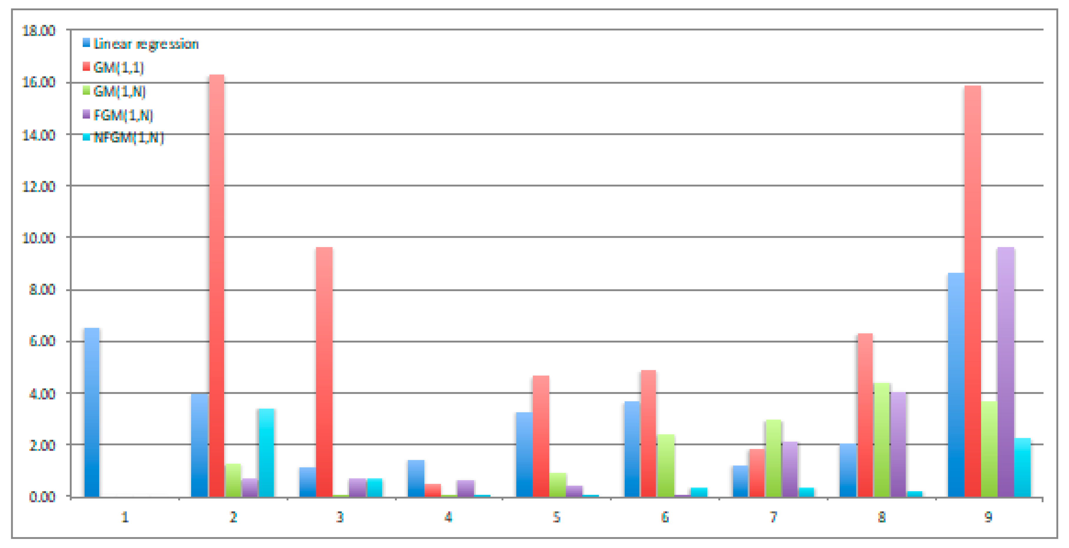
No.	Actual	Linear Regression		GM(1,1)		GM(1,N)		FGM(1,N)		NFGM(1,N)
		Predicted	APE	Predicted	APE	Predicted	APE	Predicted	APE	Predicted	APE
1	11.4918	12.2438	6.54	11.4918	0.00	11.4918	0.00	11.4918	0.00	11.4918	0.00
2	12.2255	12.7083	3.95	10.2363	16.27	12.0729	1.25	12.1431	0.67	11.8068	3.43
3	13.3201	13.4741	1.16	12.041	9.60	13.3124	0.06	13.2250	0.71	13.2241	0.72
4	14.9530	14.7367	1.45	15.0235	0.47	14.9529	0.00	14.8553	0.65	14.9533	0.00
5	17.3891	16.8184	3.28	18.2006	4.67	17.2267	0.93	17.3104	0.45	17.3901	0.01
6	21.0232	20.2505	3.68	22.0495	4.88	20.5136	2.42	21.0355	0.06	20.9479	0.36
7	26.2226	25.9092	1.20	26.7124	1.87	25.4344	3.01	26.7891	2.16	26.3175	0.36
8	34.5325	35.2387	2.05	32.3614	6.29	33.0049	4.42	35.9340	4.06	34.6176	0.25
	MAPE		2.91		5.51		1.51		1.10		0.64
9	46.5982	50.6204	8.63	39.205	15.87	44.8886	3.67	51.0725	9.60	47.6437	2.24

. The MAPEs of the linear regression, GM(1,1), GM(1,N), FGM(1,N), and NFGM(1,N) models in relation to model fitting are 2.91%, 5.51%, 1.51%, 1.10%, and 0.64%, respectively. The MAPEs of the ex-post testing are 8.63%, 15.87%, 3.67%, 9.60%, and 2.24%, respectively. As can be seen from Table 1, the prediction accuracy of the NFGM(1,N) model is much better than that of the other models, whether for model fitting or ex-post testing. Figure 1 shows the superiority of the prediction accuracy of the proposed NFGM(1,N) model over the linear regression model, GM(1,1), GM(1,N), and FGM(1,N) models. Therefore, the proposed NFGM(1,N) model performs well in this numerical example compared with the other models.

4. Empirical Study

4.1. Data Description

Because the prediction accuracy of the proposed NFGM(1,N) model for the numerical example has been proved to be better than that of the other models, it is applied to forecast China’s CO₂e by considering the effect of OFDI. In this study, the NFGM(1,N) model is constructed for the CO₂e as a system characteristic behavior sequence and the OFDI as a relevant variable sequence. More specifically, based on the commitments made by at the UN Climate Change Summit, the CO₂e per unit of GDP in China is chosen to represent the CO₂e, and the total amount of OFDI is selected to represent the OFDI. The raw data, shown in

Table 2. Carbon emissions (CO₂e) and outward foreign direct investment (OFDI) for 2005–2017.

Year	CO2e	OFDI
2005	2.37	13.73
2006	2.17	23.93
2007	1.82	17.15
2008	1.45	56.74
2009	1.40	43.89
2010	1.29	57.95
2011	1.14	48.42
2012	1.03	64.96
2013	0.96	72.97
2014	0.87	123.13
2015	0.83	174.39
2016	0.81	216.42
2017	0.76	138.29

, were obtained from the International Energy Association (https://www.iea.org) and the Development Indicators from the World Bank (https://data.worldbank.org). The data from 2005 to 2014 are reserved for model fitting, and the data from 2015 to 2017 are used for ex-post testing.

4.2. Empirical Results

Following the modeling process mentioned above, the NFGM(1,N) model can be formulated as follows:

$$\frac{d{x}_1^{(0.01)}(t)}{dt}+0.1445x_1^{(0.01)}(t)=0.000104{(x_2^{(0.3)}(t))}^{0.91}+0.0405$$

where the optimal fractional orders for the CO₂e and OFDI, and the optimal value of the power are 0.01, 0.3, and 0.91, respectively. The values of the fractional order indicate that giving greater weight to new information improves prediction accuracy, which is also consistent with the principle of new information priority. As explained by Wu et al. [17] and Ding et al. [4], the driving coefficient b_i can be used to interpret the relationship between the system characteristic behavior and relevant factors. In this study, the driving coefficient is b₂ = 1.04 × 10⁻⁴, which indicates that there is a positive relationship between the CO₂e and OFDI. In other words, the CO₂e increase with increasing OFDI. To examine the prediction accuracy of the proposed NFGM(1,N) model, this model is compared with the ARMA model, linear regression model, GM(1,1), GM(1,N), and FGM(1,N) models. The actual and predicted values of the five competing models are displayed in

Table 3. Prediction accuracies of the competing models for CO₂e.

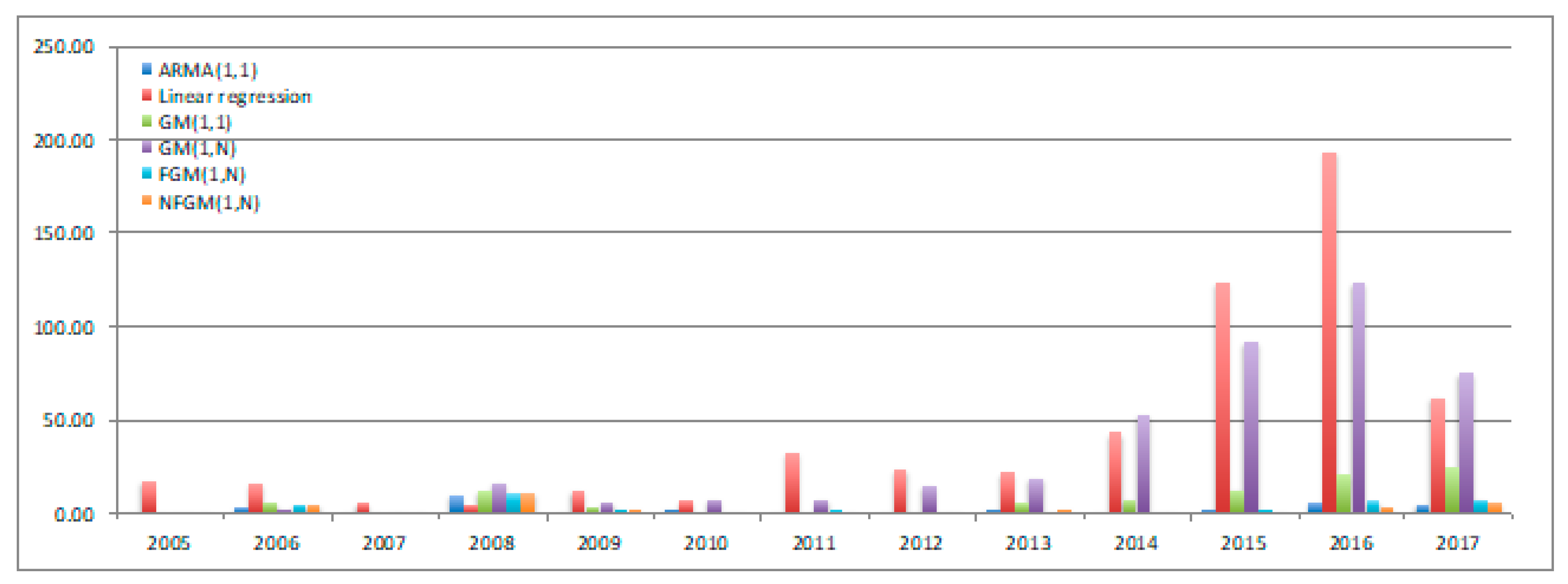
Year	Actual	ARMA(1,1)		Linear Regression		GM(1,1)		GM(1,N)		FGM(1,N)		NFGM(1,N)
		Predicted	APE	Predicted	APE	Predicted	APE	Predicted	APE	Predicted	APE	Predicted	APE
2005	2.37	2.37	0.00	1.97	16.78	2.37	0.00	2.37	0.00	2.37	0.00	2.37	0.00
2006	2.17	2.10	3.13	1.83	15.45	2.04	5.78	2.11	2.50	2.07	4.64	2.07	4.62
2007	1.82	1.82	0.07	1.92	5.46	1.82	0.25	1.82	0.03	1.81	0.48	1.81	0.54
2008	1.45	1.59	9.85	1.39	4.24	1.62	11.63	1.68	16.07	1.61	10.70	1.61	10.74
2009	1.40	1.41	0.70	1.56	11.80	1.44	3.28	1.48	5.96	1.43	2.25	1.43	2.08
2010	1.29	1.25	2.54	1.37	6.76	1.29	0.03	1.38	7.41	1.28	0.58	1.28	0.82
2011	1.14	1.13	0.63	1.50	32.34	1.15	0.99	1.22	7.29	1.15	1.35	1.14	0.71
2012	1.03	1.02	0.93	1.28	23.77	1.02	1.20	1.18	14.44	1.04	0.77	1.03	0.05
2013	0.96	0.94	2.25	1.17	22.01	0.91	5.25	1.14	18.23	0.95	1.19	0.94	2.05
2014	0.87	0.87	0.65	0.50	43.18	0.81	7.27	1.34	52.77	0.87	0.05	0.87	0.03
MAPE			2.08		18.18		3.57		12.47		2.20		2.16
2015	0.83	0.81	1.84	−0.19	123.34	0.72	12.56	1.59	92.07	0.81	1.69	0.82	0.20
2016	0.81	0.76	6.16	−0.76	193.19	0.64	20.90	1.82	123.25	0.76	6.53	0.79	3.41
2017	0.76	0.72	4.94	0.29	61.59	0.57	24.77	1.33	74.94	0.71	7.45	0.72	5.58
MAPE			4.32		126.04		19.41		96.75		5.22		3.06

. Table 3 shows that the MAPEs of the ARMA model, linear regression model, GM(1,1), GM(1,N), FGM(1,N), and NFGM(1,N) models for model fitting are 2.08%, 18.18%, 3.57%, 12.47%, 2.20%, and 2.16%, respectively. The MAPEs in relation to ex-post testing are 4.32%, 126.04%, 19.41%, 96.75%, 5.22%, and 3.06%, respectively. Thus, although the prediction accuracy of the NFGM(1,N) model is slightly inferior to that of the ARMA model for model fitting, the prediction accuracy of NFGM(1,N) is much better than that of the other competing models for ex-post testing.

The prediction precision of different models is illustrated in Figure 2.

The above results confirm that the proposed NFGM(1,N) model has good practicability, and it can better predict China’s CO₂e by considering the effect of OFDI than the other models. Therefore, it has been applied to forecast the CO₂e from 2018 to 2030. The predicted amount of OFDI from 2018 to 2030 is generated by the GM(1,1) model. The predicted value of the relevant factor from 2018 to 2030 is then substituted into the NFGM(1,N) model, which thereby enables China’s CO₂e predictions, after considering the effect of OFDI, to be obtained correspondingly. The predicted OFDI and CO₂e are shown in

Table 4. Predicted OFDI and CO₂e in 2018–2030.

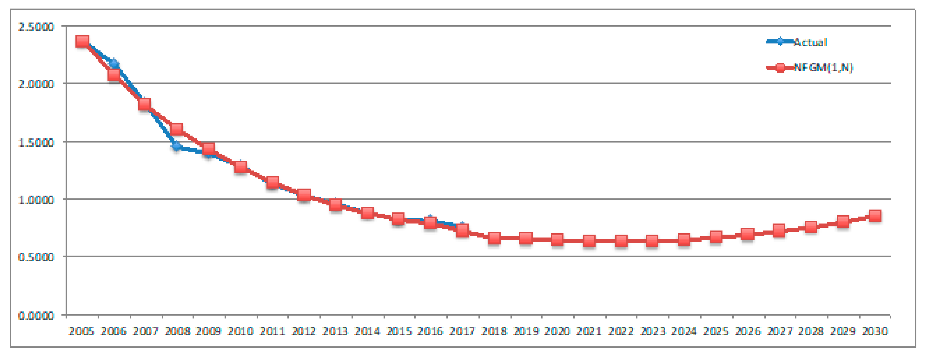
Year	OFDI Prediction	CO2e Prediction
2018	96.47	0.66
2019	203.89	0.66
2020	230.88	0.64
2021	261.44	0.63
2022	296.04	0.63
2023	335.23	0.64
2024	379.60	0.65
2025	429.85	0.67
2026	486.75	0.69
2027	551.18	0.72
2028	624.13	0.76
2029	706.75	0.80
2030	800.30	0.85

. It is noteworthy that China’s carbon emissions will decrease initially, and then climb. Additionally, the prediction of China’s CO₂e in 2020 and 2030 are 0.64 and 0.85, respectively, which represent reductions of 72.83% and 63.97%, respectively, compared with that of 2005. The calculation results show that through unremitting efforts, China can fulfill the CO₂e reduction commitments.

Figure 3 is an intuitive display of the prediction results of CO₂e for the model fitting, ex-post, and out-sample forecasting. From Figure 3 and Table 4, the data sequence of the prediction results indicates that there is a U-shaped relationship between CO₂e and OFDIs.

4.3. Discussion and Suggestions

To determine whether China can deliver on its carbon reduction commitments, this study proposed an NFGM(1,N) model to forecast China’s CO₂e by considering the nonlinear relationship with OFDI. This model was then applied to forecast the CO₂e in China from 2018 to 2030. Several conclusions can be obtained. First, based on the driving coefficient of the NFGM(1,N) model, the increasing OFDI increases the CO₂e in China, which is consistent with the previous studies of Yang and Sun [27] and Liu and Li [13]. As far as this relationship is concerned, the carbon emission transferring effect and technology spillover effect of OFDI are not so clear. The reason for this result may be that, on the one hand, China’s OFDI mainly focuses on low energy consumption industries such as the service industry; thus, industries with high emissions remain in the home country. On the other hand, China’s current OFDI is mainly motivated by resource seeking, rather than technology seeking, so the influence on technological upgrading in the home country is insignificant. Second, the relationship between the CO₂e and OFDI is U-shaped from the perspective view of prediction. According to the forecasts, although China can achieve the emission reduction goal in 2020 and 2030, due to the long-term possibility of emissions increasing, China still faces great pressure to reduce the CO₂e.

Based on the forecast results, China’s CO₂e appear to be on an upward trajectory in the future. In the face of this less-than-optimistic situation, appropriate policies and suggestions are proposed in the study. First, the government should encourage OFDI with technology-seeking motivation. Although rising OFDI could lead to higher carbon emissions in the future, the reverse spillover effect on technological upgrading that has been confirmed by many studies should not be overlooked. Therefore, the government should encourage OFDI with a technology-seeking orientation. In particular, OFDI to the countries with advanced technologies should be encouraged, which can enable domestic enterprises to absorb more advanced knowledge and technology and promote domestic carbon productivity. Second, the government should formulate long-term CO₂e reduction plans. It can be seen from the relationship that the conflict between OFDI and CO₂e cannot be easily resolved in the short term. As an important component of the “opening-up” strategy, in one respect, access to resources, advanced technology, and markets through OFDI can be important drivers of domestic economic development. In another respect, although it promotes economic development, OFDI will cause an increase in carbon emissions. In the long run, the low-carbon economy should be regarded as the strategic goal of any development in China. Although China’s CO₂e reduction commitments can be achieved, formulating appropriate long-term plans for OFDI and CO₂e reduction are still needed to promote sustainable economic development.

5. Conclusions

China, as the largest developing country, has been plagued by the problem of excessive CO₂e for many years. Whether China can fulfill its commitments to emission reduction has become a global focus. Since the Belt and Road Initiative was put forward, OFDI has been increasing, and this has become an important part of the opening-up strategy. Meanwhile, due to the increasing emphasis on environmental protection, the issues related to the impact of OFDI on CO₂e have received general attention. Therefore, this study proposed an NFGM(1,N) model to accurately predict China’s CO₂e by considering the nonlinear effect of OFDI. The results showed that the prediction accuracy of the proposed NFGM(1,N) model was superior to the other competing prediction models.

The NFGM(1,N) model was applied to the prediction of China’s CO₂e for the 2018–2030 period because it has the smallest rate of error. According to the forecasts, China’s CO₂e will decrease by 72.83% and 63.97% in 2020 and 2030, respectively, compared to 2005. Moreover, the prediction of China’s CO₂e presents a U-shaped trend in the long run, which indicates that China still faces numerous pressures related to CO₂e reduction. Therefore, China’s government should encourage OFDI motivated by technology seeking, maximize the reverse spillover effects on home country technologies, and develop long-term plans to further reduce CO₂e and to promote sustainable economic development.

All the empirical results showed that the proposed NFGM(1,N) model had a higher prediction accuracy than the other models and was an appropriate tool to forecast China’s CO₂e. However, based on the empirical results, for the year 2008, the difference between actual value and predicted value in NFGM(1,N) model is much larger than other year. The larger error may be due to the impact on the global economy of the sudden global financial crisis in 2008. Furthermore, COVID-19 swept the world at the end of 2019 and the beginning of 2020, which disastrously impacts the global economy, and more or less affects China’s OFDI and CO₂e in 2020, resulting in a deviation between the predicted value and the real value. The influence of shock disturbances has always been a huge challenge for any prediction model [44]. Therefore, in future studies, the prediction model will be further improved to reduce the influence of shock disturbances, such as global financial crisis and COVID-19, on the predicted results. Additionally, different optimization algorithms, including neural networks, PSO, and others can be introduced into the NFGM(1,N) model to determine the optimal parameters. Furthermore, some approaches, such as the GM(1,1) model, Fourier series, and Markov chain, are available to combine with the NFGM(1,N) as the residual modification model to further improve the prediction accuracy. Finally, the other relevant factors related to CO₂e should be further analyzed.

References

- IEA. World Energy Outlook 2008. Available online: http://www.worldenergyoutlook.org/ (accessed on 6 April 2020).
- Dong, K.Y.; Hochman, G.; Zhang, Y.Q.; Sun, R.J.; Li, H.; Liao, H. CO2 emissions, economic and population growth, and renewable energy: Empirical evidence across regions. Energy Econ. 2018, 75, 180–192. [Google Scholar] [CrossRef]
- Wang, Q.; Jiang, R. Is china’s economic growth decoupled from carbon emissions? J. Clean. Prod. 2019, 225, 1194–1208. [Google Scholar] [CrossRef]
- Ding, S.; Dang, Y.G.; Li, X.M.; Wang, J.J.; Zhao, K. Forecasting chinese CO2 emissions from fuel combustion using a novel grey multivariable model. J. Clean. Prod. 2017, 162, 1527–1538. [Google Scholar] [CrossRef]
- Wu, L.F.; Liu, S.F.; Liu, D.L.; Fang, Z.G.; Xu, H.Y. Modelling and forecasting CO2 emissions in the brics (brazil, russia, india, china, and south africa) countries using a novel multi-variable grey model. Energy 2015, 79, 489–495. [Google Scholar] [CrossRef]
- Wang, S.J.; Shi, C.Y.; Fang, C.L.; Feng, K.S. Examining the spatial variations of determinants of energy-related CO2 emissions in china at the city level using geographically weighted regression model. Appl. Energy 2019, 235, 95–105. [Google Scholar] [CrossRef]
- Mello, D.; Luiz, R. Foreign direct investment in developing countries and growth: A selective survey. J. Dev. Stud. 1997, 34, 1–34. [Google Scholar] [CrossRef]
- Khachoo, Q.; Sharma, R. Fdi and innovation: An investigation into intra- and inter- industry effects. Glob. Econ. Rev. 2016, 45, 311–330. [Google Scholar] [CrossRef]
- Zhu, L.; Jeon, B.N. International r&d spillovers: Trade, fdi, and information technology as spillover channels. Rev. Int. Econ. 2007, 15, 955–976. [Google Scholar]
- Yue, W.; Du, L. The effects of fdi and odi on the development of low carbon economy and the inspiration for b&r strategy. Wuhan Univ. J. Soc. Sci. 2017, 70, 52–60. [Google Scholar]
- Shahbaz, M.; Balsalobre-Lorente, D.; Sinha, A. Foreign direct investment-CO2 emissions nexus in middle east and north african countries: Importance of biomass energy consumption. J. Clean. Prod. 2019, 217, 603–614. [Google Scholar] [CrossRef]
- Kojima, K. Direct Foreign Investment: A Japanese Model of Multinational Business Operation; Crooom Helm: London, UK, 1978. [Google Scholar]
- Liu, H.Y.; Li, M. The home country effect research of china’s ofdi on carbon emissions. J. Ind. Technol. Econ. 2016, 35, 12–18. [Google Scholar]
- Jiang, H.; Kong, P.Y.; Hu, Y.-C.; Jiang, P. Forecasting china’s CO2 emissions by considering interaction of bilateral fdi using the improved grey multivariable verhulst model. Environ. Dev. Sustain. 2020, 1–16. [Google Scholar] [CrossRef]
- Deng, J.L. Introduction to grey system theory. J. Grey Syst. 1989, 1, 1–24. [Google Scholar]
- Zeng, B.; Luo, C.M.; Liu, S.F.; Li, C. A novel multi-variable grey forecasting model and its application in forecasting the amount of motor vehicles in beijing. Comput. Ind. Eng. 2016, 101, 479–489. [Google Scholar] [CrossRef]
- Wu, L.F.; Gao, X.H.; Xiao, Y.L.; Yang, Y.J.; Chen, X.N. Using a novel multi-variable grey model to forecast the electricity consumption of shandong province in china. Energy 2018, 157, 327–335. [Google Scholar] [CrossRef]
- Zeng, B.; Liu, S.; Cuevas, C. A self-adaptive intelligence gray prediction model with the optimal fractional order accumulating operator and its application. Math. Methods Appl. Sci. 2017, 40, 7843–7857. [Google Scholar] [CrossRef]
- Mao, S.H.; Xiao, X.P.; Gao, M.Y.; Wang, X.P.; He, Q. Nonlinear fractional order grey model of urban traffic flow short-term prediction. J. Grey Syst. 2018, 30, 1–17. [Google Scholar]
- Wu, W.Q.; Ma, X.; Zeng, B.; Wang, Y.; Cai, W. Forecasting short-term renewable energy consumption of china using a novel fractional nonlinear grey bernoulli model. Renew. Energy 2019, 140, 70–87. [Google Scholar] [CrossRef]
- Wang, Z.X.; Ye, D.J. Forecasting chinese carbon emissions from fossil energy consumption using non-linear grey multivariable models. J. Clean. Prod. 2017, 142, 600–612. [Google Scholar] [CrossRef]
- Yuan, Y.B.; Zhao, H.; Yuan, X.H.; Chen, L.Y.; Lei, X.H. Application of fractional order-based grey power model in water consumption prediction. Environ. Earth Sci. 2019, 78, 266. [Google Scholar] [CrossRef]
- Wang, Z.X.; Li, Q. Modelling the nonlinear relationship between CO2 emissions and economic growth using a pso algorithm-based grey verhulst model. J. Clean. Prod. 2019, 207, 214–224. [Google Scholar] [CrossRef]
- Nie, F.; Liu, H.Y. Carbon emissions effect of china’s ofdi evidence from urbanization threshold model. China Popul. Resour. Environ. 2016, 26, 123–131. [Google Scholar]
- Liu, H.Y.; Gong, M.Q. A study on the factor market distortion and carbon emission scale effect of two-way fdi. China Population. Resour. Environ. 2018, 28, 27–35. [Google Scholar]
- Long, R.Y.; Zhou, Y. Effect of ofdi reverse technology spillover on regional carbon productivity in China. Ecol. Econ. 2017, 33, 58–62. [Google Scholar]
- Yang, H.; Sun, J. Influence of two-way investment on technological progress and environment: Based on panel threshold model analysis. Sci. Technol. Manag. Res. 2019, 39, 103–109. [Google Scholar]
- Buckley, P.J.; Clegg, L.J.; Cross, A.R.; Liu, X.; Voll, H.; Zheng, P. The determinants of chinese outward foreign direct investment. J. Int. Bus. Stud. 2007, 38, 499–518. [Google Scholar] [CrossRef]
- Fei, N.Y. Low-carbon effects of chinese foreign direct investment. Resour. Dev. Mark. 2014, 30, 984–989. [Google Scholar]
- Luo, L.W.; Cheng, X.J. Path construction of china’s outward foreign direct investment for pushing forward low-carbon economy. Technol. Econ. 2013, 32, 76–82. [Google Scholar]
- Huang, J. Threshold effect of fdi on china’s carbon emission intensity. Stat. Decis. 2017, 33, 108–111. [Google Scholar]
- Zhou, J.Q.; Han, Y.; Zhang, Y. The influence mechanism and effect of foreign investment on china’s carbon emissions. J. Beijing Inst. Technol. Soc. Sci. Ed. 2015, 17, 46–53. [Google Scholar]
- Yu, Y.; Xu, W. Impact of fdi and r&d on china’s industrial CO2 emissions reduction and trend prediction. Atmos. Pollut. Res. 2019, 10, 1627–1635. [Google Scholar]
- Jiang, H.; Hu, Y.-C.; Lin, J.-Y.; Jiang, P. Analyzing china’s ofdi using a novel multivariate grey prediction model with fourier series. Int. J. Intell. Comput. Cybern. 2019, 12, 352–371. [Google Scholar] [CrossRef]
- Wu, W.Z.; Zhang, T. An improved gray interval forecast method and its application. Commun. Stat.-Theory Methods 2019, 49, 1120–1131. [Google Scholar] [CrossRef]
- Li, F.F.; Xu, Z.; Ma, H. Can china achieve its CO2 emissions peak by 2030? Ecol. Indic. 2018, 84, 337–344. [Google Scholar] [CrossRef]
- Meng, M.; Niu, D.; Shang, W. A small-sample hybrid model for forecasting energy-related CO2 emissions. Energy 2014, 64, 673–677. [Google Scholar] [CrossRef]
- Pao, H.-T.; Fu, H.-C.; Tseng, C.-L. Forecasting of CO2 emissions, energy consumption and economic growth in china using an improved grey model. Energy 2012, 40, 400–409. [Google Scholar] [CrossRef]
- Wu, W.Q.; Ma, X.; Zhang, Y.Y.; Li, W.P.; Wang, Y. A novel conformable fractional non-homogeneous grey model for forecasting carbon dioxide emissions of brics countries. Sci. Total Environ. 2020, 707, 135447. [Google Scholar] [CrossRef]
- Ma, X.; Xie, M.; Wu, W.Q.; Zeng, B.; Wang, Y.; Wu, X.X. The novel fractional discrete multivariate grey system model and its applications. Appl. Math. Model. 2019, 70, 402–424. [Google Scholar] [CrossRef]
- Wu, L.F.; Liu, S.F.; Yao, L.G.; Yan, S.L.; Liu, D.L. Grey system model with the fractional order accumulation. Commun. Nonlinear Sci. Numer. Simul. 2013, 18, 1775–1785. [Google Scholar] [CrossRef]
- Wang, Z.X.; Dang, Y.g.; Zhao, J.Y. Optimized gm(1,1) power model and its application. Syst. Eng. Theory Pract. 2012, 34, 1973–1978. [Google Scholar]
- Zeng, L. Analysing the high-tech industry with a multivariable grey forecasting model based on fractional order accumulation. Kybernetes 2019, 48, 1158–1174. [Google Scholar] [CrossRef]
- Liu, S.F.; Lin, Y. Grey Systems: Theory and Applications; Springer: Berlin/Heidelberg, Germany, 2010. [Google Scholar]